13
NONPARAMETRIC STATISTICAL INFERENCE
13.1 INTRODUCTION
In all the problems of statistical inference considered so far, we assumed that the distribution of the random variable being sampled is known except, perhaps, for some parameters. In practice, however, the functional form of the distribution is seldom, if ever, known. It is therefore desirable to devise methods that are free of this assumption concerning distribution. In this chapter we study some procedures that are commonly referred to as distribution-free or nonparametric methods. The term “distribution-free” refers to the fact that no assumptions are made about the underlying distribution except that the distribution function being sampled is absolutely continuous. The term “nonparametric” refers to the fact that there are no parameters involved in the traditional sense of the term “parameter” used thus far. To be sure, there is a parameter which indexes the family of absolutely continuous DFs, but it is not numerical and hence the parameter set cannot be represented as a subset of ![]() n, for any
n, for any ![]() . The restriction to absolutely continuous distribution functions is a simplifying assumption that allows us to use the probability integral transformation (Theorem 5.3.1) and the fact that ties occur with probability 0.
. The restriction to absolutely continuous distribution functions is a simplifying assumption that allows us to use the probability integral transformation (Theorem 5.3.1) and the fact that ties occur with probability 0.
Section 13.2 is devoted to the problem of unbiased (nonparametric) estimation. We develop the theory of U-statistics since many estimators and test statistics may be viewed as U-statistics. Sections 13.3 through 13.5 deal with some common hypotheses testing problems. In Section 13.6 we investigate applications of order statistics in nonparametric methods. Section 13.7 considers underlying assumptions in some common parametric problems and the effect of relaxing these assumptions.
13.2 U-STATISTICS
In Chapter 6 we encountered several nonparametric estimators. For example, the empirical DF defined in Section 6.3 as an estimator of the population DF is distribution-free, and so also are the sample moments as estimators of the population moments. These are examples of what are known as U-statistics which lead to unbiased estimators of population characteristics. In this section we study the general theory of U-statistics. Although the thrust of this investigation is unbiased estimation, many of the U-statistics defined in this section may be used as test statistics.
Let X1,X2,…, Xn be iid RVs with common law ![]() (X), and let
(X), and let ![]() be the class of all possible distributions of X that consists of the absolutely continuous or discrete distributions, or subclasses of these.
be the class of all possible distributions of X that consists of the absolutely continuous or discrete distributions, or subclasses of these.
We have already encountered many examples of complete statistics or complete families of distributions in Chapter 8.
The following result is stated without proof. For the proof we refer to Fraser [32, pp. 27–30, 139–142].
Clearly, the U-statistic defined in (3) is symmetric in the Xi’s, and
Moreover, U(X) is a function of the complete sufficient statistic X(1), X(2),…,X(n). It follows from Theorem 8.4.6 that it is UMVUE of its expected value.
For estimating μ3(F), a symmetric kernel is ![]() so that the corresponding U-statistic is
so that the corresponding U-statistic is

For estimating F(x) a symmetric kernel is ![]() so the corresponding U-statistic is
so the corresponding U-statistic is

and for estimating ![]() the U-statistic is
the U-statistic is

Finally, for estimatin ![]() the U-statistic is
the U-statistic is

Now note that the numerator has ![]() factors involving n, while the denominator has m such factors so that for
factors involving n, while the denominator has m such factors so that for ![]() , the ratio involving n goes to 0 as
, the ratio involving n goes to 0 as ![]() . For
. For ![]() , this ratio
, this ratio ![]() and
and

as ![]()
Finally we state, without proof, the following result due to Hoeffding [45], which establishes the asymptotic normality of a suitably centered and normed U-statistic. For proof we refer to Lehmann [61, pp. 364–365] or Randles and Wolfe [85, p. 82].
The concept of U-statistics can be extended to multiple random samples. We will restrict ourselves to the case of two samples. Let ![]() and
and ![]() be two independent random samples from DFs F and G, respectively.
be two independent random samples from DFs F and G, respectively.
The statistic T in Definition 8 is called a kernel of g and a symmetrized version of T, Ts is called a symmetric kernel of g. Without loss of generality therefore we assume that the two-sample kernel T in (9) is a symmetric kernel.
Finally we state, without proof, the two-sample analog of Theorem 3 which establishes the asymptotic normality of the two-sample U-statistic defined in (10).
PROBLEMS 13.2
- Let
 be a probability space, and let
  . Let A be a Borel subset of
  , and consider the parameter
  . Is d estimable? If so, what is the degree? Find the UMVUE for d, based on a sample of size n, assuming that
  is the class of all continuous distributions.
 - Let X1, X2,…, Xm and Y1, Y2,…, Yn be independent random samples from two absolutely continuous DFs. Find the UMVUEs of (a) E{XY} and (b)
 .
. - Let (X1, Y1), (X2, Y2),…,(Xn, Yn) be a random sample from an absolutely continuous distribution. Find the UMVUEs of (a) E(XY) and (b)
 .
. - Let T(X1, X2,…, Xn) be a statistic that is symmetric in the observations. Show that T can be written as a function of the order statistic. Conversely, if T (X1, X2,…,Xn) can be written as a function of the order statistic, T is symmetric in the observations.
- Let X1, X2, …,Xn be a random sample from an absolutely continuous
 . Find U-statistics for
  . Find the corresponding expressions for the variance of the U-statistic in each case.
 - In Example 3, show that μ2(F) is not estimable with one observation. That is, show that the degree of μ2(F) where
 , the class of all distributions with finite second moment, is 2.
 - Show that for
 .
. - Let X1, X2, …,Xn be a random sample from an absolutely continuous . Let

Find the U-statistic estimator of g(F) and its variance.
13.3 SOME SINGLE-SAMPLE PROBLEMS
Let X1, X2,…,Xn be a random sample from a DF F. In Section 13.2 we studied properties of U-statistics as nonparametric estimators of parameters g(F). In this section we consider some nonparametric tests of hypotheses. Often the test statistic may be viewed as a function of a U-statistic.
13.3.1 Goodness-of-Fit Problem
The problem of fit is to test the hypothesis that the sample comes from a specified DF F0 against the alternative that it is from some other DF F, where ![]() for some
for some ![]() . In Section 10.3 we studied the chi-square test of goodness of fit for testing
. In Section 10.3 we studied the chi-square test of goodness of fit for testing ![]() . Here we consider the Kolmogorov–Smirnov test of H0. Since H0 concerns the underlying DF of the X’s, it is natural to compare the U-statistic estimator of
. Here we consider the Kolmogorov–Smirnov test of H0. Since H0 concerns the underlying DF of the X’s, it is natural to compare the U-statistic estimator of ![]() with the specified DF F0 under H0. The U-statistic for
with the specified DF F0 under H0. The U-statistic for ![]() is the empirical
is the empirical ![]() .
.
Since F(X(i)) is the ith-order statistic of a sample from U (0,1) irrespective of what F is, as long as it is continuous, we see that the distribution of ![]() is independent of F. Similarly,
is independent of F. Similarly,

and the result follows.
Without loss of generality, therefore, we assume that F is the DF of a U(0,1) RV.
We will not prove this result here. Let Dn, α be the upper α-percent point of the distribution of Dn, that is, ![]() . The exact distribution of Dn for selected values of n and α has been tabulated by Miller [74], Owen [79], and Birnbaum [9]. The large-sample distribution of Dn was derived by Kolmogorov [53], and we state it without proof.
. The exact distribution of Dn for selected values of n and α has been tabulated by Miller [74], Owen [79], and Birnbaum [9]. The large-sample distribution of Dn was derived by Kolmogorov [53], and we state it without proof.
The statistics ![]() and
and ![]() have the same distribution because of symmetry, and their common distribution is given by the following theorem.
have the same distribution because of symmetry, and their common distribution is given by the following theorem.
Tables for the critical values ![]() where
where ![]() , are also available for selected values of n and α; see Birnbaum and Tingey [8]. Table ST7 at the end of this book gives
, are also available for selected values of n and α; see Birnbaum and Tingey [8]. Table ST7 at the end of this book gives ![]() and Dn, α for some selected values of n and α. For large samples Smirnov [108] showed that
and Dn, α for some selected values of n and α. For large samples Smirnov [108] showed that
In fact, in view of (9), the statistic ![]() has a limiting χ2(2) distribution, for
has a limiting χ2(2) distribution, for ![]() if and only if
if and only if ![]() , and the result follows since
, and the result follows since
so that
which is the DF of a χ2 (2) RV.
It is worthwhile to compare the chi-square test of goodness of fit and the Kolmogorov–Smirnov test. The latter treats individual observations directly, whereas the former discretizes the data and sometimes loses information through grouping. Moreover, the Kolmogorov–Smirnov test is applicable even in the case of very small samples, but the chi-square test is essentially for large samples.
The chi-square test can be applied when the data are discrete or continuous, but the Kolmogorov–Smirnov test assumes continuity of the DF. This means that the latter test provides a more refined analysis of the data. If the distribution is actually discontinuous, the Kolmogorov–Smirnov test is conservative in that it favors H0.
We next turn our attention to some other uses of the Kolmogorov–Smirnov statistic. Let X1, X2,…,Xn be a sample from a DF F, and let ![]() be the sample DF. The estimate
be the sample DF. The estimate ![]() of F for large n should be close to F. Indeed,
of F for large n should be close to F. Indeed,

and, since ![]() , we have
, we have

Thus ![]() can be made close to F with high probability by choosing λ and large enough n. The Kolmogorov–Smirnov statistic enables us to determine the smallest n such that the error in estimation never exceeds a fixed value ε with a large probability 1 – α. Since
can be made close to F with high probability by choosing λ and large enough n. The Kolmogorov–Smirnov statistic enables us to determine the smallest n such that the error in estimation never exceeds a fixed value ε with a large probability 1 – α. Since
![]() ; and, given ε and α, we can read n from the tables. For large n, we can use the asymptotic distribution of Dn and solve
; and, given ε and α, we can read n from the tables. For large n, we can use the asymptotic distribution of Dn and solve ![]() for n.
for n.
We can also form confidence bounds for F. Given α and n, we first find Dn,α such that
which is the same as

Thus
Define
And
Then the region between Ln(x) and Un(x) can be used as a confidence band for F(x) with associated confidence coefficient 1 – α.
13.3.2 Problem of Location
Let X1,X2,…,Xn be a sample of size n from some unknown DF F. Let p be a positive real number, ![]() , and let
, and let ![]() P (F) denote the quantile of order p for the DF F. In the following analysis we assume that F is absolutely continuous. The problem of location is to test
P (F) denote the quantile of order p for the DF F. In the following analysis we assume that F is absolutely continuous. The problem of location is to test ![]() a given number, against one of the alternatives
a given number, against one of the alternatives ![]() and
and ![]() . The problem of location and symmetry is to test
. The problem of location and symmetry is to test ![]() , and F is symmetric against
, and F is symmetric against ![]() or F is not symmetric.
or F is not symmetric.
We consider two tests of location. First, we describe the sign test.
13.3.2.1 The Sign Test
Let X1,X2,…,Xn be iid RVs with common PDF f. Consider the hypothesis testing problem
where ![]() P(f) is the quantile of order p of PDF f,
P(f) is the quantile of order p of PDF f, ![]() . Let
. Let ![]() . Then the corresponding U-statistic is given by
. Then the corresponding U-statistic is given by
the number of positive elements in X1 – ![]() 0, X2 –
0, X2 – ![]() 0,…,Xn –
0,…,Xn – ![]() 0. Clearly, P(Xi =
0. Clearly, P(Xi = ![]() 0) = 0. Fraser [32, pp. 167–170] has shown that a UMP test of H0 against H1 is given by
0) = 0. Fraser [32, pp. 167–170] has shown that a UMP test of H0 against H1 is given by

where c and γ are chosen from the size restriction

Note that, under ![]() , so that
, so that ![]() and
and ![]() . The same test is UMP for
. The same test is UMP for ![]() against
against ![]() . For the two-sided case, Fraser [32, p. 171] shows that the two-sided sign test is UMP unbiased.
. For the two-sided case, Fraser [32, p. 171] shows that the two-sided sign test is UMP unbiased.
If, in particular, ![]() is the median of f, then
is the median of f, then ![]() under H0. In this case one can also use the sign test to test
under H0. In this case one can also use the sign test to test ![]() , F is symmetric.
, F is symmetric.
For large n one can use the normal approximation to binomial to find c and γ in (19).
We have to find c and γ such that

From the table of cumulative binomial distribution (Table ST1) for ![]() ,
, ![]() , we see that
, we see that ![]() . Then γ is given by
. Then γ is given by

Thus
In our case the number of positive signs, xi – 195, i = 1,2,..., 12, is 7, so we reject H0 that the upper quartile is ≤195.
The single-sample sign test described above can easily be modified to apply to sampling from a bivariate population. Let (X1, Y1), (X2, Y2),…,(Xn, Yn) be a random sample from a bivariate population. Let ![]() , and assume that Zi has an absolutely continuous DF. Then one can test hypotheses concerning the order parameters of Z by using the sign test. A hypothesis of interest here is that Z has a given median
, and assume that Zi has an absolutely continuous DF. Then one can test hypotheses concerning the order parameters of Z by using the sign test. A hypothesis of interest here is that Z has a given median ![]() 0. Without loss of generality let
0. Without loss of generality let ![]() . Then
. Then ![]() , that is,
, that is, ![]() . Note that med(Z) is not necessarily equal to med(X) – med(Y), so that H0 is not that
. Note that med(Z) is not necessarily equal to med(X) – med(Y), so that H0 is not that ![]() but that
but that ![]() . The sign test is UMP against one-sided alternatives and UMP unbiased against two-sided alternatives.
. The sign test is UMP against one-sided alternatives and UMP unbiased against two-sided alternatives.
Using the two-sided sign test, we cannot reject H0 at level α = 0.05, since ![]() . The RVs Zi can be considered to be distributed normally, so that under H0 the common mean of Zi,'s is 0. Using a paired comparison t-test on the data, we can show that
. The RVs Zi can be considered to be distributed normally, so that under H0 the common mean of Zi,'s is 0. Using a paired comparison t-test on the data, we can show that ![]() for 9 d.f., so we cannot reject the hypothesis of equality of means of X and Y at level
for 9 d.f., so we cannot reject the hypothesis of equality of means of X and Y at level ![]() .
.
Finally, we consider the Wilcoxon signed-ranks test.
13.3.2.2 The Wilcoxon Signed-Ranks Test
The sign test for median and symmetry loses information since it ignores the magnitude of the difference between the observations and the hypothesized median. The Wilcoxon signed-ranks test provides an alternative test of location (and symmetry) that also takes into account the magnitudes of these differences.
Let X1, X2,…, Xn be iid RVs with common absolutely continuous DF F, which is symmetric about the median ![]() 1/2. The problem is to test
1/2. The problem is to test ![]() against the usual one- or two-sided alternatives. Without loss of generality, we assume that
against the usual one- or two-sided alternatives. Without loss of generality, we assume that ![]() . Then
. Then ![]() for all
for all ![]() . To test
. To test ![]() or
or ![]() , we first arrange |X1|, |X2|,…,|Xn| in increasing order of magnitude, and assign ranks 1, 2,…,n, keeping track of the original signs of Xi. For example, if
, we first arrange |X1|, |X2|,…,|Xn| in increasing order of magnitude, and assign ranks 1, 2,…,n, keeping track of the original signs of Xi. For example, if ![]() and
and ![]() , the rank of |X1| is 3, of |X2| is 1, of |X3| is 4, and of |X4| is 2.
, the rank of |X1| is 3, of |X2| is 1, of |X3| is 4, and of |X4| is 2.
Let

Then, under H0, we expect T+ and T- to be the same. Note that
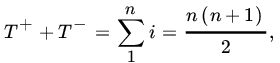
so that T+ and T-are linearly related and offer equivalent criteria. Let us define
and write ![]() for the rank of |Xi| Then
for the rank of |Xi| Then ![]() and
and ![]() . Also,
. Also,

The statistic T+ (or T-) is known as the Wilcoxon statistic. A large value of T+ (or, equivalently, a small value of T−) means that most of the large deviations from 0 are positive, and therefore we reject H0 in favor of the alternative, ![]() .
.
A similar analysis applies to the other two alternatives. We record the results as follows:
| Test | ||
| H0 | H1 | Reject H0 if |
We now show how the Wilcoxon signed-ranks test statistic is related to the U-statistic estimate of ![]() . Recall from Example 13.2.6 that the corresponding U-statistic is
. Recall from Example 13.2.6 that the corresponding U-statistic is

First note that

Next note that for ![]() if and only if
if and only if ![]() and |X(i) | |X(j) | . It follows that
and |X(i) | |X(j) | . It follows that ![]() is the signed-rank of X(j). Consequently,
is the signed-rank of X(j). Consequently,

where U1 is the U-statistic for ![]() .
.
We next compute the distribution of T+ for small samples. The distribution of T+ is tabulated by Kraft and Van Eeden [55, pp. 221–223].
Let

Note that ![]() if all differences have negative signs, and
if all differences have negative signs, and ![]() if all differences have positive signs. Here a difference means a difference between the observations and the postulated value of the median. T+ is completely determined by the indicators Z(i), so that the sample space can be considered as a set of 2n n-tuples (z1, z2,…, zn), where each zi is 0 or 1. Under
if all differences have positive signs. Here a difference means a difference between the observations and the postulated value of the median. T+ is completely determined by the indicators Z(i), so that the sample space can be considered as a set of 2n n-tuples (z1, z2,…, zn), where each zi is 0 or 1. Under ![]() and each arrangement is equally likely. Thus
and each arrangement is equally likely. Thus

Note that every assignment has a conjugate assignment with plus and minus signs interchanged so that for this conjugate, T+ is given by

Thus under H0 the distribution of T+ is symmetric about the mean ![]() .
.
Remark 2. If we have n independent pairs of observations (X1,Y1),(X2,Y2),,…,(Xn,Yn) from a bivariate DF, we form the differences ![]() ,
, ![]() . Assuming that Z1, Z2,…,Zn are (independent) observations from a population of differences with absolutely continuous DF F that is symmetric with median
. Assuming that Z1, Z2,…,Zn are (independent) observations from a population of differences with absolutely continuous DF F that is symmetric with median ![]() 1/2, we can use the Wilcoxon statistic to test
1/2, we can use the Wilcoxon statistic to test ![]() .
.
We present some examples.
From Table ST10, we reject H0 at ![]() if either T+ > 46 or T+ < 9. Since T+ > 9 and < 46, we accept H0. Note that hypothesis H0 was also accepted by the sign test.
if either T+ > 46 or T+ < 9. Since T+ > 9 and < 46, we accept H0. Note that hypothesis H0 was also accepted by the sign test.
For large samples we use the normal approximation. In fact, from (26) we see that
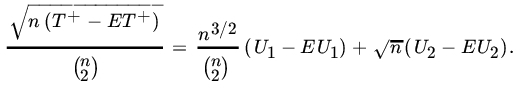
Clearly, ![]() and since
and since ![]() , the first term →0 in probability as
, the first term →0 in probability as ![]() . By Slutsky’s theorem (Theorem 7.2.15) it follows that
. By Slutsky’s theorem (Theorem 7.2.15) it follows that

have the same limiting distribution. From Theorem 13.2.3 and Example 13.2.7 it follows that ![]() , and hence
, and hence ![]() , has a limiting normal distribution with mean 0 and variance
, has a limiting normal distribution with mean 0 and variance
Under H0, the RVs iZ(i) are independent b(1,1/2) so

Also, under H0, F is continuous and symmetric so

and

Thus ![]() so that
so that

However,
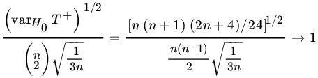
as n→∞. Consequently, under H0

Thus, for large enough n we can determine the critical values for a test based on T+ by using normal approximation.
As an example, take ![]() . From Table ST10 the P-value associated with
. From Table ST10 the P-value associated with ![]() is 0.10. Using normal approximation
is 0.10. Using normal approximation

PROBLEMS 13.3
- Prove Theorem 4.
- A random sample of size 16 from a continuous DF on [0,1] yields the following data: 0.59,0.72,0.47,0.43,0.31,0.56,0.22,0.90,0.96,0.78,0.66,0.18,0.73,0.43,0.58,0.11. Test the hypothesis that the sample comes from U[0,1].
- Test the goodness of fit of normality for the data of Problem 10.3.6, using the Kolmogorov–Smirnov test.
Do not reject H0.
- For the data of Problem 10.3.6 find a 0.95 level confidence band for the distribution function.
- The following data represent a sample of size 20 from U[0,1]: 0.277,0.435,0.130, 0.143, 0.853, 0.889, 0.294, 0.697, 0.940, 0.648, 0.324, 0.482, 0.540, 0.152, 0.477, 0.667, 0.741, 0.882, 0.885, 0.740. Construct a .90 level confidence band for F(x).
- In Problem 5 test the hypothesis that the distribution is U[0,1]. Take
 .
. - For the data of Example 2 test, by means of the sign test, the null hypothesis
 against
  .
.
Reject H0.
- For the data of Problem 5 test the hypothesis that the quantile of order
 is 0.20.
 - For the data of Problem 10.4.8 use the sign test to test the hypothesis of no difference between the two averages.
- Use the sign test for the data of Problem 10.4.9 to test the hypothesis of no difference in grade-point averages.
Do not reject H0 at 0.05 level.
- For the data of Problem 5 apply the signed-rank test to test
 against
 , do not reject H0.
 - For the data of Problems 10.4.8 and 10.4.9 apply the signed-rank test to the differences to test
 against
  .
.
(Second part)
 , do not reject H0 at
  .
.
13.4 SOME TWO-SAMPLE PROBLEMS
In this section we consider some two-sample tests. Let X1,X2,…,Xm and Y1,Y2 ,…,Yn be independent samples from two absolutely continuous distribution functions FX and FY, respectively. The problem is to test the null hypothesis ![]() for all
for all ![]() against the usual one- and two-sided alternatives.
against the usual one- and two-sided alternatives.
Tests of H0 depend on the type of alternative specified. We state some of the alternatives of interest even though we will not consider all of these in this text.
- Location alternative:
 ,
, 
- Scale alternative:
 ,
, 
- Lehmann alternative:
 ,
,  .
. - Stochastic alternative:
 for all x, and
  for at least one x.
 - General alternative:
 for some x.
Some comments are in order. Clearly I through IV are special cases of V. Alternatives I and II show differences in FX and FY in location and scale, respectively. Alternative III states that ![]() . In the special case when θ is an integer it states that Y has the same distribution as the smallest of the
. In the special case when θ is an integer it states that Y has the same distribution as the smallest of the ![]() of X-variables. A similar alternative to test that is sometimes used is
of X-variables. A similar alternative to test that is sometimes used is ![]() for some
for some ![]() and all x. When α is an integer, this states that Y is distributed as the largest of the α X-variables. Alternative IV refers to the relative magnitudes of X’s and Y’s. It states that
and all x. When α is an integer, this states that Y is distributed as the largest of the α X-variables. Alternative IV refers to the relative magnitudes of X’s and Y’s. It states that
so that
for all x. In other words, X’s tend to be larger than the Y’s.
A similar interpretation may be given to the one-sided alternative ![]() . In the special case where both X and Y are normal RVs with means μ1, μ2 and common variance σ2
. In the special case where both X and Y are normal RVs with means μ1, μ2 and common variance σ2 ![]() corresponds to and
corresponds to and ![]() and
and ![]() corresponds to
corresponds to ![]()
In this section we consider some common two-sample tests for location (Case I) and stochastic ordering (Case IV) alternatives. First, note that a test of stochastic ordering may also be used as a test of less restrictive location alternatives since, for example, ![]() corresponds to larger Y’s and hence larger location for Y. Second, we note that the chi-square test of homogeneity described in Section 10.3 can be used to test general alternatives (Case V)
corresponds to larger Y’s and hence larger location for Y. Second, we note that the chi-square test of homogeneity described in Section 10.3 can be used to test general alternatives (Case V) ![]() for some x. Briefly, one partitions the real line into Borel sets A1,A2,…,Ak. Let
for some x. Briefly, one partitions the real line into Borel sets A1,A2,…,Ak. Let
![]() . Under
. Under ![]() ,
, ![]() ,
, ![]() , which is the problem of testing equality of two independent multinomial distributions discussed in Section 10.3.
, which is the problem of testing equality of two independent multinomial distributions discussed in Section 10.3.
We first consider a simple test of location. This test, based on the sample median of the combined sample, is a test of the equality of medians of the two DFs. It will tend to accept ![]() even if the shapes of F and G are different as long as their medians are equal.
even if the shapes of F and G are different as long as their medians are equal.
13.4.1 Median Test
The combined sample X1,X2,…,Xm, Y1,Y2,…,Yn is ordered and a sample median is found. If ![]() is odd, the median is the
is odd, the median is the ![]() th value in the ordered arrangement. If
th value in the ordered arrangement. If ![]() is even, the median is any number between the two middle values. Let V be the number of observed values of X that are less than or equal to the sample median for the combined sample. If V is large, it is reasonable to conclude that the actual median of X is smaller than the median of Y. One therefore rejects
is even, the median is any number between the two middle values. Let V be the number of observed values of X that are less than or equal to the sample median for the combined sample. If V is large, it is reasonable to conclude that the actual median of X is smaller than the median of Y. One therefore rejects ![]() in favor of
in favor of ![]() for all x and
for all x and ![]() for some x if V is too large, that is, if
for some x if V is too large, that is, if ![]() . If, however, the alternative is
. If, however, the alternative is ![]() for all x and
for all x and ![]() for some x, the median test rejects H0 if
for some x, the median test rejects H0 if ![]() .
.
For the two-sided alternative that ![]() for some x, we use the two-sided test.
for some x, we use the two-sided test.
We next compute the null distribution of the RV V. If ![]() , p a positive integer, then
, p a positive integer, then

Here ![]() . If
. If ![]() , is an integer, the
, is an integer, the ![]() th value is the median in the combined sample, and
th value is the median in the combined sample, and

Remark 1. Under H0 we expect ![]() observations above the median and
observations above the median and ![]() below the median. One can therefore apply the chi-square test with 1 d.f. to test H0 against the two-sided alternative.
below the median. One can therefore apply the chi-square test with 1 d.f. to test H0 against the two-sided alternative.
We now consider two tests of the stochastic alternatives. As mentioned earlier they may also be used as tests of location.
13.4.2 Kolmogorov–Smirnov Test
Let X1,X2 ,…,Xm and Y1,Y2,…,Yn be independent random samples from continuous DFs F and G, respectively. Let ![]() and
and ![]() , respectively, be the empirical DFs of the X’s and the Y’s. Recall the
, respectively, be the empirical DFs of the X’s and the Y’s. Recall the ![]() is the U-statistic for F and
is the U-statistic for F and ![]() , that for G. Under
, that for G. Under ![]() for all x, we expect a reasonable agreement between the two sample DFs. We define
for all x, we expect a reasonable agreement between the two sample DFs. We define
Then Dm, n may be used to test H0 against the two-sided alternative ![]() for some x. The test rejects H0 at level α if
for some x. The test rejects H0 at level α if
where ![]() .
.
Similarly, one can define the one-sided statistics
and
to be used against the one-sided alternatives

and

respectively.
For small samples tables due to Massey [72] are available. In Table ST9, we give the values of Dm,n,α and ![]() for some selected values of m, n, and α. Table ST8 gives the corresponding values for the
for some selected values of m, n, and α. Table ST8 gives the corresponding values for the ![]() case.
case.
For large samples we use the limiting result due to Smirnov [107]. Let ![]() .
.
Then


Relations (10) and (11) give the distribution of ![]() and Dm,n, respectively, under
and Dm,n, respectively, under ![]() for all
for all ![]() .
.
Let us first apply the Kolmogorov–Smirnov test to test H0 that the population distribution of length of life for the two brands is the same.
| x | |||
| 30 | 0 | ||
| 40 | |||
| 45 | |||
| 50 | |||
| 55 | 1 | ||
| 60 | 1 | 1 | 0 |
From Table ST8, the critical value for ![]() at level
at level ![]() is
is ![]() . Since
. Since ![]() , we accept H0 that the population distribution for the length of life for the two brands is the same.
, we accept H0 that the population distribution for the length of life for the two brands is the same.
Let us next apply the two-sample t-test. We have ![]() ,
, ![]() ,
, ![]() ,
, ![]() ,
, ![]() . Thus
. Thus
Since ![]() , we accept the hypothesis that the two samples come from the same (normal) population.
, we accept the hypothesis that the two samples come from the same (normal) population.
The second test of stochastic ordering alternatives we consider is the Mann–Whitney–Wilcoxon test which can be viewed as a test based on a U-statistic.
13.4.3 The Mann–Whitney–Wilcoxon Test
Let X1,X2,…,Xm and Y1,Y2,…,Yn be independent samples from two continuous DFs, F and G, respectively. As in Example 13.2.10, let

for ![]() ,
, ![]() . Recall that T(Xi ; Yj) is an unbiased estimator of
. Recall that T(Xi ; Yj) is an unbiased estimator of ![]() and the two sample U-statistic for g is given by
and the two sample U-statistic for g is given by ![]() . For notational convenience, let us write
. For notational convenience, let us write

Then U is the number of values of X1,X2,…,Xm that are smaller than each of Y1,Y2,…,Yn. The statistic U is called the Mann–Whitney statistic. An alternative equivalent form using Wilcoxon scores is the linear rank statistic given by

where Qj = rank of Yj among the combined ![]() observations. Indeed,
observations. Indeed,
Thus

so that U and W are equivalent test statistics. Hence the name Mann–Whitney–Wilcoxon Test. We will restrict attention to U as the test statistic.
Note that ![]() if all the Xi,’s are larger than all the Yj’s and
if all the Xi,’s are larger than all the Yj’s and ![]() if all the Xi’s are smaller than all the Yj’s, because then there are m
if all the Xi’s are smaller than all the Yj’s, because then there are m ![]() ,
, ![]() , and so on. Thus
, and so on. Thus ![]() . If U is large, the values of Y tend to be larger than the values of X (Y is stochastically larger than X), and this supports the alternative
. If U is large, the values of Y tend to be larger than the values of X (Y is stochastically larger than X), and this supports the alternative ![]() for all x and
for all x and ![]() for some x. Similarly, if U is small, the Y values tend to be smaller than the X values, and this supports the alternative
for some x. Similarly, if U is small, the Y values tend to be smaller than the X values, and this supports the alternative ![]() for all x and F(x)
for all x and F(x) ![]() G(x) for some x. We summarize these results as follows:
G(x) for some x. We summarize these results as follows:
| H0 | H1 | Reject H0 if |
To compute the critical values we need the null distribution of U. Let
We will set up a difference equation relating pm, n to pm–1,n and pm, n–1. If the observations are arranged in increasing order of magnitude, the largest value can be either an x value or a y value. Under H0, all ![]() values are equally likely, so the probability that the largest value will be an x value is
values are equally likely, so the probability that the largest value will be an x value is ![]() and that it will be a y value is
and that it will be a y value is ![]() .
.
Now, if the largest value is an x, it does not contribute to U, and the remaining ![]() values of x and n values of y can be arranged to give the observed value
values of x and n values of y can be arranged to give the observed value ![]() with probability pm–1,n(u). If the largest value is a Y, this value is larger than all the m x’s. Thus, to get
with probability pm–1,n(u). If the largest value is a Y, this value is larger than all the m x’s. Thus, to get ![]() , the remaining
, the remaining ![]() values of Y and m values of x contribute
values of Y and m values of x contribute ![]() . It follows that
. It follows that
If ![]() , then for
, then for ![]()
If ![]() ,
, ![]() , then
, then
and
For small values of m and n one can easily compute the null PMF of U. Thus, if ![]() , then
, then
If ![]() ,
, ![]() , then
, then
Tables for critical values are available for small values of m and n, ![]() . See, for example, Auble [3] or Mann and Whitney [71]. Table ST11 gives the values of uα for which
. See, for example, Auble [3] or Mann and Whitney [71]. Table ST11 gives the values of uα for which ![]() for some selected values of m, n, and α.
for some selected values of m, n, and α.
If m, n are large we can use the asymptotic normality of U. In Example 13.2.11 we showed that, under H0,
as ![]() such that
such that ![]() constant. The approximation is fairly good for
constant. The approximation is fairly good for ![]() .
.
PROBLEMS 13.4
- For the data of Example 4 apply the median test.
- Twelve 4-year-old boys and twelve 4-year-old girls were observed during two 15-minute play sessions, and each child’s play during these two periods was scored as follows for incidence and degree of aggression:
- Boys: 86, 69,72, 65, 113, 65, 118, 45, 141, 104, 41, 50
- Girls: 55, 40, 22, 58, 16, 7, 9, 16, 26, 36, 20, 15
Test the hypothesis that there were sex differences in the amount of aggression shown, using (a) the median test and (b) the Mann-Whitney-Wilcoxon test (Siegel [105]).
- To compare the variability of two brands of tires, the following mileages (1000 miles) were obtained for eight tires of each kind:
- Brand A:32.1, 20.6, 17.8, 28.4, 19.6, 21.4, 19.9, 30.1
- Brand B:19.8, 27.6, 30.8, 27.6, 34.1, 18.7, 16.9, 17.9
Test the null hypothesis that the two samples come from the same population, using the Mann–Whitney–Wilcoxon test.
- Use the data of Problem 2 to apply the Kolmogorov−Smirnov test.
- Apply the Kolmogorov−Smirnov test to the data of Problem 3.
- Yet another test for testing
 against general alternatives is the so-called runs test. A run is a succession of one or more identical symbols which are preceded and followed by a different symbol (or no symbol). The length of a run is the number of like symbols in a run. The total number of runs, R, in the combined sample of X’s and Y’s when arranged in increasing order can be used as a test of H0. Under H0 the X and Y symbols are expected to be well-mixed. A small value of R supports
  . A test based on R is appropriate only for two-sided (general) alternatives. Tables of critical values are available. For large samples, one uses normal approximation:
  .
.
- Let
 of X-runs,
  -runs, and
  . Under H0, show that

Where
 if
if  if
if  ,
,  and
and  .
. - Show that

- Let
- Fifteen 3-year-old boys and 15 3-year-old girls were observed during two sessions of recess in a nursery school. Each child’s play was scored for incidence and degree of aggression as follows:
- Boys: 96 65 74 78 82 121 68 79 111 48 53 92 81 31 40
- Girls: 12 47 32 59 83 14 32 15 17 82 21 34 9 15 51
Is there evidence to suggest that there are sex differences in the incidence and amount of aggression? Use both Mann–Whitney–Wilcoxon and runs tests.
13.5 TESTS OF INDEPENDENCE
Let X and Y be two RVs with joint DF F(x, y), and let F1 and F2, respectively, be the marginal DFs of X and Y. In this section we study some tests of the hypothesis of independence, namely,
against the alternative
If the joint distribution function F is bivariate normal, we know that X and Y are independent if and only if the correlation coefficient ![]() . In this case, the test of independence is to test
. In this case, the test of independence is to test ![]() .
.
In the nonparametric situation the most commonly used test of independence is the chi-square test, which we now study.
13.5.1 Chi-square Test of Independence—Contingency Tables
Let X and Y be two RVs, and suppose that we have n observations on (X,Y). Let us divide the space of values assumed by X (the real line) into r mutually exclusive intervals A1, A2,…,Ar. Similarly, the space of values of Y is divided into c disjoint intervals B1, B2,…,Bc. As a rule of thumb, we choose the length of each interval in such a way that the probability that X(Y) lies in an interval is approximately (1/r)(1/c). Moreover, it is desirable to have n/r and n/c at least equal to 5. Let Xij denote the number of pairs (Xk, Yk), ![]() , that lie in Ai × Bj, and let
, that lie in Ai × Bj, and let
Where ![]() ,
, ![]() . If each pij is known, the quantity
. If each pij is known, the quantity

has approximately a chi-square distribution with ![]() d.f., provided that n is large (see Theorem 10.3.2.). If X and Y are independent,
d.f., provided that n is large (see Theorem 10.3.2.). If X and Y are independent, ![]() . Let us write
. Let us write ![]() and
and ![]() . Then under
. Then under ![]() ,
, ![]() ,
, ![]() . In practice, pij will not be known. We replace pij by their estimates. Under H0, we estimate pi· by
. In practice, pij will not be known. We replace pij by their estimates. Under H0, we estimate pi· by

and p·j by

Since ![]() we have estimated only
we have estimated only ![]() parameters. It follows (see Theorem 10.3.4) that the RV
parameters. It follows (see Theorem 10.3.4) that the RV

is asymptotically distributed as χ2 with ![]() d.f., under H0. The null hypothesis is rejected if the computed value of U exceeds χ 2(r-1)(c-1),α..
d.f., under H0. The null hypothesis is rejected if the computed value of U exceeds χ 2(r-1)(c-1),α..
It is frequently convenient to list the observed and expected frequencies of the rc events Ai × Bj in an r × c table, called a contingency table, as follows:
| Observed Frequencies, Oij | Expected Frequencies, Eij | ||||||
| B1 | B2…Bc | B1 | B2…Bc | ||||
| A1 | X11 | X12…X2c | A1 | np1.p.1 | np1.p.2… np1.p.c | np1 | |
| A2 | X21 | X22…X2c | A2 | np2.p.1 | np2.p.2… np2.p.c | np2 | |
| . | . | .... | . | . | . | . …. | |
| . | . | .... | . | . | . | . …. | |
| . | . | .... | . | . | . | . …. | |
| Ar | Xr1 | Xr2…Xrc | Ar | npr.p.1 | npr.p.c… npr.p.c | npr | |
| n | np.1 | np.2 np.c | n | ||||
Note that the Xij’s in the table are frequencies. Once the category Ai × Bj is determined for an observation (X, Y), numerical values of X and Y are irrelevant. Next, we need to compute the expected frequency table. This is done quite simply by multiplying the row and column totals for each pair (i, j) and dividing the product by n. Then we compute the quantity

and compare it with the tabulated ![]() value. In this form the test can be applied even to qualitative data. A1, A2, …,Ar and B1, B2,…,Bc represent the two attributes, and the null hypothesis to be tested is that the attributes A and B are independent.
value. In this form the test can be applied even to qualitative data. A1, A2, …,Ar and B1, B2,…,Bc represent the two attributes, and the null hypothesis to be tested is that the attributes A and B are independent.
13.5.2 Kendall’s Tau
Let (X1, Y1), (X2, Y2),…,(Xn, Yn) be a sample from a bivariate population.
Writing πc and πd for the probability of perfect concordance and of perfect discordance, respectively, we have
and
and, if the marginal distributions of X and Y are continuous,

If the marginal distributions of X and Y are continuous, we may rewrite (11), in view of (10), as follows:
In particular, if X and Y are independent and continuous RVs, then
since then ![]() is a symmetric RV. Then
is a symmetric RV. Then

and it follows that ![]() for independent continuous RVs.
for independent continuous RVs.
Note that, in general, ![]() does not imply independence. However, for the bivariate normal distribution
does not imply independence. However, for the bivariate normal distribution ![]() if and only if the correlation coefficient ρ, between X and Y, is 0, so that
if and only if the correlation coefficient ρ, between X and Y, is 0, so that ![]() if and only if X and Y are independent (Problem 6).
if and only if X and Y are independent (Problem 6).
Let
Then ![]() , and we see that
, and we see that ![]() is estimable of degree 2, with symmetric kernel ψ defined in (13). The corresponding one-sample U-statistic is given by
is estimable of degree 2, with symmetric kernel ψ defined in (13). The corresponding one-sample U-statistic is given by
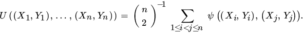
Then the corresponding estimator of Kendall’s tau is
and is called Kendall’s sample correlation coefficient.
Note that ![]() . To test H0 that X and Y are independent against H1 : X and Y are dependent, we reject H0 if |T| is large. Under H0,
. To test H0 that X and Y are independent against H1 : X and Y are dependent, we reject H0 if |T| is large. Under H0, ![]() , so that the null distribution of T is symmetric about 0. Thus we reject H0 at level α if the observed value of T, t, satisfies |t|
, so that the null distribution of T is symmetric about 0. Thus we reject H0 at level α if the observed value of T, t, satisfies |t| ![]() tα/2, where
tα/2, where ![]() .
.
For small values of n the null distribution can be directly evaluated. Values for ![]() are tabulated by Kendall [51]. Table ST12 gives the values of Sα for which
are tabulated by Kendall [51]. Table ST12 gives the values of Sα for which ![]() , where
, where ![]() T for selected values of n and α.
T for selected values of n and α.
For a direct evaluation of the null distribution we note that the numerical value of T is clearly invariant under all order-preserving transformations. It is therefore convenient to order X and Y values and assign them ranks. If we write the pairs from the smallest to the largest according to, say, X values, then the number of pairs of values of ![]() for which
for which ![]() is the number of concordant pairs, P.
is the number of concordant pairs, P.
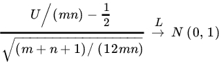
For large n we can use an extension of Theorem 13.3.3 to bivariate case to conclude that ![]() , where
, where
Under H0, it can be shown that

See, for example, Kendall [51], Randles and Wolfe [85], or Gibbons [35]. Approximation is good for ![]() .
.
13.5.3 Spearman’s Rank Correlation Coefficient
Let (X1, Y1), (X2, Y2),…, (Xn,Yn) be a sample from a bivariate population. In Section 6.3 we defined the sample correlation coefficient by

where

If the sample values X1,X2,…,Xn and Y1,Y2,…,Yn are each ranked from 1 to n in increasing order of magnitude separately, and if the X’s and Y’s have continuous DFs, we get a unique set of rankings. The data will then reduce to n pairs of rankings. Let us write
then Ri and Si ∈ {1,2,…,n}. Also


and
Substituting in (16), we obtain

Writing ![]() , we have
, we have

and it follows that

The statistic R defined in (20) and (21) is called Spearman’s rank correlation coefficient (see also Example 4.5.2).
From (20) we see that

Under H0, the RVs X and Y are independent, so that the ranks Ri and Si are also independent. It follows that

and

Thus we should reject H0 if the absolute value of R is large, that is, reject H0 if
where ![]() . To compute Rα we need the null distribution of R. For this purpose it is convenient to assume, without loss of generality, that
. To compute Rα we need the null distribution of R. For this purpose it is convenient to assume, without loss of generality, that ![]() . Then
. Then ![]() ,
, ![]() . Under H0, X and Y being independent, the n! pairs (i,Si) of ranks are equally likely. It follows that
. Under H0, X and Y being independent, the n! pairs (i,Si) of ranks are equally likely. It follows that

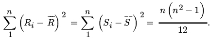
Note that ![]() , and the extreme values can occur only when either the rankings match, that is,
, and the extreme values can occur only when either the rankings match, that is, ![]() , in which case
, in which case ![]() , or
, or ![]() , in which case
, in which case ![]() . Moreover, one need compute only one half of the distribution, since it is symmetric about 0 (Problem 7).
. Moreover, one need compute only one half of the distribution, since it is symmetric about 0 (Problem 7).
In the following example we will compute the distribution of R for ![]() and 4. The exact
and 4. The exact ![]() complete distribution of
complete distribution of ![]() , and hence R, for
, and hence R, for ![]() has been tabulated by Kendall [51]. Table ST13 gives the values of Rα for some selected values of n and α.
has been tabulated by Kendall [51]. Table ST13 gives the values of Rα for some selected values of n and α.
Since ![]() , we cannot reject H0 at
, we cannot reject H0 at ![]() or
or ![]() .
.
For large samples it is possible to use a normal approximation. It can be shown (see, e.g., Fraser [32, pp. 247–248]) that under H0 the RV

or, equivalently,
has approximately a standard normal distribution. The approximation is good for ![]() .
.
PROBLEMS 13.5
- A sample of 240 men was classified according to characteristics A and B. Characteristic A was subdivided into four classes A1, A2, A3, and A4, while B was subdivided into three classes B1, B2, and B3, with the following result:
A1 A2 A3 A4 B1 12 25 32 11 80 B2 17 18 22 23 80 B3 21 17 16 26 80 50 60 70 60 240 Is there evidence to support the theory that A and B are independent?
- The following data represent the blood types and ethnic groups of a sample of Iraqi citizens:
Blood Type Ethnic Group O A B AB Kurd 531 450 293 226 Arab 174 150 133 36 Jew 42 26 26 8 Turkoman 47 49 22 10 Ossetian 50 59 26 15 Is there evidence to conclude that blood type is independent of ethnic group?
- In a public opinion poll, a random sample of 500 American adults across the country was asked the following question: “Do you believe that there was a concerted effort to cover up the Watergate scandal? Answer yes, no, or no opinion.” The responses according to political beliefs were as follows:
Political Affiliation Response Yes No No Opinion Republican 45 75 30 150 Independent 85 45 20 150 Democrat 140 30 30 200 270 150 80 500 Test the hypothesis that attitude toward the Watergate cover-up is independent of political party affiliation.
- A random sample of 100 families in Bowling Green, Ohio, showed the following distribution of home ownership by family income:
Residential Status Annual Income (dollars) Less than 30,000 30,000-50,000 50,000or Above Home Owner 10 15 30 Renter 8 17 20 Is home ownership in Bowling Green independent of family income?
- In a flower show the judges agreed that five exhibits were outstanding, and these were numbered arbitrarily from 1 to 5. Three judges each arranged these five exhibits in order of merit, giving the following rankings:
Judge A: 5 3 1 2 4 Judge B: 3 1 5 4 2 Judge C: 5 2 3 1 4 Compute the average values of Spearman’s rank correlation coefficient R and Kendall’s sample tau coefficient T from the three possible pairs of rankings.
- For the bivariate normally distributed RV (X, Y) show that
 if and only if X and Y are independent. [Hint: Show that
  , where p is the correlation coefficient between X and Y.]
 - Show that the distribution of Spearman's rank correlation coefficient R is symmetric about 0 under H0.
- In Problem 5 test the null hypothesis that rankings of judge A and judge C are independent. Use both Kendall’s tau and Spearman's rank correlation tests.
- A random sample of 12 couples showed the following distribution of heights:
Couple Height (in.) Couple Height (in.) Husband Wife Husband Wife 1 80 72 7 74 68 2 70 60 8 71 71 3 73 76 9 63 61 4 72 62 10 64 65 5 62 63 11 68 66 6 65 46 12 67 67 - Compute T.
- Compute R.
- Test the hypothesis that the heights of husband and wife are independent, using T as well as R. In each case use the normal approximation.
 ;
; ;
;- Reject H0 in each case.
13.6 SOME APPLICATIONS OF ORDER STATISTICS
In this section we consider some applications of order statistics. We are mainly interested in three applications, namely, tolerance intervals for distributions, coverages, and confidence interval estimates for quantiles and location parameters.
Let X1, X2,…,Xn be a sample of size n from F, and let X(1), X(2), …,X(n) be the corresponding set of order statistics. If the end points of the tolerance interval are two-order statistics X(r), X(s), r ![]() s, we have
s, we have
Since F is continuous, F(X) is U(0, 1), and we have

where U(r), U(s) are the order statistics from U(0,1). Thus (1) reduces to
The statistic ![]() ,
, ![]() , is called the coverage of the interval (X(r),X(s)). More precisely, the differences
, is called the coverage of the interval (X(r),X(s)). More precisely, the differences ![]() , for
, for ![]() , where
, where ![]() and
and ![]() , are called elementary coverages.
, are called elementary coverages.
Since the joint PDF of U(1), U(2),…, U(n) is given by

the joint PDFofV1, V2,…,Vn is easily seen to be

Note that h is symmetric in its arguments. Consequently, Vi’s are exchangeable RVs and the distribution of every sum of r, r ![]() n, of these coverages is the same and, in particular, it is the distribution of
n, of these coverages is the same and, in particular, it is the distribution of ![]() namely,
namely,

The common distribution of elementary coverages is
Thus ![]() and
and ![]() . This may be interpreted as follows: The order statistics X(1),X(2),…,X(n) partition the area under the PDF in
. This may be interpreted as follows: The order statistics X(1),X(2),…,X(n) partition the area under the PDF in ![]() parts such that each part has the same average (expected) area.
parts such that each part has the same average (expected) area.
The sum of any r successive elementary coverages Vi+1,Vi+1 ,…,Vi+r is called an r-coverage. Clearly

and, in particular,) ![]() . Since V's are exchangeable it follows that
. Since V's are exchangeable it follows that
with PDF
From (3), therefore

where the last equality follows from (5.3.48). Given n, p, γ it may not always be possible to find s - r to satisfy (8).
In general, given p, 0 < p < 1, it is possible to choose a sufficiently large sample of size n and a corresponding value of ![]() such that with probability ≥ γ an interval of the form (X(r),X(s)) covers at least 100p percent of the distribution. If
such that with probability ≥ γ an interval of the form (X(r),X(s)) covers at least 100p percent of the distribution. If ![]() is specified as a function of n, one chooses the smallest sample size n.
is specified as a function of n, one chooses the smallest sample size n.
We next consider the use of order statistics in constructing confidence intervals for population quantiles. Let X be an RV with a continuous DF F,0 < p < 1. Then the quantile of order p satisfies
Let X1, X2,…,Xn be n independent observations on X. Then the number of Xi's < ![]() p is an RV that has a binomial distribution with parameters n and p. Similarly, the number of Xi's that are at least
p is an RV that has a binomial distribution with parameters n and p. Similarly, the number of Xi's that are at least ![]() p has a binomial distribution with parameters n and
p has a binomial distribution with parameters n and ![]() .
.
Let X(1),X(2),…,X(n) be the set of order statistics for the sample. Then

Similarly

It follows from (10) and (11) that

It is easy to determine a confidence interval for ![]() p from (12), once the confidence level is given. In practice, one determines r and s such that
p from (12), once the confidence level is given. In practice, one determines r and s such that ![]() is as small as possible, subject to the condition that the level is
is as small as possible, subject to the condition that the level is ![]() .
.
Finally we consider applications of order statistics to constructing confidence intervals for a location parameter. For this purpose we will use the method of test inversion discussed in Chapter 11. We first consider confidence estimation based on the sign test of location.
Let X1,X2,…,Xn be a random sample from a symmetric, continuous ![]() and suppose we wish to find a confidence interval for 6. Let
and suppose we wish to find a confidence interval for 6. Let ![]() of
of ![]() , be the sign-test statistic for testing
, be the sign-test statistic for testing ![]() against
against ![]() . Clearly,
. Clearly, ![]() under H0. The sign-test rejects H0 if
under H0. The sign-test rejects H0 if
for some integer c to be determined from the level of the test. Let ![]() . Then any value of θ is acceptable provided it is greater than the rth smallest observation and smaller than the rth largest observation, giving as confidence interval
. Then any value of θ is acceptable provided it is greater than the rth smallest observation and smaller than the rth largest observation, giving as confidence interval
If we want level ![]() to be associated with (14), we choose c so that the level of test (13) is α.
to be associated with (14), we choose c so that the level of test (13) is α.
We next consider the Wilcoxon signed-ranks test of ![]() to construct a confidence interval for θ. The test statistic in this case is T+ = sum of ranks of positive
to construct a confidence interval for θ. The test statistic in this case is T+ = sum of ranks of positive ![]() 's in the ordered |Xt — θ+|'s. From (13.3.4)
's in the ordered |Xt — θ+|'s. From (13.3.4)

Let ![]() ,
,![]() and order the
and order the  Tij's in increasing order of magnitude
Then using the argument that converts (13) to (14) we see that a confidence interval for θ is given by
Critical values c are taken from Table ST10.
- Find the smallest values of n such that the intervals (a) (X(1),X(n)) and (b) (X(2),X(n-1)) contain the median with probability
 0.90.
0.90.
- 5;
- 8.
- Find the smallest sample size required such that (X(1), X(n)) covers at least 90 percent of the distribution with probability > 0.98.
- Find the relation between n andp such that (X(1),X(n)) covers at least 100p percent of the distribution with probability.
 .
.
 .
. - Given γ, δ, p0, p1 with
 , find the smallest n such that
and

Find also
 .
.[Hint: Use the normal approximation to the binomial distribution.]
 .
. - In Problem 4 find the smallest n and the associated value of
 if
if  ,
,  ,
,  ,
,  .
. - Let X1 , X2,… , X7 be a random sample from a continuous DF F. Compute:
 .
.
 ..
..
- Let X1,X2,…,Xn be iid with common continuous DF F.
- What is the distribution of

for
 ?
? - What is the distribution of
 .
.
- What is the distribution of
13.7 ROBUSTNESS
Most of the statistical inference problems treated in this book are parametric in nature. We have assumed that the functional form of the distribution being sampled is known except for a finite number of parameters. It is to be expected that any estimator or test of hypothesis concerning the unknown parameter constructed on this assumption will perform better than the corresponding nonparametric procedure, provided that the underlying assumptions are satisfied. It is therefore of interest to know how well the parametric optimal tests or estimators constructed for one population perform when the basic assumptions are modified. If we can construct tests or estimators that perform well for a variety of distributions, for example, there would be little point in using the corresponding nonparametric method unless the assumptions are seriously violated.
In practice, one makes many assumptions in parametric inference, and any one or all of these may be violated. Thus one seldom has accurate knowledge about the true underlying distribution. Similarly, the assumption of mutual independence or even identical distribution may not hold. Any test or estimator that performs well under modifications of underlying assumptions is usually referred to as robust.
In this section we will first consider the effect that slight variation in model assumptions have on some common parametric estimators and tests of hypotheses. Next we will consider some corresponding nonparametric competitors and show that they are quite robust.
13.7.1 Effect of Deviations from Model Assumptions on Some Parametric Procedures
Let us first consider the effect of contamination on sample mean as an estimator of the population mean.
The most commonly used estimator of the population mean μ is the sample mean ![]() . It has the property of unbiasedness for all populations with finite mean. For many parent populations (normal, Poisson, Bernoulli, gamma, etc.) it is a complete sufficient statistic and hence a UMVUE. Moreover, it is consistent and has asymptotic normal distribution whenever the conditions of the central limit theorem are satisfied. Nevertheless, the sample mean is affected by extreme observations, and a single observation that is either too large or too small may make
. It has the property of unbiasedness for all populations with finite mean. For many parent populations (normal, Poisson, Bernoulli, gamma, etc.) it is a complete sufficient statistic and hence a UMVUE. Moreover, it is consistent and has asymptotic normal distribution whenever the conditions of the central limit theorem are satisfied. Nevertheless, the sample mean is affected by extreme observations, and a single observation that is either too large or too small may make ![]() worthless as an estimator of μ. Suppose, for example, that X1, X2,…,Xn is a sample from some normal population. Occasionally something happens to the system, and a wild observation is obtained that is, suppose one is sampling from
worthless as an estimator of μ. Suppose, for example, that X1, X2,…,Xn is a sample from some normal population. Occasionally something happens to the system, and a wild observation is obtained that is, suppose one is sampling from ![]() (μ, σ2), say, 100α percent of the time and from
(μ, σ2), say, 100α percent of the time and from ![]() (μ, kσ2), where
(μ, kσ2), where ![]() percent of the time. Here both μ and σ2 are unknown, and one wishes to estimate μ. In this case one is really sampling from the density function
percent of the time. Here both μ and σ2 are unknown, and one wishes to estimate μ. In this case one is really sampling from the density function
Where f0 is the PDF of ![]() (μ, σ2), and f1, the PDF of
(μ, σ2), and f1, the PDF of ![]() (μ, kσ2). Clearly,
(μ, kσ2). Clearly,

is still unbiased for μ. If α is nearly 1, there is no problem since the underlying distribution is nearly (μ, σ2), and ![]() is nearly the UMVUE of μ with variance σ2/n. If
is nearly the UMVUE of μ with variance σ2/n. If ![]() is large (that is, not nearly 0), then, since one is sampling from f, the variance of X1 is σ2 with probability α and is kα 2 with probability
is large (that is, not nearly 0), then, since one is sampling from f, the variance of X1 is σ2 with probability α and is kα 2 with probability ![]() , and we have
, and we have

If ![]() is large,
is large, ![]() is large and we see that even an occasional wild observation makes
is large and we see that even an occasional wild observation makes ![]() subject to a sizable error. The presence of an occasional observation from
subject to a sizable error. The presence of an occasional observation from ![]() (μ, kσ2) is frequently referred to as contamination. The problem is that we do not know, in practice, the distribution of the wild observations and hence we do not know the PDF f. It is known that the sample median is a much better estimator than the mean in the presence of extreme values. In the contamination model discussed above, if we use Z1/2, the sample median of the Xi’s, as an estimator of μ (which is the population median), then for large n
(μ, kσ2) is frequently referred to as contamination. The problem is that we do not know, in practice, the distribution of the wild observations and hence we do not know the PDF f. It is known that the sample median is a much better estimator than the mean in the presence of extreme values. In the contamination model discussed above, if we use Z1/2, the sample median of the Xi’s, as an estimator of μ (which is the population median), then for large n

(See Theorem 7.5.2 and Remark 7.5.7.) Since

we have

As ![]() . If there is no contamination,
. If there is no contamination, ![]() and
and ![]() . Also,
. Also,

which will be close to 1 if α is close to 1. Thus the estimator Z1/2 will not be greatly affected by how large k is, that is, how wild the observations are. We have

Indeed, ![]() as
as ![]() , whereas
, whereas ![]() as
as ![]() . One can check that, when
. One can check that, when ![]() and
and ![]() , the two variances are (approximately) equal. As k becomes larger than 9 or α smaller than 0.915, Z1/2 becomes a better estimator of μ than
, the two variances are (approximately) equal. As k becomes larger than 9 or α smaller than 0.915, Z1/2 becomes a better estimator of μ than ![]() .
.
There are other flaws as well. Suppose, for example, that X1, X2,…,Xn is a sample from ![]() . Then both
. Then both ![]() and
and ![]() , where
, where ![]() , are unbiased for
, are unbiased for ![]() . Also,
. Also, ![]() , and one can show that
, and one can show that ![]() . It follows that the efficiency of
. It follows that the efficiency of ![]() relative to that of T is
relative to that of T is

In fact, ![]() as
as ![]() , so that in sampling from a uniform parent
, so that in sampling from a uniform parent ![]() is much worse than T, even for moderately large values of n.
is much worse than T, even for moderately large values of n.
Let us next turn our attention to the estimation of standard deviation. Let X1, X2, …,Xn be a sample from ![]() (μ, σ2). Then the MLE of σ is
(μ, σ2). Then the MLE of σ is

Note that the lower bound for the variance of any unbiased estimator for σ is σ2/2n. Although ![]() is not unbiased, the estimator
is not unbiased, the estimator
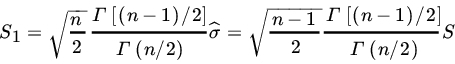
is unbiased for σ Also,

Thus the efficiency of S1 (relative to the estimator with least variance = σ2/2n)is

and →1 as n → ∞. For small n, the efficiency of S1 is considerably smaller than 1. Thus, for ![]() ,
, ![]() and, for
and, for ![]() ,
, ![]() .
.
Yet another estimator of σ is the sample mean deviation
Note that
and

If n is large enough so that ![]() , we see that
, we see that ![]() is nearly unbiased for σ with variance
is nearly unbiased for σ with variance ![]() . The efficiency of S3 is
. The efficiency of S3 is

For large n, the efficiency of S1 relative to S3 is

Now suppose that there is some contamination. As before, let us suppose that for a proportion α of the time we sample from ![]() (μ, σ2) and for a proportion
(μ, σ2) and for a proportion ![]() of the time we get a wild observation from
of the time we get a wild observation from ![]() (μ, kσ2),
(μ, kσ2), ![]() . Assuming that both μ and σ2 are unknown, suppose that we wish to estimateσ. In the notation used above, let
. Assuming that both μ and σ2 are unknown, suppose that we wish to estimateσ. In the notation used above, let
Where f0 is the PDF of ![]() (μ, σ2),and f1, the PDF of us see how even small contamination can make the ma(μ, kσ2). Let us see how even small contamination can make the maximum likelihood estimate
(μ, σ2),and f1, the PDF of us see how even small contamination can make the ma(μ, kσ2). Let us see how even small contamination can make the maximum likelihood estimate ![]() of σ quite useless.
of σ quite useless.
If ![]() is the MLE of θ, and ϕ is a function of θ, then
is the MLE of θ, and ϕ is a function of θ, then ![]() is the MLE of ϕ(θ). Inview of (7.5.7) we get
is the MLE of ϕ(θ). Inview of (7.5.7) we get

Using Theorem 7.3.5, we see that

(drooping the other two terms with n2 and n3 in the denominator), so that
For the density f, we see that
and
It follows that

If we are interested in the effect of very small contamination, ![]() and
and ![]() . Assuming that
. Assuming that ![]() , we see that
, we see that

In the normal case, ![]() and
and ![]() , so that from (11)
, so that from (11)

Thus we see that the mean square error due to a small contamination is now multiplied by a factor ![]() . If, for example,
. If, for example, ![]() , then
, then ![]() . If
. If ![]() , then
, then ![]() , and so on.
, and so on.
A quick comparison with S3 shows that, although S1 (or even ![]() a) is a better estimator of σ than S3 if there is no contamination, S3 becomes a much better estimator in the presence of contamination as k becomes large.
a) is a better estimator of σ than S3 if there is no contamination, S3 becomes a much better estimator in the presence of contamination as k becomes large.
Next we consider the effect of deviation from model assumptions on tests of hypotheses. One of the most commonly used tests in statistics is Student’s t-test for testing the mean of a normal population when the variance is unknown. Let X1, X2,…,Xn be a sample from some population with mean μ and finite variance σ2. As usual, let ![]() denote the sample mean, and S2, the sample variance. If the population being sampled is normal, the t-test rejects
denote the sample mean, and S2, the sample variance. If the population being sampled is normal, the t-test rejects ![]() against
against ![]() at level α if
at level α if ![]() . If n is large, we replace
. If n is large, we replace ![]() by the corresponding critical value, zα/2 under the standard normal law. If the sample does not come from a normal population, the statistic
by the corresponding critical value, zα/2 under the standard normal law. If the sample does not come from a normal population, the statistic ![]() is no longer distributed as a t
is no longer distributed as a t ![]() statistic. If, however, n is sufficiently large, we know that T has an asymptotic normal distribution irrespective of the population being sampled, as long as it has a finite variance. Thus, for large n, the distribution of T is independent of the form of the population, and the t-test is stable. The same considerations apply to testing the difference between two means when the two variances are equal. Although we assumed that n is sufficiently large for Slutsky s result (Theorem 7.2.15) to hold, empirical investigations have shown that the test based on Student s statistic is robust. Thus a significant value of t may not be interpreted to mean a departure from normality of the observations. Let us next consider the effect of departure from independence on the t-distribution. Suppose that the observations X1, X2,…,Xn have a multivariate normal distribution with
statistic. If, however, n is sufficiently large, we know that T has an asymptotic normal distribution irrespective of the population being sampled, as long as it has a finite variance. Thus, for large n, the distribution of T is independent of the form of the population, and the t-test is stable. The same considerations apply to testing the difference between two means when the two variances are equal. Although we assumed that n is sufficiently large for Slutsky s result (Theorem 7.2.15) to hold, empirical investigations have shown that the test based on Student s statistic is robust. Thus a significant value of t may not be interpreted to mean a departure from normality of the observations. Let us next consider the effect of departure from independence on the t-distribution. Suppose that the observations X1, X2,…,Xn have a multivariate normal distribution with ![]() , and ρ as the common correlation coefficient between any Xi and Xj,
, and ρ as the common correlation coefficient between any Xi and Xj, ![]() . Then
. Then

and since Xi’s are exchangeable it follows from Remark 6.3.1 that
For large n, the statistic ![]() will be asymptotically distributed as
will be asymptotically distributed as ![]() , instead of
, instead of ![]() (0, 1). Under H0,
(0, 1). Under H0, ![]() and
and  is distributed as
 ![]() . Consider the ratio
. Consider the ratio

The ratio equals 1 if ![]() but is > 0 for
but is > 0 for ![]() and →∞ as ρ→1. It follows that a large value of T is likely to occur when
and →∞ as ρ→1. It follows that a large value of T is likely to occur when ![]() and is large, even though μ0 is the true value of the mean. Thus a significant value of t may be due to departure from independence, and the effect can be serious.
and is large, even though μ0 is the true value of the mean. Thus a significant value of t may be due to departure from independence, and the effect can be serious.
Next, consider a test of the null hypothesis ![]() against
against ![]() . Under the usual normality assumptions on the observations X1, X2,…Xn, the test statistic used is
. Under the usual normality assumptions on the observations X1, X2,…Xn, the test statistic used is

Which has a ![]() distribution under H0. The usual test is to reject H0 of
distribution under H0. The usual test is to reject H0 of
Let us suppose that X1, X2,…Xn are not normal. It follows from Corollary 2 of Theorem 7.3.4 that

so that

Writing ![]() , we have
, we have

When the Xi’s are not normal, and

when the Xi’s are normal ![]() . Now
. Now ![]() is the sum of n identically distributed but dependent
is the sum of n identically distributed but dependent ![]() , j = 1, 2,…,n. Using a version of the central limit theorem for dependent RVs (see, e.g., Cramér [17, p. 365]), it follows that
, j = 1, 2,…,n. Using a version of the central limit theorem for dependent RVs (see, e.g., Cramér [17, p. 365]), it follows that

under H0, is asymptotically ![]() , and not
, and not ![]() (0, 1)as under the normal theory. As a result the size of the test based on the statistic V0 will be different from the stated level of significance if γ2 differs greatly from 0. It is clear that the effect of violation of the normality assumption can be quite serious on inferences about variances, and the chi-square test is not robust.
(0, 1)as under the normal theory. As a result the size of the test based on the statistic V0 will be different from the stated level of significance if γ2 differs greatly from 0. It is clear that the effect of violation of the normality assumption can be quite serious on inferences about variances, and the chi-square test is not robust.
In the above discussion we have used somewhat crude calculations to investigate the behavior of the most commonly used estimators and test statistics when one or more of the underlying assumptions are violated. Our purpose here was to indicate that some tests or estimators are robust whereas others are not. The moral is clear: One should check carefully to see that the underlying assumptions are satisfied before using parametric procedures.
13.7.2 Some Robust Procedures
Let X1, X2,…, Xn be a random sample from a continuous PDF ![]() and assume that f is symmetric about θ. We shall be interested in estimation or tests of hypotheses concerning θ. Our objective is to find procedures that perform well for several different types of distributions but do not have to be optimal for any particular distribution. We will call such procedures robust. We first consider estimation of θ.
and assume that f is symmetric about θ. We shall be interested in estimation or tests of hypotheses concerning θ. Our objective is to find procedures that perform well for several different types of distributions but do not have to be optimal for any particular distribution. We will call such procedures robust. We first consider estimation of θ.
The estimators fall under one of the following three types:
- Estimators that are functions of
 , where Rj is the rank of Xj, are known as R-estimators. Hodges and Lehmann [44] devised a method of deriving such estimators from rank tests. These include the sample median
  (based on the sign test) and
  based on the Wilcoxon signed-rank test.
 - Estimators of the form
 are called L-estimators, being linear combinations of order statistics. This class includes the median, the mean, and the trimmed mean obtained by dropping a prespecified proportion of extreme observations.
 - Maximum likelihood type estimators obtained as solutions to certain equations
 are called M-estimators. The function
  gives MLEs.
Two extreme examples of trimmed means are the sample mean ![]() and the median
and the median ![]() when all except the central (n odd) or the two central (n even) observations are excluded.
when all except the central (n odd) or the two central (n even) observations are excluded.
We will limit this discussion to four estimators of location, namely, the sample median, trimmed mean, sample mean, and Hodges–Lehmann type estimator based on Wilcoxon signed-rank test. In order to compare the performance of two procedures A and B we will use a (large sample) measure of relative efficiency due to Pitman. Pitman’s asymptotic relative efficiency (ARE) of procedure B relative to procedure A is the limit of the ratio of sample sizes nA/nB, where nA, nB are sample sizes needed for procedures A and B to perform equivalently with respect to a specified criterion. For example, suppose {Tn(B)} and {Tn(A)} are two sequences of estimators for ψ(θ) such that

and

Suppose further that A and B perform equivalently if their asymptotic variances are the same, that is,

Then

Clearly, different performance measures may lead to different measures of ARE.
Similarly if procedures A and B lead to two sequences of tests, then ARE is the limiting ratio of the sample sizes needed by the tests to reach a certain power β0 against the same alternative and at the same limiting level α.
Accordingly, let e(B,A) denote the ARE of B relative to A. If ![]() say, then procedure A requires (approximately) half as many observations as procedure B. We will write eF(B, A), whenever necessary to indicate the dependence of ARE on the underlying DF F.
say, then procedure A requires (approximately) half as many observations as procedure B. We will write eF(B, A), whenever necessary to indicate the dependence of ARE on the underlying DF F.
For detailed discussion of Pitman efficiency we refer to Lehmann ![]() , Lehmann [63, section 5.2], Serfling [102, chapter 10], Randles and Wolfe [85, chapter 5], and Zacks [121]. The expressions for AREs of median and the Hodges-Lehmann estimators of location parameter θ with respect to the sample mean
, Lehmann [63, section 5.2], Serfling [102, chapter 10], Randles and Wolfe [85, chapter 5], and Zacks [121]. The expressions for AREs of median and the Hodges-Lehmann estimators of location parameter θ with respect to the sample mean ![]() are
are

where f is the PDF corresponding to F. In order to get ![]() we use the fact that
we use the fact that

Bickel [5] showed that

where

and ![]() α is the unique αth percentile of F. It is clear from (32) that no closed form expression for
α is the unique αth percentile of F. It is clear from (32) that no closed form expression for ![]() is possible for most DFs F.
is possible for most DFs F.
In the following table we give the AREs for some selected F.
| ARE Computations for Selected F | |||
| F | |||
| 1/3 | 1 | 1/3 | |
| 2/3 | |||
| Logistic, |
1.10 | 0.748 | |
| Double Exponential, |
2 | 1.5 | 4/3 |
| ∞ | ∞ | 4/3 | |
It can be shown that ![]() for all
for all ![]() symmetric F, so
symmetric F, so ![]() is quite inefficient compared to
is quite inefficient compared to ![]() for
for ![]() . Even for normal f,
. Even for normal f, ![]() would require 157 observations to achieve the same accuracy that
would require 157 observations to achieve the same accuracy that ![]() achieves with 100 observations. For heavier tailed
distributions, however,
achieves with 100 observations. For heavier tailed
distributions, however, ![]() provides more protection that
provides more protection that ![]() .
.
The values of ![]() , on the other hand, are quite high for most F and, in fact,
, on the other hand, are quite high for most F and, in fact, ![]() for all symmetric F. Even for normal F one loses little (4.5%) in using W instead of
for all symmetric F. Even for normal F one loses little (4.5%) in using W instead of ![]() . Thus W is more robust as an estimator of θ.
. Thus W is more robust as an estimator of θ.
A look at the values of ![]() shows that
shows that ![]() is worse than W for distributions with light-tails but does slightly better than W for heavier-tailed F.
is worse than W for distributions with light-tails but does slightly better than W for heavier-tailed F.
Let us now compare the AREs of ![]() and W. The following AREs for selected α are due to Bickel [5].
and W. The following AREs for selected α are due to Bickel [5].
| ARE Comparisons | ||||
| F | ||||
| Uniform | 0.96 | 1.04 | 0.83 | |
| Normal | 0.995 | 0.96 | 0.97 | 0.985 |
| Double Exponential | 1.06 | 1.41 | 1.21 | 1.24 |
| Cauchy | ∞ | 6.72 | ∞ | 2.67 |
We note that ![]() performs quite well compared to
performs quite well compared to ![]() . In fact, for normal distribution the efficiency is quiet close to 1 so there is little loss in using
. In fact, for normal distribution the efficiency is quiet close to 1 so there is little loss in using ![]() . For heavier-tailed distributions
. For heavier-tailed distributions ![]() is preferable. For small values of α, it should be noted that
is preferable. For small values of α, it should be noted that ![]() does not differ much from
does not differ much from ![]() . Nevertheless,
. Nevertheless, ![]() is more robust; it cannot do much worse than
is more robust; it cannot do much worse than ![]() but can do much better. Compared to Hodges–Lehmann estimator,
but can do much better. Compared to Hodges–Lehmann estimator, ![]() does not perform as well. It (W) provides better protection against outliers (heavy tails) and gives up little in the normal case.
does not perform as well. It (W) provides better protection against outliers (heavy tails) and gives up little in the normal case.
Finally we consider testing ![]() against
against ![]() . Recall that X1, X2,…, Xn are iid with common continuous symmetric
. Recall that X1, X2,…, Xn are iid with common continuous symmetric ![]() and PDF
and PDF ![]() . Suppose
. Suppose ![]() . Let S denotes the sign test based on the statistic,
. Let S denotes the sign test based on the statistic, ![]() , W denotes the Wilcoxon signed-rank test based on the statistic
, W denotes the Wilcoxon signed-rank test based on the statistic ![]() , M denotes the test based on the Z-statistic
, M denotes the test based on the Z-statistic ![]() , and t denotes the student’s t-test based on the statistic
, and t denotes the student’s t-test based on the statistic ![]() , where S2 is the sample variance.
, where S2 is the sample variance.
First note that ![]() Next we note that
Next we note that ![]() so that AREs are the same as given in (28), (29), and (30) and values of ARE given in the table for various F remain the same for corresponding tests.
so that AREs are the same as given in (28), (29), and (30) and values of ARE given in the table for various F remain the same for corresponding tests.
Similar remarks apply as in the case of estimation of θ. Sign test is not as efficient as the Wilcoxon signed-rank test. But for heavier-tailed distributions such as Cauchy and double exponential sign test does better than the Wilcoxon signed-rank test.
- Let (X1, X2,…, Xn) be jointly normal with
 and
and  otherwise.
- Show that

And

- Show that the t-statistic
 is asymptotically normally distributed with mean 0 and variance
  . Conclude that the significance of t is overestimated for positive values of ρ and underestimated for
  in large samples.
 - For finite n, consider the statistic

Compare the expected values of the numerator and the denominator of T2 and study the effect of
 to interpret significant t values (Scheffé [101, p. 338].)
- Show that
- Let X1, X2,…, Xn be a random sample from
 :
:
- Show that

- Show that

- Show that the large sample distribution of
 is normal.
 - Compare the large-sample test of
 based on the asymptotic normality of
  with the large-sample test based on the same statistic when the observations are taken from a normal population. In particular, take
  .
.
- Show that
- Let X1, X2,…, Xm and Y1, Y2,…, Yn be two independent random samples from populations with means μ1 and μ2 and variances
 and
and  respectively. Let
  be the two sample means, and
  be the two sample variances. Write
  . The usual normal theory test of
  is the t-test based on the statistic

where

Under H0, the statistic T has a t-distribution with
 d.f., provided that
  .
.Show that the asymptotic distribution of T in the nonnormal case is
 for large m and n. Thus, if
  , T is asymptotically
  (0,1) as in the normal theory case assuming equal variances, even though the two samples come from nonnormal populations with unequal variances. Conclude that the test is robust in the case of large, equal sample sizes (Scheffé [101, p. 339]).
 - Verify the computations in the table above using the expressions of ARE in (28), (29), and (30).
- Suppose F is a G(α, β) r.v. Show that

(Note that F is not symmetric.)
- Suppose F has PDF

for
 . compute
  , and
, and  . (From Problem 3.2.3,
  if .
if .  .
.