8.1 INTRODUCTION

In this chapter we study the theory of point estimation. Suppose, for example, that a random variable X is known to have a normal distribution (μ,σ²), but we do not know one of the parameters, say μ. Suppose further that a sample X₁, X₂,…,X_n is taken on X. The problem of point estimation is to pick a (one-dimensional) statistic T(X_1, X₂,…,X_n) that best estimates the parameter μ. The numerical value of T when the realization is x₁, x₂,…,x_n is frequently called an estimate of μ, while the statistic T is called an estimator of μ. If both μ and σ² are unknown, we seek a joint statistic as an estimator of (μ, σ²).

In Section 8.2 we formally describe the problem of parametric point estimation. Since the class of all estimators in most problems is too large it is not possible to find the “best” estimator in this class. One narrows the search somewhat by requiring that the estimators have some specified desirable properties. We describe some of these and also outline some criteria for comparing estimators.

Section 8.3 deals, in detail, with some important properties of statistics such as sufficiency, completeness, and ancillarity. We use these properties in later sections to facilitate our search for optimal estimators. Sufficiency, completeness, and ancillarity also have applications in other branches of statistical inference such as testing of hypotheses and nonparametric theory.

In Section 8.4 we investigate the criterion of unbiased estimation and study methods for obtaining optimal estimators in the class of unbiased estimators. In Section 8.5 we derive two lower bounds for variance of an unbiased estimator. These bounds can sometimes help in obtaining the “best” unbiased estimator.

In Section 8.6 we describe one of the oldest methods of estimation and in Section 8.7 we study the method of maximum likelihood estimation and its large sample properties. Section 8.8 is devoted to Bayes and minimax estimation, and Section 8.9 deals with equivariant estimation.

8.2 PROBLEM OF POINT ESTIMATION

Let X be an RV defined on a probability space (Ω, , P). Suppose that the DF F of X depends on a certain number of parameters, and suppose further that the functional form of F is known except perhaps for a finite number of these parameters. Let be the unknown parameter associated with F.

Let be an RV with DF F_θ, where is a vector of unknown parameters, θ ∈ Θ. Let ψ be a real-valued function on Θ. In this chapter we investigate the problem of approximating ψ (θ) on the basis of the observed value x of X.

The problem of point estimation is to find an estimator δ for the unknown parametric function ψ(θ) that has some nice properties. The value δ(x) of δ(X) for the data x is called the estimate of ψ(θ).

In most problems X₁,X₂,…, X_n are iid RVs with common DF F_θ.

It is clear that in any given problem of estimation we may have a large, often an infinite, class of appropriate estimators to choose from. Clearly we would like the estimator δ to be close to ψ(θ), and since δ is a statistic, the usual measure of closeness is also an RV, we interpret “δ close to ψ” to mean “close on the average.” Examples of such measures of closeness are

(1)

for some , and

(2)

for some . Obviously we want (1) to be large whereas (2) to be small. For , the quantity defined in (2) is called mean square error and we denote it by

(3)

Among all estimators for ψ we would like to choose one say δ₀ such that

(4)

for all δ, all and all θ. In case of (2) the requirement is to choose δ ₀ such that

(5)

for all δ, and all θ ∈ Θ. Estimators satisfying (4) or (5) do not generally exist.

We note that

(6)

where

(7)

is called the bias of δ. An estimator that has small MSE has small bias and variance. In order to control MSE, we need to control both variance and bias.

One approach is to restrict attention to estimators which have zero bias, that is,

(8)

The condition of unbiasedness (8) ensures that, on the average the estimator δ has no systematic error; it neither over-nor underestimates ψ on the average. If we restrict attention only to the class of unbiased estimators then we need to find an estimator δ₀ in this class such that δ₀ has the least variance for all θ ∈ Θ. The theory of unbiased estimation is developed in Section 8.4.

Another approach is to replace in (2) by a more general function. Let L(θ, δ) measure the loss in estimating ψ by δ. Assume that L, the loss function, satisfies for all θ and δ, and for all θ. Measure average loss by the risk function

(9)

Instead of seeking an estimator which minimizes R the risk uniformly in θ, we minimize

(10)

for some weight function π on Θ and minimize

(11)

The estimator that minimizes the average risk defined in (10) leads to the Bayes estimator and the estimator that minimizes (11) leads to the minimax estimator. Bayes and minimax estimation are discussed in Section 8.8.

Sometimes there are symmetries in the problem which may be used to restrict attention only to estimators which also exhibit the same symmetry. Consider, for example, an experiment in which the length of life of a light bulb is measured. Then an estimator obtained from the measurements expressed in hours and minutes must agree with an estimator obtained from the measurements expressed in minutes. If X represents measurements in original units (hours) and Y represents corresponding measurements in transformed units (minutes) then (here ). If δ(X) is an estimator of the true mean, then we would expect δ(Y), the estimator of the true mean to correspond to δ(X) according to the relation . That is, , for all . This is an example of an equivariant estimator which is the topic under extensive discussion in Section 8.9.

Finally, we consider some large sample properties of estimators. As the sample size , the data x are practically the whole population, and we should expect δ(X) to approach ψ(θ) in some sense. For example, if , and X₁,X₂,…,X_n are iid RVs with finite mean then strong law of large numbers tells us that with probability 1. This property of a sequence of estimators is called consistency.

It is important to remember that consistency is a large sample property. Moreover, we speak of consistency of a sequence of estimators rather than one point estimator.

Example 4 is a particular case of the following theorem.

In Section 8.7 we consider large sample properties of maximum likelihood estimators and in Section 8.5 asymptotic efficiency is introduced.

PROBLEMS 8.2

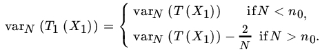
1. Suppose that Tn is a sequence of estimators for parameter θ that satisfies the conditions of Theorem 2. Then , that is, T_n is squared error consistent for θ. If T_n is consistent for θ and for all θ and all (x₁, x₂,…,x_n) ∈ _n, show that . If, however, , then show that T_n may not be squared error consistent for θ.
2. Let X₁,X₂,…,X_n be a sample from . Let . Show that . Write . Is Y_n consistent for θ?
3. Let X₁,X₂,…,X_n be iid RVs with and . Show that is a consistent estimator for μ.
4. Let X₁,X₂,…,X_n be a sample from U[0,θ]. Show that is a consistent estimator for θe^–1.
5. In Problem 2 show that is asymptotically biased for θ and is not BAN. (Show that .)
6. In Problem 5 consider the class of estimators . Show that the estimator in this class has the least MSE.
7. Let X₁, X₂,…,X_n be iid with PDF . Consider the class of estimators . Show that the estimator that has the smallest MSE in this class is given by .

8.3 SUFFICIENCY, COMPLETENESS AND ANCILLARITY

After the completion of any experiment, the job of a statistician is to interpret the data she has collected and to draw some statistically valid conclusions about the population under investigation. The raw data by themselves, besides being costly to store, are not suitable for this purpose. Therefore the statistician would like to condense the data by computing some statistics from them and to base her analysis on these statistics, provided that there is “no loss of information” in doing so. In many problems of statistical inference a function of the observations contains as much information about the unknown parameter as do all the observed values. The following example illustrates this point.

A rigorous definition of the concept involved in the above discussion requires the notion of a conditional distribution and is beyond the scope of this book. In view of the discussion of conditional probability distributions in Section 4.2, the following definition will suffice for our purposes.

Not every statistic is sufficient.

Definition 1 is not a constructive definition since it requires that we first guess a statistic T and then check to see whether T is sufficient. Moreover, the procedure for checking that T is sufficient is quite time-consuming. We now give a criterion for determining sufficient statistics.

We note that the order statistic (X₍₁₎,X₍₂₎,…,X_(n)) is also sufficient. Note also that the parameter is one-dimensional, the statistics (X₍₁₎, X_(n)) is two-dimensional, whereas the order statistic is n-dimensional.

In Example 9 we saw that order statistic is sufficient. This is not a mere coincidence. In fact, if are exchangeable then the joint PDF of X is a symmetric function of its arguments. Thus

and it follows that the order statistic is sufficient for f_θ.

The concept of sufficiency is frequently used with another concept, called completeness, which we now define.

In Definition 3 X will usually be a multiple RV. The family of distributions of T is obtained from the family of distributions of X₁,X₂,…,X_n by the usual transformation technique discussed in Section 4.4.

The next example illustrates the existence of a sufficient statistic which is not complete.

We see by a similar argument that X_(n) is complete, which is the same as saying that is a complete family of densities. Clearly, X_(n) is sufficient.

Using an induction argument, we conclude that and hence . It follows that is a complete family of distributions, and X_(n) is a complete sufficient statistic.

Now suppose that we exclude the value for some fixed from the family . Let us write . Then is not complete. We ask the reader to show that the class of all functions g such that for all consists of functions of the form

where c is a constant, .

Remark 7. Completeness is a property of a family of distributions. In Remark 6 we saw that if a statistic is sufficient for a class of distributions it is sufficient for any subclass of those distributions. Completeness works in the opposite direction. Example 14 shows that the exclusion of even one member from the family destroys completeness.

The following result covers a large class of probability distributions for which a complete sufficient statistic exists.

Let us write ,, and ,. Then , and both are nonnegative functions. In terms of , (3) is the same as

(4)

for all θ.

Let be fixed, and write

(5)

Then both are PMFs, and it follows from (4) that

(6)

for all . By the uniqueness of MGFs (6) implies that

and hence that for all t, which is equivalent to for all t. Since T is clearly sufficient (by the factorization criterion), it is proved that T is a complete sufficient statistic.

In Example 6, 8, and 9 we have shown that a given family of probability distributions that admits a nontrivial sufficient statistic usually admits several sufficient statistics. Clearly we would like to be able to choose the sufficient statistic that results in the greatest reduction of data collection. We next study the notion of a minimal sufficient statistic. For this purpose it is convenient to introduce the notion of a sufficient partition. The reader will recall that a partition of a space is just a collection of disjoint sets E_α such that Any statistic T(X₁,X₂,…,X_n) induces a partition of the space of values of (X₁,X₂,…,X_n), that is, T induces a covering of by a family of disjoint sets , where t belongs to the range of T. The sets A_t are called partition sets. Conversely, given a partition, any assignment of a number to each set so that no two partition sets have the same number assigned defines a statistic. Clearly this function is not, in general, unique.

Let ₁, ₂ be two partitions of a space . We say that ₁ is a subpartition of ₂ if every partition set in ₂ is a union of sets of ₁. We sometimes say also that ₁ is finer than ₂(₂ is coarser than ₁) or that ₂ is a reduction of ₁. In this case, a statistic T₂ that defines ₂ must be a function of any statistic T₁ that defines ₁. Clearly, this function need not have a unique inverse unless the two partitions have exactly the same partition sets.

Given a family of distributions for which a sufficient partition exists, we seek to find a sufficient partition that is as coarse as possible, that is, any reduction of leads to a partition that is not sufficient.

The question of the existence of the minimal partition was settled by Lehmann and Scheffé [65] and, in general, involves measure-theoretic considerations. However, in the cases that we consider where the sample space is either discrete or a finite-dimensional Euclidean space and the family of distributions of X is defined by a family of PDFs (PMFs) such difficulties do not arise. The construction may be described as follows.

Two points x and y in the sample space are said to be likelihood equivalent, and we write , if and only if there exists a which does not depend on θ such that . We leave the reader to check that “~” is an equivalence relation (that is, it is reflexive, symmetric, and transitive) and hence “~” defines a partition of the sample space. This partition defines the minimal sufficient partition.

A rigorous proof of the above assertion is beyond the scope of this book. The basic ideas are outlined in the following theorem.

To prove the sufficiency of the minimal sufficient partition , let T₁ be an RV that induces . Then T₁ takes on distinct values over distinct sets of but remains constant on the same set. If , then

(7)

Now

depending on whether the joint distribution of X is absolutely continuous or discrete. Since f_θ(x)/f_θ(y) is independent of θ whenever , it follows that the ratio on the right-hand side of (7) does not depend on θ. Thus T₁ is sufficient.

In view of Theorem 3 a minimal sufficient statistic is a function of every sufficient statistic. It follows that if T₁ and T₂ are both minimal sufficient, then both must induce the same minimal sufficient partition and hence T₁ and T₂ must be equivalent in the sense that each must be a function of the other (with probability 1).

How does one show that a statistic T is not sufficient for a family of distributions ? Other than using the definition of sufficiency one can sometimes use a result of Lehmann and Scheffé [65] according to which if T₁(X) is sufficient for , then T₂(X) is also sufficient if and only if for some Borel-measurable function g and all , where B is a Borel set with .

Another way to prove T nonsufficient is to show that there exist x for which but x and y are not likelihood equivalent. We refer to Sampson and Spencer [98] for this and other similar results.

The following important result will be proved in the next section.

We emphasize that the converse is not true. A minimal sufficient statistic may not be complete.

If X₁, X₂,…,X_n is a sample from , then (X₍₁₎, X_(n)) is minimal sufficient for θ but not complete since

for all θ.

Finally, we consider statistics that have distributions free of the parameter(s) θ and seem to contain no information about θ. We will see (Example 23) that such statistics can sometimes provide useful information about θ.

In Example 20 we saw that S² was independent of the minimal sufficient statistic . The following result due to Basu shows that it is not a mere coincidence.

The converse of Basu’s Theorem is not true. A statistic S that is independent of every ancillary statistic need not be complete (see, for example, Lehmann [62]).

The following example due to R.A. Fisher shows that if there is no sufficient statistic for θ, but there exists a reasonable statistic not independent of an ancillary statistic A(X), then the recovery of information is sometimes helped by the ancillary statistic via a conditional analysis. Unfortunately, the lack of uniqueness of ancillary statistics creates problems with this conditional analysis.

Consider the statistics

and

Then the joint PDF of S and A is given by

and it is clear that S and A are not independent. The marginal distribution of A is given by the PDF

where C(x, y) is the constant of integration which depends only on x, y, and n but not on θ. In fact, , where K₀ is the standard form of a Bessel function (Watson [116]). Consequently A is ancillary for θ.

Clearly, the conditional PDF of S given is of the form

The amount of information lost by using S(X, Y) alone is th part of the total and this loss of information is gained by the knowledge of the ancillary statistic A(X, Y). These calculations will be discussed in Example 8.5.9.

PROBLEMS 8.3

1. Find a sufficient statistic in each of the following cases based on a random sample of size n:
   1. when (i) α is unknown, β known; (ii) β; is unknown, α known; and (iii) α,β are both unknown.
   2. when (i) α is unknown, β known; (ii) β is unknown, α known; and (iii) α,β are both unknown.
   3. , where
      

      and are integers, when (i) N₁ is known, N₂ unknown; (ii) N₂ known, N₁ unknown; and (iii) N₁,N2 are both unknown.

   4. , where
      
   5. , where
      
   6. , where
      

      and

      
   7. , where
      

      when (i) p is known, θ unknown; (ii) p is unknown, θ known; and (iii) p, θ are both unknown.

2. Let be a sample from (ασ, σ²), where α is a known real number. Show that the statistic is sufficient for σ but that the family of distributions of T(X) is not complete.

   No.

3. Let X₁,X₂,…,X_n be a sample from (μ,σ²). Then is clearly sufficient for the family (μ,σ²), μ∈, . Is the family of distributions of X complete?
4. Let X₁,X₂,…,X_n be a sample from Show that the statistic is sufficient for θ but not complete.
5. If and T is sufficient, then so also is U.
6. In Example 14 show that the class of all functions g for which for all P ∈ consists of functions of the form
   
   where c is a constant.
7. For the class of two DFs where is (0,1) and is (1,0), find a sufficient statistic.
8. Consider the class of hypergeometric probability distributions , where
   

   Show that it is a complete class. If , is complete?

9. Is the family of distributions of the order statistic in sampling from a Poisson distribution complete?
10. Let (X₁,X₂,…,X_n) be a random vector of the discrete type. Is the statistic sufficient?
11. Let X₁,X₂,…,X_n be a random sample from a population with law (X). Find a minimal sufficient statistic in each of the following cases:
    1. .
    2. .
    3. .
    4. .
    5. .
    6. .
    7. .
    8. .
12. Let X₁,X₂ be a sample of size 2 from P(λ). Show that the statistic X₁ + αX₂, where is an integer, is not sufficient for λ.
13. Let X₁, X₂,…,X_n be a sample from the PDF
    

    Show that is a minimal sufficient statistic for θ, but is not sufficient.

14. Let X₁,X₂,…,X_n be a sample from (0,σ²). Show that is a minimal sufficient statistic but is not sufficient for σ².
15. Let X₁,X₂,…,X_n be a sample from PDF . Find a minimal sufficient statistic for (α,β).
16. Let T be a minimal sufficient statistic. Show that a necessary condition for a sufficient statistic U to be complete is that U be minimal.
17. Let X₁,X₂,…,X_n be iid (μ, σ²). Show that (, S²) is independent of each of
18. Let X₁,X₂,…,X_n be iid (θ,1). Show that a necessary and sufficient condition for and to be independent is .
19. Let X₁,X₂,…,X_n be a random sample from . Show that X₍₁₎ is a complete sufficient statistic which is independent of S².
20. Let X₁,X₂,…,X_n be iid RVs with common PDF . Show that X must be independent of every scale-invariant statistic such as
21. Let T₁,T₂ be two statistics with common domain D. Then T₁ is a function of T₂ if and only if
    
22. Let S be the support of f_θ, θ ∈ Ѳ and let T be a statistic such that for some Ѳ₁,Ѳ₂ ∈ Ѳ, and x, y ∈ S, , but . Then show that T is not sufficient for θ.
23. Let X₁,X₂,…,X_n be iid (Ѳ ,1). Use the result in Problem 22 to show that is not sufficient for θ.
24. 1. If T is complete then show that any one-to-one mapping of T is also complete.
    2. Show with the help of an example that a complete statistic is not unique for a family of distributions.

8.4 UNBIASED ESTIMATION

In this section we focus attention on the class of unbiased estimators. We develop a criterion to check if an unbiased estimator is optimal in this class. Using sufficiency and completeness, we describe a method of constructing uniformly minimum variance unbiased estimators.

Note that S is not, in general, unbiased for σ. If X₁,X₂,…,X_n are iid RVs we know that . Therefore,

The bias of S is given by

We note that so that S is asymptotically unbiased for σ.

If T is unbiased for θ, g(T) is not, in general, an unbiased estimator of g(θ) unless g is a linear function.

Let θ be estimable, and let T be an unbiased estimator of θ. Let T₁ be another unbiased estimator of θ, different from T. This means that there exists at least one θ such that . In this case there exist infinitely many unbiased estimators of θ of the form . It is therefore desirable to find a procedure to differentiate among these estimators.

In general, a particular estimator will be better than another for some values of θ and worse for others. Definitions 2 and 3 are special cases of this concept if we restrict attention only to unbiased estimators.

The following result gives a necessary and sufficient condition for an unbiased estimator to be a UMVUE.

Conversely, let (6) hold for some T₀ ε , all θ ε Θ and all v ε ₀, and let T ε . Then , and for every θ

We have

by the Cauchy-Schwarz inequality. If , then and there is nothing to prove. Otherwise

or . Since T is arbitrary, the proof is complete.

Since T₀ and T are both UMVUEs , and it follows that the correlation coefficient between T and T₀ is 1. This implies that for some a, b and all θ ε Θ. Since T and T₀ are both unbiased for θ, we must have for all θ.

Remark 4. Both Theorems 1 and 2 have analogs for LMVUE's at θ₀ ε Θ, θ₀ fixed.

We now turn our attention to some methods for finding UMVUE's.

We will show that . Let . Then Y is (nθ, n), X1 is (θ,1), and (X₁, Y) is a bivariate normal RV with variance covariance matrix . Therefore,

as asserted.

If we let , we can show similarly that is the UMVUE for ψ(θ). Note that may occasionally be negative, so that an UMVUE for θ² is not very sensible in this case.

If we consider the family instead, we have seen (Example 8.3.14 and Problem 8.3.6) that is not complete. The UMVUE for the family is , which is not the UMVUE for . The UMVUE for is in fact, given by

The reader is asked to check that T₁ has covariance 0 with all unbiased estimators g of 0 that are of the form described in Example 8.3.14 and Problem 8.3.6, and hence Theorem 1 implies that T₁ is the UMVUE. Actually T₁(X₁) is a complete sufficient statistic for . Since, is not even unbiased for the family . The minimum variance is given by

The following example shows that UMVUE may exist while minimal sufficient statistic may not.

It follows that , and for . Thus

and so on. Consequently, all unbiased estimators of 0 are of the form . Clearly, if otherwise is unbiased for (θ). Moreover, for all θ

so that T is UMVUE of ψ(θ).

We conclude this section with a proof of Theorem 8.3.4.

PROBLEMS 8.4

1. Let X₁,X₂,…,X_n be a sample from b(1,p). Find an unbiased estimator for .
2. Let X₁,X₂,…,X_n be a sample from (μ,σ²). Find an unbiased estimator for σ^p, where . Find a minimum MSE estimator of σ^p.
3. Let X₁,X₂,…,X_n be iid (μ,σ²) RVs. Find a minimum MSE estimator of the form αS² for the parameter σ². Compare the variances of the minimum MSE estimator and the obvious estimator S².
4. Let . Does there exist an unbiased estimator of θ?
5. Let . Does there exist an unbiased estimator of ?
6. Let X₁,X₂,…,X_n be a sample from be an integer. Find the UMVUE for (a) and (b) .
7. Let X₁,X₂,…,X_n be a sample from a population with mean θ and finite variance, and T be an estimator of θ of the form . If T is an unbiased estimator of θ that has minimum variance and T' is another linear unbiased estimator of θ, then
   
8. Let T₁, T₂ be two unbiased estimators having common variance, , where σ² is the variance of the UMVUE. Show that the correlation coefficient between .
9. Let and . Let X₁,X₂,…,X_n be a sample on X. Find the UMVUE of d(θ).
10. This example covers most discrete distributions. Let X₁,X₂,…,X_n be a sample from PMF
    

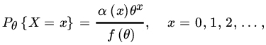
    where , and let . Write

    

    Show that T is a complete sufficient statistic for θ and that the UMVUE for (r > 0 is an integer) is given by

    
    (Roy and Mitra [94])

     

11. Let X be a hypergeometric RV with PMF
    

    where max .

    1. Find the UMVUE for M when N is assumed to be known.
    2. Does there exist an unbiased estimator of N (M known)?
12. Let X₁,X₂,…X_n be iid . Find the UMVUE of , where is a fixed real number.
13. Let X₁,X₂,…,X_n be a random sample from P(λ). Let be a parametric function. Find the UMVUE for ψ(λ). In particular, find the UMVUE for (a) , (b) for some fixed integer , (c) , and (d) .
14. Let X₁,X₂,…,X_n be a sample from PMF
    

    Let ψ(N) be some function of N. Find the UMVUE of ψ(N).

15. Let X₁,X₂,…,X_n be a random sample from P(λ). Find the UMVUE of , where k is a fixed positive integer.
16. Let (X₁,Y₁),(X₂,Y₂),…,(X_n,Y_n) be a sample from a bivariate normal population with parameters , and ρ. Assume that , and it is required to find an unbiased estimator of μ. Since a complete sufficient statistic does not exist, consider the class of all linear unbiased estimators
    
    1. Find the variance of .
    2. Choose to minimize and consider the estimator
       

       Compute . If , the BLUE of μ (in the sense of minimum variance) is

       

       irrespective of whether σ₁ and ρ are known or unknown.

    3. If and ρ, σ₁, σ₂ are unknown, replace these values in α₀ by their corresponding estimators. Let
       

       Show that

       

       is an unbiased estimator of μ.

17. Let X₁,X₂,…,X_n be iid (θ,1). Let , where Φ is the DF of a (0,1) RV. Show that the UMVUE of p is given by .
18. Prove Theorem 5.
19. In Example 10 show that T₁ is the UMVUE for N (restricted to the family ), and compute the minimum variance.
20. Let (X₁,Y₁),…,(X_n,Y_n) be a sample from a bivariate population with finite variances , respectively, and covariance γ. Show that
    

    where . It is assumed that appropriate order moments exist.

21. Suppose that a random sample is taken on (X,Y) and it is desired to estimate γ, the unknown covariance between X and Y. Suppose that for some reason a set S of n observations is available on both X and Y, an additional n₁–n observations are available on X but the corresponding Y values are missing, and an additional n₂ – n observations of Y are available for which the X values are missing. Let S₁ be the set of all X values, and S₂, the set of all Y values, and write
    

    Show that

    

    is an unbiased estimator of γ. Find the variance of , and show that , where S₁₁ is the usual unbiased estimator of γ based on the n observations in S (Boas [11]).

22. Let X₁,X₂,…,X_n be iid with common PDF . Let x₀ be a fixed real number. Find the UMVUE of f_θ(x₀).
23. Let X1,X2,…,X_n be iid (μ,1) RVs. Let . Show that is UMVUE of φ(x;,1) where φ(x;μ,σ²) is the PDF of a RV.
24. Let X1,X2,…,Xn be iid G(1, θ) RVs. Show that the UMVUE of , , is given by h(x|t) the conditional PDF of X₁ given where
    
25. Let X₁,X₂,…,X_n be iid RVs with common PDF , and = 0 elsewhere. Show that is a complete sufficient statistic for θ. Find the UMVU estimator of θ^r.
26. Let X1,X2,…,X_n be a random sample from PDF
    

    where .

    1. is a complete sufficient statistic for θ.
    2. Show that the UMVUEs of μ and σ are given by
       
    3. Find the UMVUE of .
    4. Show that the UMVUE of is given by
       

       where .

8.5 UNBIASED ESTIMATION (CONTINUED): A LOWER BOUND FOR THE VARIANCE OF AN ESTIMATOR

In this section we consider two inequalities, each of which provides a lower bound for the variance of an estimator. These inequalities can sometimes be used to show that an unbiased estimator is the UMVUE. We first consider an inequality due to Fréchet, Cramér, and Rao (the FCR inequality).

Let (p) be a function of p and T(X) be an unbiased estimator of (p). The only condition that need be checked is differentiability under the summation sign. We have

which is a polynomial in p and hence can be differentiated with respect to p. For any unbiased estimator T(X) of p we have

and since

it follows that the variance of the estimator X/n attains the lower bound of the FCR inequality, and hence T(X) has least variance among all unbiased estimators of p. Thus T(X) is UMVUE for p.

Let us next consider the problem of unbiased estimation of based on a sample of size 1. The estimator

is unbiased for ψ(λ) since

Also,

To compute the FCR lower bound we have

This has to be differentiated with respect to , since we want a lower bound for an estimator of the parameter . Let . Then

and

so that

where .

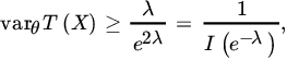
Since for , we see that var(δ(X)) is greater than the lower bound obtained from the FCR inequality. We show next that δ(X) is the only unbiased estimator of θ and hence is the UMVUE.

If h is any unbiased estimator of θ, it must satisfy . That is, for all

Equating coefficients of powers of λ we see immediately that and for . It follows that .

The same computation can be carried out when X₁,X₂,…,X_n is random sample from P(λ). We leave the reader to show that the FCR lower bound for any unbiased estimator of is . The estimator is clearly unbiased for with variance . The UMVUE of is given by with .

Corollary. Let X₁,X₂,…,X_n be iid with common PDF f_θ(x). Suppose the family satisfies the conditions of Theorem 1. Then equality holds in (2) if and only if, for all ,

(8)

for some function k(θ).

Proof. Recall that we derived (2) by an application of Cauchy–Schwatz inequality where equality holds if and only if (8) holds.

Remark 7. Integrating (8) with respect to θ we get

for some functions , S, and A. It follows that f_θ is a one-parameter exponential family and the statistic T is sufficient for θ.

Remark 8. A result that simplifies computations is the following. If f_θ is twice differentiable and can be differentiated under the expectation sign, then

(9)

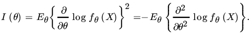
For the proof of (9), it is striaghtforward to check that

Taking expectations on both side we get (9).

We next consider an inequality due to Chapman, Robbins, and Kiefer (the CRK inequality) that gives a lower bound for the variance of an estimator but does not require regularity conditions of the Fréchet-Cramér-Rao type.

We next introduce the concept of efficiency.

It is usual to consider the performance of an unbiased estimator by comparing its variance with the lower bound given by the FCR inequality.

In view of Remarks 6 and 7, the following result describes the relationship between most efficient unbiased estimators and UMVUEs.

Clearly, an estimator T satisfying the conditions of Theorem 3 will be UMVUE, and two estimators coincide. We emphasize that we have assumed the regularity conditions of FCR inequality in making this statement.

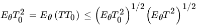
We return to Example 8.3.23 where X₁, X₂,…,X_n are iid G(1, θ), and Y₁,Y₂,…,Y_n iid G(1, 1/θ), and X’s and Y’s are independent. Then (X₁, Y₁) has common PDF f_θ(x, y) given above. We will compute Fisher’s Information for θ in the family of PDFs of . Using the PDFs of and and the transformation technique, it is easy to see that S(X,Y) has PDF

Thus

It follows that

That is, the information about θ in S is smaller than that in the sample.

The Fisher Information in the conditional PDF of S given , where , can be shown (Problem 12) to equal

where K₀ and K₁ are Bessel functions of order 0 and 1, respectively. Averaging over all values of A, one can show that the information is 2n/θ² which is the total Fisher information in the sample of n pairs (x_j, y_j)’s.

PROBLEMS 8.5

1. Are the following families of distributions regular in the sense of Fréchet, Cramér, and Rao? If so, find the lower bound for the variance of an unbiased estimator based on a sample size n.
   1. if , and = 0 otherwise; .
   2. if , and = 0 otherwise.
   3. .
   4. .
2. Find the CRK lower bound for the variance of an unbiased estimator of θ, based on a sample of size n from the PDF of Problem 1(b).
3. Find the CRK bound for the variance of an unbiased estimator of θ in sampling from (θ,1).
4. In Problem 1 check to see whether there exists a most efficient estimator in each case.
5. Let X₁, X₂,…,X_n be a sample from a three-point distribution:
   

   where Does the FCR inequality apply in this case? If so, what is the lower bound for the variance of an unbiased estimator of θ?

   

6. Let X₁, X₂,…,X_n be iid RVs with mean μ and finite variance. What is the efficiency of the unbiased (and consistent) estimator relative to ?
7. When does the equality hold in the CRK inequality?
8. Let X₁, X₂,…,X_n be a sample from (μ, 1), and let :
   1. Show that the minimum variance of any estimator of μ² from the FCR inequality is 4μ²/n:
   2. Show that is the UMVUE of μ² with variance .
9. Let X₁, X₂,…,X_n be iid G(1, 1/α) RVs:
   1. Show that the estimator is the UMVUE for α with variance .
   2. Show that the minimum variance from FCR inequality is α²/n.
10. In Problem 8.4.16 compute the relative efficiency of with respect to .
11. Let X₁,X₂,…,X_n and Y₁,Y₂,…,Y_m be independent samples from and , respectively, where are unknown. Let and , and consider the problem of unbiased estimation of μ:
    1. If ρ is known, show that
       

       where is the BLUE of μ. Compute .

    2. If ρ is unknown, the unbiased estimator
       

       is optimum in the neighborhood of . Find the variance of .

    3. Compute the efficiency of relative to .
    4. Another unbiased estimator of μ is
       

       where is an RV.

12. Show that the Fisher Information on θ based on the PDF
    

    for fixed a equals , where K₀(2a) and K₁(2a) are Bessel functions of order 0 and 1 respectively.

8.6 SUBSTITUTION PRINCIPLE (METHOD OF MOMENTS)

One of the simplest and oldest methods of estimation is the substitution principle: Let ψ(θ), θ ∈ Θ be a parametric function to be estimated on the basis of a random sample X₁, X₂,…, X_n from a population DF F. Suppose we can write for some known function h. Then the substitution principle estimator of ψ(θ) is . where is the sample distribution function. Accordingly we estimate by by , and so on. The method of moments is a special case when we need to estimate some known function of a finite number of unknown moments. Let us suppose that we are interested in estimating

(1)

where h is some known numerical function and m_j is the jth-order moment of the population distribution that is known to exist for .

Remark 1. It is easy to extend the method to the estimation of joint moments. Thus we use to estimate E(XY) and so on.

Remark 2. From the WLLN, . Thus, if one is interested in estimating the population moments, the method of moments leads to consistent and unbiased estimators. Moreover, the method of moments estimators in this case are asymptotically normally distributed (see Section 7.5).

Again, if one estimates parameters of the type θ defined in (1) and h is a continuous function, the estimators T(X_1,X₂,…, X_n) defined in (2) are consistent for θ (see Problem 1). Under some mild conditions on h, the estimator T is also asymptotically normal (see Cramér [17, pp. 386–387]).

In particular, if X₁, X₂,…, X_n are iid P(λ) RVs, we know that and . The method of moments leads to using either or as an estimator of λ. To avoid this kind of ambiguity we take the estimator involving the lowest-order sample moment.

Method of moments may lead to absurd estimators. The reader is asked to compute estimators of θ in (θ, θ) or (θ, θ²) by the method of moments and verify this assertion.

PROBLEMS 8.6

1. Let , and , where a and b are constants. Let be a continuous function. Show that .
2. Let X₁, X₂,…, X_n be a sample from G(α, β). Find the method of moments estimator for (α, β).
3. Let X₁, X₂,…, X_n be a sample from (μ, σ²). Find the method of moments estimator for (μ, σ²).
4. Let X₁, X₂,…, X_n be a sample from B(α, β). Find the method of moments estimator for (α, β).
5. A random sample of size n is taken from the lognormal PDF
   

   Find the method of moments estimators for μ and σ².

8.7 MAXIMUM LIKELIHOOD ESTIMATORS

In this section we study a frequently used method of estimation, namely, the method of maximum likelihood estimation. Consider the following example.

The principle of maximum likelihood essentially assumes that the sample is representative of the population and chooses as the estimator that value of the parameter which maximizes the PDF (PMF) f_θ(x).

Usually θ will be a multiple parameter. If X_1; X₂,…, X_n are iid with PDF (PMF) f_θ(x), the likelihood function is

(2)

Let and .

It is convenient to work with the logarithm of the likelihood function. Since log is a monotone function,

(4)

Let Θ be an open subset of _k, and suppose that f_θ(x) is a positive, differentiable function of (that is, the first-order partial derivatives exist in the components of θ). If a supremum exists, it must satisfy the likelihood equations

(5)

Any nontrivial root of the likelihood equations (5) is called an MLE in the loose sense. A parameter value that provides the absolute maximum of the likelihood function is called an MLE in the strict sense or, simply, an MLE.

Remark 1. If , there may still be many problems. Often the likelihood equation has more than one root, or the likelihood function is not differentiable everywhere in Θ, or may be a terminal value. Sometimes the likelihood equation may be quite complicated and difficult to solve explicitly. In that case one may have to resort to some numerical procedure to obtain the estimator. Similar remarks apply to the multiparameter case.

Note that is not unbiased for σ² Indeed, . But is unbiased, as we already know. Also, is unbiased, and both and are consistent. In addition, and are method of moments estimators for μ and σ² and is jointly sufficient.

Finally, note that is the MLE of μ if σ² is known; but if f is known, the MLE of σ² a² is not but

We see that the MLE is consistent, sufficient, and complete, but not unbiased.

In particular, let and and suppose that the observations, arranged in increasing order of magnitude, are 1, 2, 4. In this case the MLE can be shown to be , which corresponds to the first-order statistic. If the sample values are 2, 3, 4, the third-order statistic is the MLE.

Remark 2. We have seen that MLEs may not be unique, although frequently they are. Also, they are not necessarily unbiased even if a unique MLE exists. In terms of MSE, an MLE may be worthless. Moreover, MLEs may not even exist. We have also seen that MLEs are functions of sufficient statistics. This is a general result, which we now prove.

Let us write . Then

so that

We need only to show that .

Recall from (8.5.4) with that

and substituting we get

That is,

and the proof is complete.

Remark 3. In Theorem 2 we assumed the differentiability of A(θ) and the existence of the second-order partial derivative . If the conditions of Theorem 2 are satisfied, the most efficient estimator is necessarily the MLE. It does not follow, however, that every MLE is most efficient. For example, in sampling from a normal population, is the MLE of σ², but it is not most efficient. Since is , we see that , which is not equal to the FCR lower bound, 2σ⁴/n. Note that is not even an unbiased estimator of σ².

We next consider an important property of MLEs that is not shared by other methods of estimation. Often the parameter of interest is not θ but some function h(θ).If is MLE of θ what is the MLE of h(θ)? If is a one to one function of θ, then the inverse function is well defined and we can write the likelihood function as a function of λ We have

so that

It follows that the supremum of L^* is achieved at . Thus is the MLE of h (θ).

In many applications is not one-to-one. It is still tempting to take as the MLE of λ. The following result provides a justification.

Let , so that . Therefore, the MLE of β is M/log , where is the MLE of p. To compute the MLE of p we have

so that the MLE of p is . Thus the MLE of β is

Finally we consider some important large-sample properties of MLE's. In the following we assume that is a family of PDFs (PMFs), where Θ is an open interval on . The conditions listed below are stated when f_θ is a PDF. Modifications for the case where f_θ is a PMF are obvious and will be left to the reader.

1. exist for all θ ε Θ and every x. Also,
   
2. for all θ ε Θ.
3. for all θ
4. There exists a function H(x) such that for all θ ε Θ
   
5. There exists a function g(θ) which is positive and twice differentiable for every θεΘ, and a function H(x) such that for all θ
   

Note that the condition (v) is equivalent to condition (iv) with the added qualification that .

We state the following results without proof.

On occasions one encounters examples where the conditions of Theorem 4 are not satisfied and yet a solution of the likelihood equation is consistent and asymptotically normal.

The following theorem covers such cases also.

Remark 4. It is important to note that the results in Theorems 4 and 5 establish the consistency of some root of the likelihood equation but not necessarily that of the MLE when the likelihood equation has several roots. Huzurbazar [47] has shown that under certain conditions the likelihood equation has at most one consistent solution and that the likelihood function has a relative maximum for such a solution. Since there may be several solutions for which the likelihood function has relative maxima, Cramér's and Huzurbazar's results still do not imply that a solution of the likelihood equation that makes the likelihood function an absolute maximum is necessarily consistent.

Wald [115] has shown that under certain conditions the MLE is strongly consistent. It is important to note that Wald does not make any differentiability assumptions.

In any event, if the MLE is a unique solution of the likelihood equation, we can use Theorems 4 and 5 to conclude that it is consistent and asymptotically normal. Note that the asymptotic variance is the same as the lower bound of the FCR inequality.

We leave the reader to check that in Example 13 conditions of Theorem 5 are satisfied.

Remark 5. The invariance and the large sample properties of MLEs permit us to find MLEs of parametric functions and their limiting distributions. The delta method introduced in Section 7.5 (Theorem 1) comes in handy in these applications. Suppose in Example 13 we wish to estimate . By invariance of MLEs, the MLE of where is the MLE of θ. Applying Theorem 7.5.1 we see that is AN(θ², 8θ⁴/n).

In Example 14, suppose we wish to estimate Then is the MLE of ψ(λ) and, in view of Theorem 7.5.1, .

Remark 6. Neither Theorem 4 nor Theorem 5 guarantee asymptotic normality for a unique MLE. Consider, for example, a random sample from U(0,θ]. Then X_(n) is the unique MLE for θ and in Problem 8.2.5 we asked the reader to show that .

PROBLEMS 8.7

1. Let X₁, X₂,…,X_n be iid RVs with common PMF (pdf) f_θ (x).Find an MLE for θ in each of the following cases:
   1. 
   2. .
   3. and ∝ known.
   4. .
2. Find an MLE, if it exists, in each of the following cases:
   1. : both n and are unknown, and one observation is available.
   2. .
   3. .
   4. X₁, X₂, …, X_n is a sample from
      
   5. .
   6. .
3. Suppose that n observations are taken on an RV X with distribution (μ,1), but instead of recording all the observations one notes only whether or not the observation is less than 0. If occurs times, find the MLE of μ.
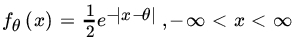
4. Let X₁, X₂ ,…,X_n be a random sample from PDF
   
   1. Find the MLE of (α, β).
   2. Find the MLE of .
5. Let X₁, X₂,…,X_n be a sample from exponential density , . Find the MLE of θ, and show that it is consistent and asymptotically normal.
6. For Problem 8.6.5 find the MLE for (μ, σ²).
7. For a sample of size 1 taken from (μ, σ²), show that no MLE of (μ, σ²) exists.
8. For Problem 8.6.5 suppose that we wish to estimate N on the basis of observations X_1,X₂,…, X_M:
   1. Find the UMVUE of N.
   2. Find the MLE of N.
   3. Compare the MSEs of the UMVUE and the MLE.
9. Let be independent RVs where , Find MLEs for μ₁, μ₂, …, μ_s, and σ². Show that the MLE for σ² is not consistent as s →∞ (n fixed) (Neyman and Scott [77]).
10. Let (X, Y) have a bivariate normal distribution with parameters , and p Suppose that n observations are made on the pair (X,Y), and N–n observations on X that is, N–n observations on Y are missing. Find the MLE's of μ₁, μ₂, σ²₁σ²₂, and p (Anderson [2] ).

    [Hint: If is the joint PDF of (X,Y) write

    

    where f₁ is the marginal (normal) PDF of X, and f_Y|X is the conditional (normal) PDF of Y, given x with mean

    

    and variance . Maximize the likelihood function first with respect to μ₁ and and then with respect to , and

11. In Problem 5, let denote the MLE of θ. Find the MLE of asymptotic distribution.
12. In Problem 1(d), find the asymptotic distribution of the MLE of θ.
13. In Problem 2(a), find MLE of and its asymptotic distribution.
14. Let X₁,X₂,…, X_n, be a random sample from some DF F on the real line. Suppose we observe x₁,x₂,…,x_n which are all different. Show that the MLE of F is , the empirical DF of the sample.
15. Let X₁, X₂, …, X_n be iid (μ,1). Suppose . Find the MLE of μ
16. Let have a multinomial distribution with parameters , , , where n is known. Find the MLE of .

    .

17. Consider the one parameter exponential density introduced in Section 5.5 in its natural form with PDF
    
    1. Show that the MGF of T(X) is given by
       
       for t in some neighborhood of the origin. Moreover, and .
    2. If the equation has a solution, it must be the unique MLE of η.
18. In Problem 1(b) show that the unique MLE of θ is consistent. Is it asymptotically normal?

8.8 BAYES AND MINIMAX ESTIMATION

In this section we consider the problem of point estimation in a decision-theoretic setting. We will consider here Bayes and minimax estimation.

Let be a family of PDFs (PMFs) and X₁, X₂,…,X_n be a sample from this distribution. Once the sample point (x₁, x₂,…,x_n) is observed, the statistician takes an action on the basis of these data. Let us denote by the set of all actions or decisions open to the statistician.

If is observed, the statistician takes action

Another element of decision theory is the specification of a loss function, which measures the loss incurred when we take a decision.

The value L(θ, a) is the loss to the statistician if he takes action a when θ is the true parameter value. If we use the decision function δ(X) and loss function L and θ is the true parameter value, then the loss is the RV L(θ, δ(X)). (As always, we will assume that L is a Borel-measurable function.)

The basic problem of decision theory is the following: Given a space of actions A, and a loss function L(θ, a), find a decision function δ in D such that the risk R(θ, δ) is "minimum" in some sense for all . We need first to specify some criterion for comparing the decision functions δ.

If the problem is one of estimation, that is, if , we call δ* satisfying (2) a minimax estimator of θ.

The computation of minimax estimators is facilitated by the use of the Bayes estimation method. So far, we have considered θ as a fixed constant and f_θ(x) has represented the PDF (PMF) of the RV X. In Bayesian estimation we treat θ as a random variable distributed according to PDF (PMF) π(θ) on Θ.Also, π is called the a priori distribution.Now represents the conditional probability density (or mass) function of RV X, given that is held fixed. Since π is the distribution of θ, it follows that the joint density (PMF) of θ and X is given by

(3)

In this framework R(θ, δ) is the conditional average loss, , given that θ is held fixed. (Note that we are using the same symbol to denote the RV θ and a value assumed by it.)

Remark 1. The argument used in Theorem 1 shows that a Bayes estimator is one which minimizes . Theorem 1 is a special case which says that if the function

is the Bayes estimator for θ with respect to π, the a priori distribution on Θ.

Remark 2. Suppose T(X) is sufficient for the parameter θ. Then it is easily seen that the posterior distribution of θ given x depends on x only through T and it follows that the Bayes estimator of θ is a function of T.

The quadratic loss function used in Theorem 1 is but one example of a loss function in frequent use. Some of many other loss functions that may be used are

Clearly δ* is also the Bayes estimator under the quadratic loss function .

Key to the derivation of Bayes estimator is the posteriori distribution, h(θ | x).The derivation of the posteriori distribution, however, is a three-step process:

1. Find the joint distribution of X and θ given by .
2. Find the marginal distribution with PDF (PMF) g(x) by integrating (summing) over
3. Divide the joint PDF (PMF) by g(x).

It is not always easy to go through these steps in practice. It may not be possible to obtain in a closed form.

To avoid problem of integration such as that in Example 8, statisticians use the so-called conjugate prior distributions. Often there is a natural parameter family of distributions such that the posterior distributions also belong to the same family. These priors make the computations much easier.

Conjugate priors are popular because whenever the prior family is parametric the posterior distributions are always computable, being an updated parametric version of π(θ). One no longer needs to go through a computation of g, the marginal PDF (PMF) of X.Once is known g, if needed, is easily determined from

Thus in Example 10, we see easily that g(x) is beta while in Example 6 g is given by

Conjugate priors are usually associated with a wide class of sampling distributions, namely, the exponential family of distributions.

Natural Conjugate Priors
Smapling PDF(PMF),	Prior π(θ)	Posterior
N(θ, σ2)	N(μ, τ2)
G(v, β)	G(α, β)
b(n, p)	B(α, β)
P(λ)	G(α, β)
NB(r; p)	B(α, β)
G(γ, 1/θ)	G(α, β)

Another easy way is to use a noninformative prior π(θ) though one needs some integration to obtain g(x).

Calculation of becomes easier by-passing the calculation of g(x) when is invariant under a group of transformations following Fraser’s [33] structural theory.

Let be a group of Borel-measurable functions on _n onto itself. The group operation is composition, that is, if g₁ and g₂ are mappings from _n onto _n, g₂g₁ is defined by . Also, is closed under composition and inverse, so that all maps in are one-to-one. We define the group G of affine linear transformations by

The inverse of {a, b} is

and the composition {a, b} and is given by

In particular,

The following theorem provides a method for determining minimax estimators.

The following examples show how to obtain constant risk estimators and the suitable prior distribution.

Consider the natural conjugate priori PDF

The a posteriori PDF of p. given x, is expressed by

It follows that

Which is the Bayes estimator for a squared error loss .For this to be of the form δ*, we must have

giving . It follows that the estimator δ*(x) is minimax with constant risk

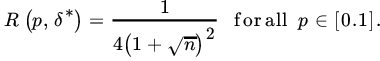
Note that the UMVUE (which is also the MLE) is with risk . Comparing the two risks (Figs. 1 and 2), we see that

so that

in the interval , where as . Moreover,

Clearly, we would prefer the minimax estimator if n is small and would prefer the UMVUE because of its simplicity if n is large.

The following theorem which is an extension of Theorem 2 is of considerable help to prove minimaxity of various estimators.

Proof. Clearly, . Suppose is not admissible, then there exists another rule δ*(x) such that while the inequality is strict for some (say). Now, the risk R(θ, δ) is a continuous function of θ and hence there exists an such that . for .

Now consider the prior N(0, τ²). Then the Bayes estimator is ith risk . Thus,

However,

We get

The right-hand side goes to . This result leads to a contradiction that δ* is admissible. Hence is admissible under squared loss.

Thus we have proved that is an admissible minimax estimator of the mean of a normal distribution .

PROBLEMS 8.8

1. It rains quite often in Bowling Green, Ohio. On a rainy day a teacher has essentially three choices: (1) to take an umbrella and face the possible prospect of carrying it around in the sunshine; (2) to leave the umbrella at home and perhaps get drenched; or (3) to just give up the lecture and stay at home. Let , where θ₁ corresponds to rain, and θ₂, to no rain. Let , where a_i corresponds to the choice i, . Suppose that the following table gives the losses for the decision problem:

   	θ1	θ2
   a1	1	2
   a2	4	0
   a3	5	5

   The teacher has to make a decision on the basis of a weather report that depends on θ as follows.

   	θ1	θ2
   W1 (Rain)	0.7	0.2
   W2 (No Rain)	0.3	0.8

   Find the minimax rule to help the teacher reach a decision.

2. Let X₁,X₂,…, X_n be a random sample from P(λ). For estimating λ, using the quadratic error loss function, an a priori distribution over Θ, given by PDF
   

   is used:

   1. Find the Bayes estimator for λ.
   2. If it is required to estimate with the same loss function and same a priori PDF, find the Bayes estimator for ϕ(λ).
3. Let X₁, X₂,…, X_n be a sample from b(1, θ). Consider the class of decision rules δ of the form , where α is a constant to be determined. Find α according to the minimax principle, using the loss function (θ–δ)², where δ is an estimator for θ.
4. Let δ* be a minimax estimator for aψ(θ) with respect to the squared error loss function. Show that is a minimax estimator for .
5. Let , and suppose that the a priori PDF of θ is U(0, 1). Find the Bayes estimator of θ, using loss function . Find a minimax estimator for θ.
6. In Example 5 find the Bayes estimator for p².
7. Let X₁, X₂,…, X_n be a random sample from G(1, 1/λ). To estimate λ, let the a priori PDF on λ be , and let the loss function be squared error. Find the Bayes estimator of λ.
8. Let X₁, X₂,…, X_n be iid U(0, θ) RVs. Suppose the prior distribution of θ is a Pareto PDF . Using the quadratic loss function find the Bayes estimator of θ.
9. Let T be the unique Bayes estimator of θ with respect to the prior density π. Then T is admissible.
10. Let X₁, X₂,…, X_n be iid with PDF . Take . Find the Bayes estimator of θ under quadratic loss.
11. For the PDF of Problem 10 consider the estimation of θ under quadratic loss. Consider the class of estimators a for all . Show that X₍₁₎–1/n is minimax in this class.

8.9 PRINCIPLE OF EQUIVARIANCE

Let .be a family of distributions of some RV X. Let be sample space of values of X. In Section 8.8 we saw that the statistical decision theory revolves around the following four basic elements: the parameter space Θ, the action space , the sample space X, and the loss function L(θ, a).

Let be a group of transformations which map X onto itself. We say that is invariant under if for each and every , there is a unique such that whenvever . Accordingly,

(1)

for all Borel subsets in _n. We note that the invariance of under does not change the class of distributions we begin with; it only changes the parameter or index θ to .The group induces , a group of transformations on Θ onto itself.

In order to apply invariance considerations to a decision problem we need also to ensure that the loss function is invariant.

Suppose θ is the mean of PDF f_θ, , and {f_θ} is invariant under . Consider the estimator . What we want in an estimator of θ is that it changes in the same prescribed way as the data are changed. In our case, since X changes to we would like to transform to .

Indeed g on S induces on Θ. Thus if , then so if δ(X) estimates θ then δ(gX) should estimate . The principle of equivariance requires that we restrict attention to equivariant estimators and select the “best” estimator in this class in a sense to be described later in this section.

In Example 6 consider the statistic . Note that under the translation group and . That is, for every . A statistic is said to be invariant under a group of transformations if . for all . When is the translation group, an invariant statistic (function) under is called location-invariant. Similarly if is the scale group, we call scale-invariant and if is the location-scale group, we call location-scale invariant. In Example 6 is location-invariant but not equivariant, and ₂ and are not location-invariant.

A very important property of equivariant estimators is that their risk function is constant on orbits of θ.

Remark 1. When the risk function of every equivariant estimator is constant, an estimator (in the class equivariant estimators) which is obtained by minimizing the constant is called the minimum risk equivariant (MRE) estimator.

Next consider estimation of σ² with and . Then is an equivariant estimator of σ². Note that may be used to designate x on its orbits

Again A(x) is invariant under and A(X) is ancillary to σ². Moreover, , and A(X) are independent.

Finally, we consider estimation of (μ, σ²) when . Then , where is an equivariant estimator of (μ, σ²). Also may be used to designate x on its orbits

Note that the statistic A(X)defined in each of the three cases considered in Example 8 is constant on its orbits. A statistic A is said to be maximal invariant if

1. A is invariant, and
2. A is maximal, that is, for some .

We now derive an explicit expression for MRE estimator for a location parameter. Let X₁, X₂,…, X_n be iid with common PDF . Then is invariant under and an estimator of θ is equivariant if

for all real b.

From Theorem 1 the risk function of an equivariant estimator ∂ is constant with risk

where the expectation is with respect to PDF . Consequently, among all equivariant estimators ∂ for θ, the MRE estimator is ∂₀ satisfying

Thus we only need to choose the function q in (4).

Let L(θ, ∂) be the loss function. Invariance considerations require that

for all real b so that L(θ, ∂) must be some function w of

Let , and g(y) be the joint PDF of Y under . Let be the conditional density, under , of X₁ given . Then

(5)

Then R(0, ∂) will be minimized by choosing, for each fixed y, q(y) to be that value of c which minimizes

(6)

Necessarily q depends on y. In the special case , the integral in (6) is minimum when c is chosen to be the mean of the conditional distribution. Thus the unique MRE estimator of θ is given by

(7)

This is the so-called Pitman estimator. Let us simplify it a little more by computing .

First we need to compute h(u|y). When , the joint PDF of X₁, Y₂,…, Y_n is easily seen to be

so the joint PDF of (Y₂,…, Y_n) is given by

It follows that

(8)

Now let . Then the conditional PDF of Z given y is . It follows from (8) that

(9)

Remark 2. Since the joint PDF of X₁, X₂,…, X_n is , the joint PDF of θ and X when θ has prior π(θ) is . The joint marginal of X is . It follows that the conditional pdf of θ given is given by

Taking , the improper uniform prior on Θ, we see from (9) that ∂₀(x) is the Bayes estimator of θ under squared error loss and prior . Since the risk of ∂₀ is constant, it follows that ∂₀ is also minimax estimator of θ.

Remark 3. Suppose S is sufficient for θ. Then . so that the Pitman estimator of θ can be rewritten as

which is a function of s alone.

We now consider, briefly, Pitman estimator of a scale parameter. Let X have a joint PDF

where f is known and is a scale parameter. The family remains invariant under which induces on Θ. Then for estimation of σ^k loss function L(σ, a) is invariant under these transformations if and only if . An estimator ∂ of σ^k is equivariant under if

Some simple examples of scale-equivariant estimators of σ are the mean deviation and the standard deviation . We note that the group over Θ is transitive so according to Theorem 1, the risk of any equivariant estimator of σ^k is free of σ and an MRE estimator minimizes this risk over the class of all equivariant estimators of σ^k. Using the loss function it can be shown that the MRE estimator of σ^k, also known as the Pitman estimate of σ^k, is given by

Just as in the location case one can show that ∂₀ is a function of the minimal sufficient statistic and ∂₀ is the Bayes estimator of σ^k with improper prior . Consequently, ∂₀ is minimax.

PROBLEMS 8.9

In all problems assume that X₁, X₂,…, X_n is a random sample from the distribution under consideration.

1. Show that the following statistics are equivariant under translation group:
   1. Median (X_i).
   2. .
   3. , the quantile of order p, .
   4. .
   5. , where is the mean of a sample of size m, .
2. Show that the following statistics are invariant under location or scale or location scale group:
   1. – median (X_i).
   2. .
   3. .
   4. , where (X₁, Y₁,…,(X_n, Y_n) is random sample from a bivariate distribution.
3. Let the common distribution be G(α, σ) where is known and is unknown. Find the MRE estimator of σ under loss .
4. Let the common PDF be the folded normal distribution
   

   Verify that the best equivariant estimator of μ under quadratic loss of given by

   
5. Let .
   1. Show that (X₍₁₎, X_(n)) is jointly sufficient statistic for θ.
   2. Verify whether or not (X_(n)–X₍₁₎) is an unbiased estimator of θ. Find an ancillary statistic.
   3. Determine the best invariant estimator of θ under loss function .
6. Let
   

   Find the Pitman estimator of θ.

7. Let , for . Find the Pitman estimator of θ.
8. Show that an estimator or ∂ is (location) equivariant if and only if
   

   Where ∂₀ is any equivariant estimator and φ is an invariant function.

9. Let X₁, X₂ be iid with PDF
   

   Find, explicitly, the Pitman estimator of σ^r.

10. Let X₁, X₂,…,X_n be iid with PDF
    

    Find the Pitman estimator of θ^k.