10
SOME FURTHER RESULTS ON HYPOTHESES TESTING
10.1 INTRODUCTION
In this chapter we study some commonly used procedures in the theory of testing of hypotheses. In Section 10.2 we describe the classical procedure for constructing tests based on likelihood ratios. This method is sufficiently general to apply to multi-parameter problems and is specially useful in the presence of nuisance parameters. These are unknown parameters in the model which are of no inferential interest. Most of the normal theory tests described in Sections 10.3 to 10.5 and those in Chapter 12 can be derived by using methods of Section 10.2. In Sections 10.3 to 10.5 we list some commonly used normal theory-based tests. In Section 10.3 we also deal with goodness-of-fit tests. In Section 10.6 we look at the hypothesis testing problem from a decision-theoretic viewpoint and describe Bayes and minimax tests.
10.2 GENERALIZED LIKELIHOOD RATIO TESTS
In Chapter 9 we saw that UMP tests do not exist for some problems of hypothesis testing. It was suggested that we restrict attention to smaller classes of tests and seek UMP tests in these subclasses or, alternatively, seek tests which are optimal against local alternatives. Unfortunately, some of the reductions suggested in Chapter 9, such as invariance, do not apply to all families of distributions.
In this section we consider a classical procedure for constructing tests that has some intuitive appeal and that frequently, though not necessarily, leads to optimal tests. Also, the procedure leads to tests that have some desirable large-sample properties.
Recall that for testing ![]() against
against ![]() , Neyman-Pearson MP test is based on the ratio f1(x)/f0(x). If we interpret the numerator as the best possible explanation of x under H1 and the denominator as the best possible explanation of X under H0, then it is reasonable to consider the ratio
, Neyman-Pearson MP test is based on the ratio f1(x)/f0(x). If we interpret the numerator as the best possible explanation of x under H1 and the denominator as the best possible explanation of X under H0, then it is reasonable to consider the ratio

as a test statistic for testing ![]() against
against ![]() . Here L(θ; x) is the likelihood function of x. Note that for each x for which the MLEs of θ under Θ1 and Θ0 exist the ratio is well defined and free of θ and can be used as a test statistic. Clearly we should reject H0 if
. Here L(θ; x) is the likelihood function of x. Note that for each x for which the MLEs of θ under Θ1 and Θ0 exist the ratio is well defined and free of θ and can be used as a test statistic. Clearly we should reject H0 if ![]() .
.
The statistic r is hard to compute; only one of the two supremas in the ratio may be attained.
Let ![]() be a vector of parameters, and let X be a random vector with PDF (PMF) fθ. Consider the problem of testing the null hypothesis
be a vector of parameters, and let X be a random vector with PDF (PMF) fθ. Consider the problem of testing the null hypothesis ![]() against the alternative
against the alternative ![]() .
.
We leave the reader to show that the statistics λ(X) and r(X) lead to the same criterion for rejecting H0.
The numerator of the likelihood ratio λ is the best explanation of X (in the sense of maximum likelihood) that the null hypothesis H0 can provide, and the denominator is the best possible explanation of X. H0 is rejected if there is a much better explanation of X than the best one provided by H0.
It is clear that ![]() . The constant c is determined from the size restriction
. The constant c is determined from the size restriction
If the distribution of λ is continuous (that is, the DF is absolutely continuous), any size α is attainable. If, however, λ(X) is a discrete RV, it may not be possible to find a likelihood ratio test whose size exactly equals α. This problem arises because of the nonrandomized nature of the likelihood ratio test and can be handled by randomization. The following result holds.
The GLR test is of the type obtained in Section 9.4 for families with an MLR except for the boundary ![]() . In other words, if the size of the test happens to be exactly α, the likelihood ratio test is a UMP level α test. Since X is a discrete RV, however, to obtain size α may not be possible. We have
. In other words, if the size of the test happens to be exactly α, the likelihood ratio test is a UMP level α test. Since X is a discrete RV, however, to obtain size α may not be possible. We have
If such a c′ does not exist, we choose an integer c′ such that
The situation in Example 1 is not unique. For one-parameter exponential family it can be shown (Birkes [7]) that a GLR test of ![]() against
against ![]() is UMP of its size. The result holds also for the dual
is UMP of its size. The result holds also for the dual ![]() and, in fact, for a much wider class of one-parameter family of distributions.
and, in fact, for a much wider class of one-parameter family of distributions.
The GLR test is specially useful when θ is a multiparameter and we wish to test hypothesis concerning one of the parameters. The remaining parameters act as nuisance parameters.
The computations in Example 2 could be slightly simplified by using Theorem 2. Indeed ![]() is a minimal sufficient statistic for θ and since
is a minimal sufficient statistic for θ and since ![]() and S2 are independent the likelihood is the product of the PDFs of
and S2 are independent the likelihood is the product of the PDFs of ![]() and S2. We note that
and S2. We note that ![]() and
and ![]() . We leave it to the reader to carry out the details.
. We leave it to the reader to carry out the details.
In Example 3 we can obtain the same GLR test by focusing attention on the joint sufficient statistic ![]() where
where ![]() and
and ![]() are sample variances of the X’s and the Y’s, respectively. In order to write down the likelihood function we note that
are sample variances of the X’s and the Y’s, respectively. In order to write down the likelihood function we note that ![]() are independent RVs. The distributions
are independent RVs. The distributions ![]() and
and ![]() are the same as in Example 2 except that m is the sample size. Distributions of
are the same as in Example 2 except that m is the sample size. Distributions of ![]() and
and ![]() require appropriate modifications. We leave the reader to carry out the details. It turns out that the GLR test coincides with the UMP unbiased test in this case.
require appropriate modifications. We leave the reader to carry out the details. It turns out that the GLR test coincides with the UMP unbiased test in this case.
In certain situations the GLR test does not perform well. We reproduce here an example due to Stein and Rubin.
We will use the generalized likelihood ratio procedure quite frequently hereafter because of its simplicity and wide applicability. The exact distribution of the test statistic under H0 is generally difficult to obtain (despite what we saw in Examples 1 to 3 above) and evaluation of power function is also not possible in many problems. Recall, however, that under certain conditions the asymptotic distribution of the MLE is normal. This result can be used to prove the following large-sample property of the GLR under H0, which solves the problem of computation of the cut-off point c at least when the sample size is large.
We will not prove this result here; the reader is referred to Wilks [118, p. 419]. The regularity conditions are essentially the ones associated with Theorem 8.7.4. In Example 2 the number of parameters unspecified under H0 is one (namely, σ2), and under H1 two parameters are unspecified (μ and σ2), so that the asymptotic chi-square distribution will have 1 d.f. Similarly, in Example 3, the d.f. = 4 − 3 = 1.
PROBLEMS 10.2
- Prove Theorems 1 and 2.
- A random sample of size n is taken from PMF
 ,
,  ,
,  Find the form of the GLR test of
  against
  ,
,  ,
,  .
.
- Find the GLR test of
 against
  , based on a sample of size 1 from b(n, p).
 - Let X1,X2,…,Xn be a sample from
 , where both μ and σ2 are unknown. Find the GLR test of
  against
  .
. - Let X1, X2,…,Xk be a sample from PMF

- Find the GLR test of
 against
  .
. - Find the GLR test of
 against
  .
.
- Find the GLR test of
- For a sample of size 1 from PDF

find the GLR test of
 against
  .
. - Let X1,X2,…,Xn be a sample from G(1,ß):
- Find the GLR test of
 against
  .
. - Find the GLR test of
 against
  .
.
- Find the GLR test of
- Let (X1, Y1), (X2, Y2),…,(Xn, Yn) be a random sample from a bivariate normal population with
 ,
,  ,
,  ,
,  , and
, and  . Show that the likelihood ratio test of the null hypothesis
  against
  reduces to rejecting H0 if
  , where
  , and
, and  being the sample covariance and the sample variances, respectively. (For the PDF of the test statistic R, see Problem 7.7.1.)
 - Let X1, X2,…,Xm beiid G(1, θ) RVs and let Y1, Y2,…,Yn beiid G(1, μ) RVs, where θ and μ are unknown positive real numbers. Assume that the X’s and the Y’s are independent. Develop an α-level GLR test for testing
 against
  .
. - A die is tossed 60 times in order to test
 ,
,  (die is fair) against
  ,
,  . Find the GLR test.
 - Let X1, X2, …,Xn be iid with common PDF
 ,
,  , and = 0 otherwise. Find the level α GLR test for testing
  against
  .
. .
. - Let X1,X2,…,Xn be iid RVs with common Pareto PDF fθ(x) = θ/x2 for x > θ, and = 0 elsewhere. Show that the family of joint PDFs has MLR in X(1) and find a size α test of H0: θ = θ0 against H1 : θ > θ0. Show that the GLR test coincides with the UMP test.
10.3 CHI-SQUARE TESTS
In this section we consider a variety of tests where the test statistic has an exact or a limiting chi-square distribution. Chi-square tests are also used for testing some nonparametric hypotheses and will be taken up again in Chapter 13.
We begin with tests concerning variances in sampling from a normal population. Let X1,X2,…,Xn be iid ![]() RVs where σ2 is unknown. We wish to test a hypothesis of the type
RVs where σ2 is unknown. We wish to test a hypothesis of the type ![]() , where σ0 is some given positive number. We summarize the tests in the following table.
, where σ0 is some given positive number. We summarize the tests in the following table.
| Reject H0 at level α if | ||||
| H0 | H1 | μ Known | μ Unknown | |
| I. | ||||
| II. | ||||
| III. | 
|

|
Remark 1. All these tests can be derived by the standard likelihood ratio procedure. If μ is unknown, tests I and II are UMP unbiased (and UMP invariant). If μ is known, tests I and II are UMP (see Example 9.4.5). For tests III we have chosen constants c1, c2 so that each tail has probability α/2. This is the customary procedure, even though it destroys the unbiasedness property of the tests, at least for small samples.
A test based on a chi-square statistic is also used for testing the equality of several proportions. Let X1,X2,…,Xk be independent RVs with ![]() ,
, ![]() .
.
If n1,n2,…,nk are large, we can use Theorem 1 to test ![]() against all alternatives. If p is known, we compute
against all alternatives. If p is known, we compute

and if ![]() we reject H0. In practice p will be unknown. Let
we reject H0. In practice p will be unknown. Let ![]() . Then the likelihood function is
. Then the likelihood function is

so that

The MLE ![]() of p under H0 is therefore given by
of p under H0 is therefore given by

that is,
Under certain regularity assumptions (see Cramér [17, pp. 426–427]) it can be shown that the statistic

is asymptotically ![]() . Thus the test rejects
. Thus the test rejects ![]() , p unknown, at level α if
, p unknown, at level α if ![]() .
.
It should be remembered that the tests based on Theorem 1 are all large-sample tests and hence not exact, in contrast to the tests concerning the variance discussed above, which are all exact tests. In the case , UMP tests of ![]() and
and ![]() exist and can be obtained by the MLR method described in Section 9.4. For testing
exist and can be obtained by the MLR method described in Section 9.4. For testing ![]() , the usual test is UMP unbiased.
, the usual test is UMP unbiased.
In the case ![]() , if n1 and n2 are large, a test based on the normal distribution can be used instead of Theorem 1. In this case the statistic
, if n1 and n2 are large, a test based on the normal distribution can be used instead of Theorem 1. In this case the statistic

Where ![]() , is asymptotically
, is asymptotically ![]() (0,1) under
(0,1) under ![]() . If p is known, one uses p instead of
. If p is known, one uses p instead of ![]() . It is not too difficult to show that Z2 is equal to Y1, so that the two tests are equivalent.
. It is not too difficult to show that Z2 is equal to Y1, so that the two tests are equivalent.
For small samples the so-called Fisher-Irwin test is commonly used and is based on the conditional distribution of X1 given ![]() . Let
. Let ![]() . Then
. Then

where
It follows that

On the boundary of any of the hypotheses ![]() ,
, ![]() , or
, or ![]() we note that
we note that ![]() so that
so that

which is a hypergeometric distribution. For testing ![]() this conditional test rejects if
this conditional test rejects if ![]() , where k(t) is the largest integer for which
, where k(t) is the largest integer for which ![]() . Obvious modifications yield critical regions for testing
. Obvious modifications yield critical regions for testing ![]() , and
, and ![]() against corresponding alternatives.
against corresponding alternatives.
In applications a wide variety of problems can be reduced to the multinomial distribution model. We therefore consider the problem of testing the parameters of a multinomial distribution. Let (X1,X2,…,Xk−1) be a sample from a multinomial distribution with parameters n, p1, p2, …,pk−1, and let us write ![]() , and
, and ![]() . The difference between the model of Theorem 1 and the multinomial model is the independence of the Xi’s.
. The difference between the model of Theorem 1 and the multinomial model is the independence of the Xi’s.
To use Theorem 2 to test ![]() , we need only to compute the quantity
, we need only to compute the quantity

from the sample; if n is large, we reject H0 if ![]() .
.
Theorem 2 has much wider applicability, and we will later study its application to contingency tables. Here we consider the application of Theorem 2 to testing the null hypothesis that the DF of an RV X has a specified form.
The proof of Theorem 3 is obvious. One frequently selects A1, A2,…,Ak as disjoint intervals. Theorem 3 is especially useful when one or more of the parameters associated with the DF F are unknown. In that case the following result is useful.
Remark 2. Any application of Theorem 3 or 4 requires that we choose sets A1, A2,…,Ak, and frequently these are chosen to be disjoint intervals. As a rule of thumb, we choose the length of each interval in such a way that the probability ![]() under H0 is approximately 1/k. Moreover, it is desirable to have
under H0 is approximately 1/k. Moreover, it is desirable to have ![]() or, rather,
or, rather, ![]() for each i. If any of the ei’s is < 5, the corresponding interval is pooled with one or more adjoining intervals to make the cell frequency at least 5. The number of degrees of freedom, if any pooling is done, is the number of classes after pooling, minus 1, minus the number of parameters estimated.
for each i. If any of the ei’s is < 5, the corresponding interval is pooled with one or more adjoining intervals to make the cell frequency at least 5. The number of degrees of freedom, if any pooling is done, is the number of classes after pooling, minus 1, minus the number of parameters estimated.
Finally, we consider a test of homogeneity of several multinomial distributions. Suppose we have c samples of sizes n1,n2,…,nc from c multinomial distributions. Let the associated probabilities with the jth population be (p1j,p2j,…,prj), where ![]() ,
, ![]() . Given observations
. Given observations ![]() ,
, ![]() with
with ![]() we wish to test H0:
we wish to test H0: ![]() , for
, for ![]() ,
, ![]() . The case c = 1 is covered by Theorem 2. By Theorem 2 for each j
. The case c = 1 is covered by Theorem 2. By Theorem 2 for each j

has a limiting ![]() distribution. Since samples are independent, the statistic
distribution. Since samples are independent, the statistic

has a limiting ![]() distribution. If pi’s are unknown we use the MLEs
distribution. If pi’s are unknown we use the MLEs

for pi and we see that the statistic
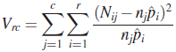
has a chi-square distribution with ![]() d.f. We reject H0 at (approximate) level α is
d.f. We reject H0 at (approximate) level α is ![]() .
.
Under the null hypothesis that the proportions of viewers who prefer the four types of programs are the same in each city, the maximum likelihood estimates of pi, ![]() are given by
are given by

Here p1 = proportion of people who prefer mystery, and so on. The following table gives the expected frequencies under H0.
| Expected Number of Responses Under H0 | ||||
| Program Type | Toledo | Columbus | Cleveland | Cincinnati |
| Mystery | 150×0.33 = 49.5 | 200×0.33 = 66 | 250×0.33 = 82.5 | 200×0.33 = 66 |
| Soap | 150×0.24 = 36 | 200×0.24 = 48 | 250×0.24 = 60 | 200×0.24 = 48 |
| Comedy | 150×0.28 = 42 | 200×0.28 = 56 | 250×0.28 = 70 | 200×0.28 = 56 |
| News | 150×0.15 = 22.5 | 200×0.15 = 30 | 250×0.15 = 37.5 | 200×0.15 = 30 |
| Sample | 150 | 200 | 250 | 200 |
| Size | ||||
It follows that

Since ![]() and
and ![]() , the number of degrees of freedom is
, the number of degrees of freedom is ![]() and we note that under H0
and we note that under H0
With such a large P-value we can hardly reject H0. The data do not offer any evidence to conclude that the proportions in the four cities are different.
PROBLEMS 10.3
- The standard deviation of capacity for batteries of a standard type is known to be 1.66 ampere-hours. The following capacities (ampere-hours) were recorded for 10 batteries of a new type: 146, 141, 135, 142, 140, 143, 138, 137, 142, 136. Does the new battery differ from the standard type with respect to variability of capacity (Natrella [75, p. 4-1])?
- A manufacturer recorded the cut-off bias (volts) of a sample of 10 tubes as follows:12.1, 12.3, 11.8, 12.0, 12.4, 12.0, 12.1, 11.9, 12.2, 12.2. The variability of cut-off bias for tubes of a standard type as measured by the standard deviation is 0.208 volts. Is the variability of the new tube, with respect to cut-off bias less than that of the standard type (Natrella [75, p. 4–5])?
- Approximately equal numbers of four different types of meters are in service and all types are believed to be equally likely to break down. The actual numbers of breakdowns reported are as follows:
Type of Meter 1 2 3 4 Number of Breakdowns Reported 30 40 33 47 Is there evidence to conclude that the chances of failure of the four types are not equal (Natrella [75, p. 9-4])?
- Every clinical thermometer is classified into one of four categories, A, B, C, D, on the basis of inspection and test. From past experience it is known that thermometers produced by a certain manufacturer are distributed among the four categories in the following proportions:
Category A B C D Proportion 0.87 0.09 0.03 0.01 A new lot of 1336 thermometers is submitted by the manufacturer for inspection and test, and the following distribution into the four categories results:
Category A B C D Number of Thermometers Reported 1188 91 47 10 Does this new lot of thermometers differ from the previous experience with regard to proportion of thermometers in each category (Natrella [75, p. 9-2])?
- A computer program is written to generate random numbers, X, uniformly in the interval 0
 . From 250 consecutive values the following data are obtained:
X-value 0–1.99 2–3.99 4–5.99 6–7.99 8–9.99 Frequency 38 55 54 41 62 Do these data offer any evidence that the program is not written properly?
- A machine working correctly cuts pieces of wire to a mean length of 10.5 cm with a standard deviation of 0.15 cm. Sixteen samples of wire were drawn at random from a production batch and measured with the following results (centimeters): 10.4, 10.6, 10.1, 10.3, 10.2, 10.9, 10.5, 10.8, 10.6, 10.5, 10.7, 10.2, 10.7, 10.3, 10.4, 10.5. Test the hypothesis that the machine is working correctly.
- An experiment consists in tossing a coin until the first head shows up. One hundred repetitions of this experiment are performed. The frequency distribution of the number of trials required for the first head is as follows:
Number of trials 1 2 3 4 5 or more Frequency 40 32 15 7 6 Can we conclude that the coin is fair?
- Fit a binomial distribution to the following data:
x 0 1 2 3 4 Frequency: 8 46 55 40 11 - Prove Theorem 1.
- Three dice are rolled independently 360 times each with the following results.
Face Value Die 1 Die 2 Die 3 1 50 62 38 2 48 55 60 3 69 61 64 4 45 54 58 5 71 78 73 6 77 50 67 Sample Size 360 360 360 Are all the dice equally loaded? That is, test the hypothesis
 ,
,  , where pi1 is the probability of getting an i with die 1, and so on.
 - Independent random samples of 250 Democrats, 150 Republicans, and 100 Independent voters were selected 1 week before a nonpartisan election for mayor of a large city. Their preference for candidates Albert, Basu, and Chatfield were recorded as follows.
Party Affiliation Preference Democrat Republican Independent Albert 160 70 90 Basu 32 45 25 Chatfield 30 23 15 Undecided 28 12 20 Sample Size 250 150 150 Are the proportions of voters in favor of Albert, Basu, and Chatfield the same within each political affiliation?
- Of 25 income tax returns audited in a small town, 10 were from low- and middle- income families and 15 from high-income families. Two of the low-income families and four of the high-income families were found to have underpaid their taxes. Are the two proportions of families who underpaid taxes the same?
- A candidate for a congressional seat checks her progress by taking a random sample of 20 voters each week. Last week, six reported to be in her favor. This week nine reported to be in her favor. Is there evidence to suggest that her campaign is working?
- Let {X11,X21,…,Xr1},…,{X1c,X2c,…,Xrc} be independent multinomial RVs with parameters (n1,p11,p21,…,pr1),…, (nc,p1c,p2c,…,prc) respectively. Let
 and
and  . Show that the GLR test for testing
  ,for
,for  ,
,  , where pj’s are unknown against all alternatives can be based on the statistic
10.4 t-TESTS
In this section we investigate one of the most frequently used types of tests in statistics, the tests based on a t-statistic. Let X1, X2,…,Xn be a random sample from ![]() (μ,σ2), and, as usual, let us write
(μ,σ2), and, as usual, let us write

The tests for usual null hypotheses about the mean can be derived using the GLR method. In the following table we summarize the results.
| Reject H0 at level α if | ||||
| H0 | H1 | σ2Known | σ2Unknown | |
| I. | ||||
| II. | ||||
| III. | ||||
Remark 1. A test based on a t-statistic is called a t-test. The t-tests in I and II are called one-tailed tests; the t-test in III, a two-tailed test.
Remark 2. If σ2 is known, tests I and II are UMP and test III is UMP unbiased. If σ2 is unknown, the t-tests are UMP unbiased and UMP invariant.
Remark 3. If n is large we may use normal tables instead of t-tables. The assumption of normality may also be dropped because of the central limit theorem. For small samples care is required in applying the proper test, since the tail probabilities under normal distribution and t-distribution differ significantly for small n (see Remark 6.4.2).
We next consider the two-sample case. Let X1, X2,…,Xm and Y1, Y2,…,Yn be independent random samples from ![]() (μ1,
(μ1, ![]() ) and
) and ![]() (μ2,
(μ2, ![]() ), respectively. Let us write
), respectively. Let us write

and

![]() is sometimes called the pooled sample variance. The following table summarizes the two sample tests comparing μ1 and μ2:
is sometimes called the pooled sample variance. The following table summarizes the two sample tests comparing μ1 and μ2:
| H0 | H1 | Reject H0 at level α if | ||
| (δ = Known Constant | ||||
| I. | 
|

| ||
| II. | 
|

| ||
| III. | 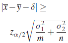
|

| ||
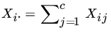
Remark 4. The case of most interest is that in which ![]() . If
. If ![]() ,
, ![]() are unknown and
are unknown and ![]() , σ2 unknown, then
, σ2 unknown, then ![]() is an unbiased estimate of σ2. In this case all the two-sample t-tests are UMP unbiased and UMP invariant. Before applying the t-test, one should first make sure that
is an unbiased estimate of σ2. In this case all the two-sample t-tests are UMP unbiased and UMP invariant. Before applying the t-test, one should first make sure that ![]() , σ2 unknown. This means applying another test on the data. We will consider this test in the next section.
, σ2 unknown. This means applying another test on the data. We will consider this test in the next section.
Remark 5. If ![]() is large, we use normal tables; if both m and n are large, we can drop the assumption of normality, using the CLT.
is large, we use normal tables; if both m and n are large, we can drop the assumption of normality, using the CLT.
Remark 6. The problem of equality of means in sampling from several populations will be considered in Chapter 12.
Remark 7. The two sample problem when ![]() , both unknown, is commonly referred to as Behrens-Fisher problem. The Welch approximate t-test of
, both unknown, is commonly referred to as Behrens-Fisher problem. The Welch approximate t-test of ![]() is based on a random number of d.f. f given by
is based on a random number of d.f. f given by

where

and the t-statistic

with f d.f. This approximation has been found to be quite good even for small samples. The formula for f generally leads to noninteger d.f. Linear interpolation in t-table can be used to obtain the required percentiles for f d.f.
Quite frequently one samples from a bivariate normal population with means μ1,μ2, variances ![]() ,
, ![]() , and correlation coefficient ρ, the hypothesis of interest being
, and correlation coefficient ρ, the hypothesis of interest being ![]() . Let (X1; Y1), (X2, Y2),…, (Xn, Yn) be a sample from a bivariate normal distribution with parameters μ1, μ2,
. Let (X1; Y1), (X2, Y2),…, (Xn, Yn) be a sample from a bivariate normal distribution with parameters μ1, μ2, ![]() ,
, ![]() , and ρ. Then Xj – Yj is
, and ρ. Then Xj – Yj is ![]() , where
, where ![]() . We can therefore treat
. We can therefore treat ![]() ,
, ![]() , as a sample from a normal population. Let us write
, as a sample from a normal population. Let us write

The following table summarizes the resulting tests:
| H0 | H1 | ||
| d0 = Known Constant | Reject H0 at level α if | ||
| I. | |||
| II. | |||
| III. | |||
Remark 8. The case of most importance is that in which ![]() . All the t-tests, based on Dj’s, are UMP unbiased and UMP invariant. If σ is known, one can base the test on a standardized normal RV, but in practice such an assumption is quite unrealistic. If n is large one can replace t-values by the corresponding critical values under the normal distribution.
. All the t-tests, based on Dj’s, are UMP unbiased and UMP invariant. If σ is known, one can base the test on a standardized normal RV, but in practice such an assumption is quite unrealistic. If n is large one can replace t-values by the corresponding critical values under the normal distribution.
Remark 9. Clearly, it is not necessary to assume that (X1, Y1),…,(Xn, Yn) is a sample from a bivariate normal population. It suffices to assume that the differences Di form a sample from a normal population.
PROBLEMS 10.4
- The manufacturer of a certain subcompact car claims that the average mileage of this model is 30 miles per gallon of regular gasoline. For nine cars of this model driven in an identical manner, using 1 gallon of regular gasoline, the mean distance traveled was 26 miles with a standard deviation of 2.8 miles. Test the manufacturer’s claim if you are willing to reject a true claim no more than twice in 100.
- The nicotine contents of five cigarettes of a certain brand showed a mean of 21.2 milligrams with a standard deviation of 2.05 milligrams. Test the hypothesis that the average nicotine content of this brand of cigarettes does not exceed 19.7 milligrams. Use
 .
. - The additional hours of sleep gained by eight patients in an experiment with a certain drug were recorded as follows:
Patient 1 2 3 4 5 6 7 8 Hours Gained 0.7 −1.1 3.4 0.8 2.0 0.1 −0.2 3.0 Assuming that these patients form a random sample from a population of such patients and that the number of additional hours gained from the drug is a normal random variable, test the hypothesis that the drug has no effect at level
 .
. - The mean life of a sample of 8 light bulbs was found to be 1432 hours with a standard deviation of 436 hours. A second sample of 19 bulbs chosen from a different batch produced a mean life of 1310 hours with a standard deviation of 382 hours. Making appropriate assumptions, test the hypothesis that the two samples came from the same population of light bulbs at level
 .
. - A sample of 25 observations has a mean of 57.6 and a variance of 1.8. A further sample of 20 values has a mean of 55.4 and a variance of 2.5. Test the hypothesis that the two samples came from the same normal population.
- Two methods were used in a study of the latent heat of fusion of ice. Both method A and method B were conducted with the specimens cooled to −0.72°C. The following data represent the change in total heat from −0.72°C to water, 0°C, in calories per gram of mass:
- Method A: 79.98,80.04,80.02,80.04,80.03,80.03,80.04,79.97,80.05,80.03, 80.02,80.00,80.02
- Method B: 80.02,79.74,79.98,79.97,79.97,80.03,79.95,79.97
Perform a test at level 0.05 to see whether the two methods differ with regard to their average performance (Natrella [75, p. 3-23]).
- In Problem 6, if it is known from past experience that the standard deviations of the two methods are
 and
and  , test the hypothesis that the methods are same with regard to their average performance at level
  .
. - During World War II bacterial polysaccharides were investigated as blood plasma extenders. Sixteen samples of hydrolyzed polysaccharides supplied by various manufacturers in order to assess two chemical methods for determining the average molecular weight yielded the following results:
- Method A: 62,700; 29,100; 44,400; 47,800; 36,300; 40,000; 43,400; 35,800; 33,900; 44,200; 34,300; 31,300; 38,400; 47,100; 42,100; 42,200
- Method B: 56,400; 27,500; 42,200; 46,800; 33,300; 37,100; 37,300; 36,200; 35,200; 38,000; 32,200; 27,300; 36,100; 43,100; 38,400; 39,900
Perform an appropriate test of the hypothesis that the two averages are the same against a one-sided alternative that the average of Method A exceeds that of Method B. Use
 . (Natrella [75, p. 3-38]).
 - The following grade-point averages were collected over a period of 7 years to determine whether membership in a fraternity is beneficial or detrimental to grades:
Year 1 2 3 4 5 6 7 FraternityFraternity 2.4 2.0 2.3 2.1 2.1 2.0 2.0 Nonfraternity 2.4 2.2 2.5 2.4 2.3 1.8 1.9 Assuming that the populations were normal, test at the 0.025 level of significance whether membership in a fraternity is detrimental to grades.
- Consider the two sample t-statistic
 , where
  . Suppose
  . Let m, n → ∞ such that
  . Show that, under
  , , where
  , where
  . Thus when
  and
and  and T is approximately
  (0,1) as
  . In this case, a t-test based on T will have approximately the right level.
10.5 F-TESTS
The term F-tests refers to tests based on an F-statistic. Let X1,X2,…,Xm and Y1,Y2,…,Yn be independent samples from ![]() and
and ![]() , respectively. We recall that
, respectively. We recall that ![]() and
and ![]() are independent RVs, so that the RV
are independent RVs, so that the RV

is distributed as ![]() .
.
The following table summarizes the F-tests:
| Reject H0 at level α if | ||||
| H0 | H1 | μ1, μ2 Known | μ1, μ2 Unknown | |
| I. | 
|
|||
| II. | 
|
| ||
| III. | 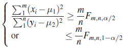
|

| ||
Remark 1. Recall (Remark 6.4.5) that
Remark 2. The tests described above can be easily obtained from the likelihood ratio procedure. Moreover, in the important case where μ1, μ2 are unknown, tests I and II are UMP unbiased and UMP invariant. For test III we have chosen equal tails, as is customarily done for convenience even though the unbiasedness property of the test is thereby destroyed.
An important application of the F-test involves the case where one is testing the equality of means of two normal populations under the assumption that the variances are the same, that is, testing whether the two samples come from the same population. Let X1, X2, …,Xm and Y1, Y2, …,Yn be independent samples from ![]() and
and ![]() , respectively. If
, respectively. If ![]() but is unknown, the t-test rejects
but is unknown, the t-test rejects ![]() if
if ![]() , where c is selected so that
, where c is selected so that ![]() , that is,
, that is, ![]() , where
, where

s1, s2 being the sample variances. If first an F-test is performed to test ![]() , and then a t-test to test
, and then a t-test to test ![]() at levels α1 and α2, respectively, the probability of accepting both hypotheses when they are true is
at levels α1 and α2, respectively, the probability of accepting both hypotheses when they are true is
and if F is independent of T, this probability is (1–α1)(1–α2). It follows that the combined test has a significance level ![]() . We see that
. We see that
and ![]() . In fact, α will be closer to
. In fact, α will be closer to ![]() , since for small α1 and α2, α1α2 will be closer to 0.
, since for small α1 and α2, α1α2 will be closer to 0.
We show that F is independent of T whenever ![]() . The statistic
. The statistic  is a complete sufficient statistic for the parameter
 ![]() (see Theorem 8.3.2). Since the distribution of F does not depend on μ1, μ2, and
(see Theorem 8.3.2). Since the distribution of F does not depend on μ1, μ2, and ![]() , it follows (Problem 5) that F is independent of V whenever
, it follows (Problem 5) that F is independent of V whenever ![]() . But T is a function of V alone, so that F must be independent of T also.
. But T is a function of V alone, so that F must be independent of T also.
In Example 1, the combined test has a significance level of
PROBLEMS 10.5
- For the data of Problem 10.4.4 is the assumption of equality of variances, on which the t-test is based, valid?
- Answer the same question for Problems 10.4.5 and 10.4.6.
- The performance of each of two different dive bombing methods is measured a dozen times. The sample variances for the two methods are computed to be 5545 and 4073, respectively. Do the two methods differ in variability?
- In Problem 3 does the variability of the first method exceed that of the second method?
- Let X = (X1, X2,…,Xn) be a random sample from a distribution with PDF (PMF) f (x, θ),
 where Θ is an interval in
  . Let T (X) be a complete sufficient statistic for the family {f (x; θ):
  }. If U(X) is a statistic (not a function of T alone) whose distribution does not depend on θ, show that U is independent of T.
10.6 BAYES AND MINIMAX PROCEDURES
Let X1, X2,…,Xn be a sample from a probability distribution with PDF (PMF) fθ, ![]() . In Section 8.8 we described the general decision problem, namely, once the statistician observes x, she has a set
. In Section 8.8 we described the general decision problem, namely, once the statistician observes x, she has a set ![]() of options available. The problem is to find a decision function d that minimizes the risk
of options available. The problem is to find a decision function d that minimizes the risk ![]() in some sense. Thus a minimax solution requires the minimization of max R(θ, δ) , while a Bayes solution requires the minimization of
in some sense. Thus a minimax solution requires the minimization of max R(θ, δ) , while a Bayes solution requires the minimization of ![]() , where π is the a priori distribution on Θ. In Remark 9.2.1 we considered the problem of hypothesis testing as a special case of the general decision problem. The set
, where π is the a priori distribution on Θ. In Remark 9.2.1 we considered the problem of hypothesis testing as a special case of the general decision problem. The set ![]() contains two points, a0 and a1; a0 corresponds to the acceptance of
contains two points, a0 and a1; a0 corresponds to the acceptance of ![]() , and a1 corresponds to the rejection of H0. Suppose that the loss function is defined by
, and a1 corresponds to the rejection of H0. Suppose that the loss function is defined by

Then

A minimax solution to the problem of testing ![]() against
against ![]() , where
, where ![]() , is to find a rule δ that minimizes
, is to find a rule δ that minimizes
We will consider here only the special case of testing ![]() against
against ![]() . In that case we want to find a rule δ which minimizes
. In that case we want to find a rule δ which minimizes
We will show that the solution is to reject H0 if

provided that the constant k is chosen so that
where δ is the rule defined in (5); that is, the minimax rule δ is obtained if we choose k in (5) so that
or, equivalently, we choose k so that

Let δ* be any other rule. If ![]() , then
, then ![]() and δ* cannot be minimax. Thus,
and δ* cannot be minimax. Thus, ![]() , which means that
, which means that
By the Neyman-Pearson lemma, rule δ is the most powerful of its size, so that its power must be at least that of δ*, that is,
so that
It follows that
and hence that
This means that
and thus
Note that in the discrete case one may need some randomization procedure in order to achieve equality in (8).
We next consider the problem of testing ![]() against
against ![]() from a Bayesian point of view. Let π(θ) be the a priori probability distribution on Θ.
from a Bayesian point of view. Let π(θ) be the a priori probability distribution on Θ.
Then

The Bayes solution is a decision rule that minimizes R(π, δ). In what follows we restrict our attention to the case where both H0 and H1 have exactly one point each, that is, ![]() ,
, ![]() . Let
. Let ![]() and
and ![]() . Then
. Then
where ![]() ,
, ![]() .
.
The a posteriori distribution of θ is given by


Thus

It follows that we reject H0, that is, ![]() if
if
which is the case if and only if
as asserted.
Remark 1. In the Neyman-Pearson lemma we fixed ![]() , the probability of rejectingH0 when it is true, and minimized
, the probability of rejectingH0 when it is true, and minimized ![]() , the probability of accepting H0 when it is false. Here we no longer have a fixed level α for
, the probability of accepting H0 when it is false. Here we no longer have a fixed level α for ![]() . Instead we allow it to assume any value as long as R(π, δ), defined in (12), is minimum.
. Instead we allow it to assume any value as long as R(π, δ), defined in (12), is minimum.
Remark 2. It is easy to generalize Theorem 1 to the case of multiple decisions. Let X be an RV with PDF (PMF) fθ , where θ can take any of the k values θ1 , θ2,…, θk . The problem is to observe x and decide which of the θi’ is the correct value of θ. Let us write ![]() ,
, ![]() , and assume that
, and assume that ![]() ,
, ![]() ,
, ![]() , is the prior probability distribution on
, is the prior probability distribution on ![]() . Let
. Let

The problem is to find a rule δ that minimizes R(π ,δ). We leave the reader to show that a Bayes solution is to accept ![]() if
if
where any point lying in more than one such region is assigned to any one of them.
PROBLEMS 10.6
- In Example 1 let
 ,
,  , and
, and  , and choose
  . Find the minimax test, and compute its power at
  and
and  .
. - A sample of five observations is taken on a b(1 ,θ) RV to test H0:
 against
  .
.- Find the most powerful test of size
 .
. - If
 ,
,  , and
, and  , find the minimax rule.
 - If the prior probabilities of
 and
and  are
are  and
and  , respectively, find the Bayes rule.
- Find the most powerful test of size
- A sample of size n is to be used from the PDF

to test
 against
  . If the a priori distribution on θ is
  ,
,  , and
, and  , find the Bayes solution. Find the power of the test at
  and
and  .
. - Given two normal densities with variances 1 and with means –1 and 1, respectively, find the Bayes solution based on a single observation when
 and (a)
  , and (b)
  ,
,  .
. - Given three normal densities with variances 1 and with means –1, 0, 1, respectively, find the Bayes solution to the multiple decision problem based on a single observation when
 ,
,  ,
,  .
. - For the multiple decision problem described in Remark 2 show that a Bayes solution is to accept
 if (15) holds.