12
GENERAL LINEAR HYPOTHESIS
12.1 INTRODUCTION
This chapter deals with the general linear hypothesis. In a wide variety of problems the experimenter is interested in making inferences about a vector parameter. For example, he may wish to estimate the mean of a multivariate normal or to test some hypotheses concerning the mean vector. The problem of estimation can be solved, for example, by resorting to the method of maximum likelihood estimation, discussed in Section 8.7. In this chapter we restrict ourselves to the so-called linear model problems and concern ourselves mainly with problems of hypotheses testing.
In Section 12.2 we formally describe the general model and derive a test in complete generality. In the next four sections we demonstrate the power of this test by solving four important testing problems. We will need a considerable amount of linear algebra in Section 12.2.
12.2 GENERAL LINEAR HYPOTHESIS
A wide variety of problems of hypotheses testing can be treated under a general setup. In this section we state the general problem and derive the test statistic and its distribution. Consider the following examples.
where t is a mathematical variable, β 0, β1, β2 are unknown parameters, and ε is a nonobservable RV. The experimenter takes observations Y1,Y2,…,Yn at predetermined values t1,t2,…,tn, respectively, and is interested in testing the hypothesis that the relation is in fact linear, that is, ![]() .
.
Examples of the type discussed above and their much more complicated variants can all be treated under a general setup. To fix ideas, let us first make the following definition.
In what follows we will assume that ε1,2,…,εn are independent, normal RVs with common variance σ2 and ![]() ,
, ![]() . In view of (2), it follows that Y1,Y2,…,Yn are independent normal RVs with
. In view of (2), it follows that Y1,Y2,…,Yn are independent normal RVs with

We will assume that H is a matrix of full rank r, ![]() , and X is a matrix of full rank
, and X is a matrix of full rank ![]() . Some remarks are in order.
. Some remarks are in order.
Remark 1. Clearly, Y satisfies a linear model if the vector of means ![]() lies in a k-dimensional subspace generated by the linearly independent column vectors x1,x2,…,xk of the matrix X. Indeed, (1) states that EY is a linear combination of the known vectors x1,…,xk. The general linear hypothesis
lies in a k-dimensional subspace generated by the linearly independent column vectors x1,x2,…,xk of the matrix X. Indeed, (1) states that EY is a linear combination of the known vectors x1,…,xk. The general linear hypothesis ![]() states that the parameters β1,β2,…,βk satisfy r independent homogeneous linear restrictions. It follows that, under H0, EY lies in a
states that the parameters β1,β2,…,βk satisfy r independent homogeneous linear restrictions. It follows that, under H0, EY lies in a ![]() -dimensional subspace of the k-space generated by x1,…,xk.
-dimensional subspace of the k-space generated by x1,…,xk.
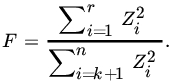
Remark 2. The assumption of normality, which is conventional, is made to compute the likelihood ratio test statistic of H0 and its distribution. If the problem is to estimate β, no such assumption is needed. One can use the principle of least squares and estimate β by minimizing the sum of squares,

The minimizing value ![]() is known as a least square estimate of β. This is not a difficult problem, and we will not discuss it here in any detail but will mention only that any solution of the so-called normal equations
is known as a least square estimate of β. This is not a difficult problem, and we will not discuss it here in any detail but will mention only that any solution of the so-called normal equations
is a least square estimator. If the rank of X is ![]() , then X' X, which has the same rank as X, is a nonsingular matrix that can be inverted to give a unique least square estimator
, then X' X, which has the same rank as X, is a nonsingular matrix that can be inverted to give a unique least square estimator
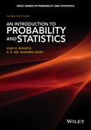
If the rank of X is ![]() , then X' X is singular and the normal equations do not have a unique solution. One can show, for example, that
, then X' X is singular and the normal equations do not have a unique solution. One can show, for example, that ![]() is unbiased for β, and if the Yi’s are uncorrelated with common variance σ2, the variance-covariance matrix of the
is unbiased for β, and if the Yi’s are uncorrelated with common variance σ2, the variance-covariance matrix of the ![]() ’s is given by
’s is given by
Remark 3. One can similarly compute the so-called restricted least square estimator of β by the usual method of Lagrange multipliers. For example, under ![]() one simply minimizes
one simply minimizes ![]() subject to
subject to ![]() to get the restricted least square estimator
to get the restricted least square estimator ![]() . The important point is that, if ε is assumed to be a multivariate normal RV with mean vector 0 and dispersion matrix σ2In, the MLE of β is the same as the least square estimator. In fact, one can show that
. The important point is that, if ε is assumed to be a multivariate normal RV with mean vector 0 and dispersion matrix σ2In, the MLE of β is the same as the least square estimator. In fact, one can show that ![]() is the UMVUE of
is the UMVUE of ![]() , by the usual methods.
, by the usual methods.
Similarly, we may assume that the regression of Y on x is quadratic:
and we may wish to test that a linear function will be sufficient to describe the relationship, that is, ![]() . Here X is the
. Here X is the ![]() matrix
matrix

and H is the ![]() matrix (0, 0, 1).
matrix (0, 0, 1).
In another example of regression, the Y's can be written as
and we wish to test the hypothesis that ![]() . In this case, X is the matrix
. In this case, X is the matrix

and H may be chosen to be the ![]() matrix
matrix

The model described in this example is frequently referred to as a one-way analysis of variance model. This is a very simple example of an analysis of variance model. Note that the matrix X is of a very special type, namely, the elements of X are either 0 or 1. X is known as a design matrix.
Returning to our general model
we wish to test the null hypothesis ![]() . We will compute the likelihood ratio test and the distribution of the test statistic. In order to do so, we assume that ε has a multivariate normal distribution with mean vector 0 and variance-covariance matrix σ2in, where σ2 is unknown and In is the
. We will compute the likelihood ratio test and the distribution of the test statistic. In order to do so, we assume that ε has a multivariate normal distribution with mean vector 0 and variance-covariance matrix σ2in, where σ2 is unknown and In is the ![]() identity matrix. This means that Y has an n-variate normal distribution with mean Xβ and dispersion matrix σ2In for some β and some σ2, both unknown. Here the parameter space Θ is the set of
identity matrix. This means that Y has an n-variate normal distribution with mean Xβ and dispersion matrix σ2In for some β and some σ2, both unknown. Here the parameter space Θ is the set of ![]() -tuples
-tuples ![]() , and the joint PDF of the X's is given by
, and the joint PDF of the X's is given by

It remains to determine the distribution of the test statistic. For this purpose it is convenient to reduce the problem to the canonical form. Let Vn be the vector space of the observation vector Y, Vk be the subspace of Vn generated by the column vectors x1, x2,…,xk of X, and ![]() be the subspace of Vk in which EY is postulated to lie under H0. We change variables from Y1,Y2,…,Yn to Z1,Z2,…,Zn, where Z1,Z2,…,Zn are independent normal RVs with common variance σ2 and means
be the subspace of Vk in which EY is postulated to lie under H0. We change variables from Y1,Y2,…,Yn to Z1,Z2,…,Zn, where Z1,Z2,…,Zn are independent normal RVs with common variance σ2 and means ![]() ,
, ![]() . This is done as follows. Let us choose an orthonormal basis of
. This is done as follows. Let us choose an orthonormal basis of ![]() column vectors {ai} for
column vectors {ai} for ![]() , say
, say ![]() . We extend this to an orthonormal basis
. We extend this to an orthonormal basis ![]() for Vk, and then extend once again to an orthonormal basis
for Vk, and then extend once again to an orthonormal basis ![]() for Vn. This is always possible.
for Vn. This is always possible.
Let z1, z2,…,zn be the coordinates of y relative to the basis {α1, α2, …, αn}. Then ![]() and
and ![]() , where P is an orthogonal matrix with ith row
, where P is an orthogonal matrix with ith row ![]() . Thus
. Thus ![]() , and
, and ![]() . Since Xβ ∈ Vk (Remark 1), it follows that
. Since Xβ ∈ Vk (Remark 1), it follows that ![]() for
for ![]() . Similarly, under H0,
. Similarly, under H0, ![]() , so that
, so that ![]() for
for ![]() . Let us write
. Let us write ![]() . Then
. Then ![]() , and under
, and under ![]() . Finally, from Corollary 2 of Theorem 6 it follows that Z1, Z2,…,Zn are independent normal RVs with the same variance σ2 and
. Finally, from Corollary 2 of Theorem 6 it follows that Z1, Z2,…,Zn are independent normal RVs with the same variance σ2 and ![]() . We have thus transformed the problem to the following simpler canonical form:
. We have thus transformed the problem to the following simpler canonical form:

Now

The quantity ![]() is minimized if we choose
is minimized if we choose ![]() , so that
, so that

Under ![]() , so that
, so that ![]() will be minimized if we choose
will be minimized if we choose ![]() . Thus
. Thus

It follows that
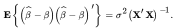
Now ![]() has a
has a ![]() distribution, and, under
distribution, and, under ![]() has a χ2(r) distribution. Since
has a χ2(r) distribution. Since ![]() and
and ![]() are independent, we see that
are independent, we see that ![]() is distributed as
is distributed as ![]() under H0, as asserted. This completes the proof of the theorem.
under H0, as asserted. This completes the proof of the theorem.
Remark 4. In practice, one does not need to find a transformation that reduces the problem to the canonical form. As will be done in the following sections, one simply computes the estimators ![]() and
and ![]() and then computes the test statistic in any of the equivalent forms (14), (15), or (16) to apply the F-test.
and then computes the test statistic in any of the equivalent forms (14), (15), or (16) to apply the F-test.
Remark 5. The computation of ![]() is greatly facilitated, in view of Remark 3, by using the principle of least squares. Indeed, this was done in the proof of Theorem 1 when we reduced the problem of maximum likelihood estimation to that of minimization of sum of squares
is greatly facilitated, in view of Remark 3, by using the principle of least squares. Indeed, this was done in the proof of Theorem 1 when we reduced the problem of maximum likelihood estimation to that of minimization of sum of squares ![]() .
.
Remark 6. The distribution of the test statistic under H1 is easily determined. We note that ![]() for
for ![]() , so that
, so that ![]() has a noncentral chi-square distribution with r d.f. and noncentrality parameter
has a noncentral chi-square distribution with r d.f. and noncentrality parameter ![]() . It follows that
. It follows that ![]() has a noncentral F-distribution with d.f.
has a noncentral F-distribution with d.f. ![]() and noncentrality parameter δ. Under
and noncentrality parameter δ. Under ![]() , so that
, so that ![]() has a central
has a central ![]() distribution. Since
distribution. Since ![]() , it follows from (19) and (20) that if we replace each observation Yi bu its expected value in the numerator of (16), we get σ2δ.
, it follows from (19) and (20) that if we replace each observation Yi bu its expected value in the numerator of (16), we get σ2δ.
Remark 7. The general linear hypothesis makes use of the assumption of common variance. For instance, in Example 4, ![]() . Let us suppose that
. Let us suppose that ![]() .. Then we need to test that
.. Then we need to test that ![]() before we can apply Theorem 1. The case
before we can apply Theorem 1. The case ![]() has already been considered in Section 10.3. For the case where
has already been considered in Section 10.3. For the case where ![]() one can show that a UMP unbiased test does not exist. A large-sample approximation is described in Lehmann [64, pp. 376–377]. It is beyond the scope of this book to consider the effects of departures from the underlying assumptions. We refer the reader to Scheffé [101, Chapter 10], for a discussion of this topic.
one can show that a UMP unbiased test does not exist. A large-sample approximation is described in Lehmann [64, pp. 376–377]. It is beyond the scope of this book to consider the effects of departures from the underlying assumptions. We refer the reader to Scheffé [101, Chapter 10], for a discussion of this topic.
Remark 8. The general linear model (GLM) is widely used in social sciences where Y is often referred to as the response (or dependent) variable and X as the explanatory (or independent) variable. In this language the GLM “predicts” a response variable from a linear combination of one or more explanatory variables. It should be noted that dependent and independent in this context do not have the same meaning as in Chapter 4. Moreover, dependence does not imply causality.
PROBLEMS 12.2
- Show that any solution of the normal equations (5) minimizes the sum of squares
 .
. - Show that the least square estimator given in (6) is an unbiased estimator of β. If the RVs Yi are uncorrelated with common variance σ2, show that the covariance matrix of the
 ’s is given by (7).
 - Under the assumption that ε [in model (2)] has a multivariate normal distribution with mean 0 and dispersion matrix σ2In show that the least square estimators and the MLE's of β coincide.
- Prove statements (11) and (12).
- Determine the expression for the least squares estimator of β subject to

12.3 REGRESSION ANALYSIS
In this section we study regression analysis, which is a tool to investigate the interrelationship between two or more variables. Typically, in its simplest form a response random variable Y is hypothesized to be related to one or more explanatory nonrandom variables xi's. Regression analysis with a single explanatory RV is known as simple regression and if, in addition, the relationship is thought to be linear, it is called simple linear regression (Example 12.2.3). In the case where several explanatory variables xi's are involved the regression is referred to as multiple linear regression. Regression analysis is widely used in forecasting and prediction. Again this is a special case of GLM.
This section is divided into three subsections. The first subsection deals with multiple linear regression where the RV Y is of the continuous type. In the next two subsections we study the case when Y is either Bernoulli or a count variable.
12.3.1 Multiple Linear Regression
It is convenient to write GLM in the form
where Y,X,ε, and β are as in Equation (12.2.1), and 1n is the column ![]() unit vector (1,1,…, 1). The parameter β0 is usually referred to as the intercept whereas β is known as the slope vector with k parameters. The least estimator (LSE) of β0 and β are easily obtained by minimizing.
unit vector (1,1,…, 1). The parameter β0 is usually referred to as the intercept whereas β is known as the slope vector with k parameters. The least estimator (LSE) of β0 and β are easily obtained by minimizing.

resulting in ![]() normal equations
normal equations

or

and

An unbiased estimate of σ2 is given by
Let us now consider the simple linear regression model
The LSEs of (β0, β)′ is given by

and

The covariance matrix is given by

where ![]()
Let us now verify these results using the maximum likelihood method.
Clearly, Y1,Y2,…,Yn are independent normal RVs with ![]() and
and ![]() , and Y is an n-variate normal random vector with mean Xβ and variance σ2In. The joint PDF of Y is given by
, and Y is an n-variate normal random vector with mean Xβ and variance σ2In. The joint PDF of Y is given by

It easily follows that the MLE’s for β0, β1 and σ2 are given by


and

where ![]() .
.
If we wish to test ![]() , we take
, we take ![]() , so that the model is a special case of the general linear hypothesis with
, so that the model is a special case of the general linear hypothesis with ![]() ,
, ![]() . Under H0 the MLE’s are
. Under H0 the MLE’s are

and

Thus

From Theorem 12.2.1, the statistic ![]() has a central
has a central ![]() distribution under H0. Since
distribution under H0. Since ![]() is the square of a
is the square of a ![]() , the likelihood ratio test rejects H0 if
, the likelihood ratio test rejects H0 if

where c0 is computed from t-tables for ![]() d.f.
d.f.
For testing ![]() , we choose
, we choose ![]() so that the model is again a special case of the general linear hypothesis. In this case
so that the model is again a special case of the general linear hypothesis. In this case

and

It follows that

and since

we can write the numerator of F as

It follows from Theorem 12.2.1 that the statistic

has a central t-distribution with ![]() d.f. under
d.f. under ![]() . The rejection region is therefore given by
. The rejection region is therefore given by

where c0 is determined from the tables of ![]() distribution for a given level of significance α.
distribution for a given level of significance α.
For testing ![]() , we choose
, we choose  , so that the model is again a special case of the general linear hypothesis with
 ![]() . In this case
. In this case

and

From Theorem 12.2.1, the statistic ![]() has a central
has a central ![]() distribution under
distribution under ![]() . It follows that the α-level rejection region for H0 is given by
. It follows that the α-level rejection region for H0 is given by
where F is given by (26), and c0 is the upper α percent point under the ![]() distribution.
distribution.
Remark 1. It is quite easy to modify the analysis above to obtain tests of null hypotheses ![]() , and
, and ![]() , where
, where ![]() are given real numbers (Problem 4).
are given real numbers (Problem 4).
Remark 2.. The confidence intervals for β0, β1 are also easily obtained. One can show that ![]() -level confidence interval for β0 is given by
-level confidence interval for β0 is given by

and that for β1 is given by

Similarly, one can obtain confidence sets for (β0, β1)′ from the likelihood ratio test of ![]() . It can be shown that the collection of sets of points (β0, β1)′ satisfying
. It can be shown that the collection of sets of points (β0, β1)′ satisfying

is a ![]() -level collection of confidence sets (ellipsoids) for (β0, β1)′ centered at
-level collection of confidence sets (ellipsoids) for (β0, β1)′ centered at ![]() .
.
Remark 3. Sometimes interest lies in constructing a confidence interval on the unknown linear regression function ![]() for a given value of x, or on a value of Y, given
for a given value of x, or on a value of Y, given ![]() . We assume that x0 is a value of x distinct from x1,x2,…,xn. Clearly,
. We assume that x0 is a value of x distinct from x1,x2,…,xn. Clearly, ![]() is the maximum likelihood estimator of
is the maximum likelihood estimator of ![]() . This is also the best linear unbiased estimator. Let us write
. This is also the best linear unbiased estimator. Let us write ![]() . Then
. Then

which is clearly a linear function of normal RVs Yi. It follows that ![]() is also normally distributed with mean
is also normally distributed with mean ![]() and variance
and variance

(See Problem 6.) It follows that

is ![]() (0,1). But σ is not known, so that we cannot use (32) to construct a confidence interval for
(0,1). But σ is not known, so that we cannot use (32) to construct a confidence interval for ![]() . Since
. Since ![]() is a
is a ![]() RV and
RV and ![]() is independent of
is independent of ![]() (why?), it follows that
(why?), it follows that

has a ![]() distribution. Thus, a
distribution. Thus, a ![]() -level confidence interval for
-level confidence interval for ![]() is given by
is given by

In a similar manner one can show (Problem 7) that

is a ![]() -level confidence interval for
-level confidence interval for ![]() , that is, for the estimated value Y0 of Y at x0.
, that is, for the estimated value Y0 of Y at x0.
Remark 4. The simple regression model (2) considered above can be generalized in many directions. Thus we may consider EY as a polynomial in x of a degree higher than 1, or we may regard EY as a function of several variables. Some of these generalizations will be taken up in the problems.
Remark 5. Let (X1, Y1), (X2, Y2),…,(Xn, Yn) be a sample from a bivariate normal population with parameters ![]() ,
,![]() ,
,![]() ,
,![]() , and
, and ![]() .
.
In Section 6.6 we computed the PDF of the sample correlation coefficient R and showed (Remark 6.6.4) that the statistic

has a ![]() distribution, provided that
distribution, provided that ![]() . If we wish to test
. If we wish to test ![]() , that is, the independence of two jointly normal RVs, we can base a test on the statistic T. Essentially, we are testing that the population covariance is 0, which implies that the population regression coefficients are 0. Thus we are testing, in particular, that
, that is, the independence of two jointly normal RVs, we can base a test on the statistic T. Essentially, we are testing that the population covariance is 0, which implies that the population regression coefficients are 0. Thus we are testing, in particular, that ![]() . It is therefore not surprising that (36) is identical with (18). We emphasize that we derived (36) for a bivariate normal population, but (18) was derived by taking the X’s as fixed and the distribution of Y’s as normal. Note that for a bivariate normal population
. It is therefore not surprising that (36) is identical with (18). We emphasize that we derived (36) for a bivariate normal population, but (18) was derived by taking the X’s as fixed and the distribution of Y’s as normal. Note that for a bivariate normal population ![]() is linear, in consistency with our model (1) or (2).
is linear, in consistency with our model (1) or (2).
Let us next find a 95 percent confidence interval for ![]() . This is given by (34). We have
. This is given by (34). We have


so that the 95 percent confidence interval is ![]() .
.
(The data were produced from Table ST6, of random numbers with ![]() , by letting
, by letting ![]() and
and ![]() so that
so that ![]() , which surely lies in the interval.)
, which surely lies in the interval.)
12.3.2 Logistic and Poisson Regression
In the regression model considered above Y is a continuous type RV. However, in a wide variety of problems Y is either binary or a count variable. Thus in a medical study Y may be the presence or absence of a disease such as diabetes. How do we modify linear regression model to apply in this case? The idea here is to choose a function of E(Y) so that in Section 12.3.1
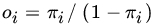
This can be accomplished by choosing the function f to be the logarithm of the odds ratio

where ![]() so that
so that ![]() . It follows that
. It follows that

so that logistic regression models the logarithm of odds ratio as a linear function of RVs Xi. The term logistic regression derives from the fact that the function ![]() is known as the logistic function.
is known as the logistic function.
For simplicity we will only consider the simple linear regression model case so that
Choosing the logistic distribution as

let Y1, Y2,…,Yn be iid binary RVs taking values 0 or 1. Then the joint PMF of Y1, Y2,…,Yn is given by

and the log likelihood function by

It is easy to see that

Since the likelihood equations are nonlinear in the parameters, the MLEs of β0 and β are obtained numerically by using Newton-Raphson method.
Let ![]() and
and ![]() be the MLE of β0 and β, respectively. From section 8.7 we note that the variance of
be the MLE of β0 and β, respectively. From section 8.7 we note that the variance of ![]() is given by
is given by

so that the standard error (SE) of ![]() is its square root. For large n, the so-called Wald statistic
is its square root. For large n, the so-called Wald statistic ![]() has an approximate N(0, 1) distribution under
has an approximate N(0, 1) distribution under ![]() . Thus we reject H0 at level α if
. Thus we reject H0 at level α if ![]() . One can use
. One can use ![]() as a (1–α) -level confidence interval for β.
as a (1–α) -level confidence interval for β.
Yet another choice for testing H0 is to use the LRT statistics –2logλ (see Theorem 10.2.3). Under H0, ![]() has a chi-square distribution with 1 d.f. Here
has a chi-square distribution with 1 d.f. Here

In (40) we chose the DF of a logistic RV. We could have chosen some other DF such as ϕ(x), the DF of a N(0, 1) RV. In that case we have ![]() . The resulting model is called probit regression.
. The resulting model is called probit regression.
We finally consider the case when the RV Y is a count of rare events and has Poisson distribution with parameter λ. Clearly, the GLM is not directly applicable. Again we only consider the linear regression model case. Let ![]() , be independent P(λi)RVs where
, be independent P(λi)RVs where ![]() , so that
, so that
The log likelihood function is given by

In order to find the MLEs of β0 and β1 we need to solve the likelihood equations

which are nonlinear in β0 and β1. The most common method of obtaining the MLEs is to apply the iteratively weighted least squares algorithm.
Once the MLEs of β0 and β1 are computed, one can compute the SEs of the estimates by using methods of Section 8.7. Using the SE ![]() , for example, one can test hypothesis concerning β1 or construct
, for example, one can test hypothesis concerning β1 or construct ![]() -level confidence interval for β1.
-level confidence interval for β1.
For a detailed discussion of Geometric and Poisson regression we refer Agresti [1] . A wide variety of software is available, which can be used to carry out the computations required.
PROBLEMS 12.3
- Prove statements (12), (13), and (14).
- Prove statements (15) and (16).
- Prove statement (19).
- Obtain tests of null hypotheses
 , and
, and  , where
  are given real numbers.
 - Obtain the confidence intervals for β0 and β1 as given in (28) and (29), respectively.
- Derive the expression for
 as given in (31).
 - Show that the interval given in (35) is a (1—α) -level confidence interval for
 , the estimated value of Y at x0.
 - Suppose that the regression of Y on the (mathematical) variable x is a quadratic

where β0, β1, β2 are unknown parameters, x1, x2,…,xn are known values of x, and ε1, ε2,…,εn are unobservable RVs that are assumed to be independently normally distributed with common mean 0 and common variance σ2 (see Example 12.2.3). Assume that the coefficient vectors
 , are linearly independent. Write the normal equations for estimating the β's and derive the generalized likelihood ratio test of
  .
. - Suppose that the Y's can be written as

where xi1, xi2, xi3 are three mathematical variables, and εi are iid
 (0,1) RVs. Assuming that the matrix X (see Example 3) is of full rank, write the normal equations and derive the likelihood ratio test of the null hypothesis
  .
. - The following table gives the weight Y (grams) of a crystal suspended in a saturated solution against the time suspended T (days):

- Find the linear regression line of Y on T.
- Test the hypothesis that
 in the linear regression model
  .
. - Obtain a 0.95 level confidence interval for β0.
- Let
 be the odds ratio corresponding to
  . By considering the ratio
  , how will you interpret the value of the slope parameter β 1?
 - Do the same for parameter β1 in the Poisson regression model by considering the ratio
 .
.
12.4 ONE-WAY ANALYSIS OF VARIANCE
In this section we return to the problem of one-way analysis of variance considered in Examples 12.2.1 and 12.2.4. Consider the model
as described in Example 12.2.4. In matrix notation we write
Where

As in Example 12.2.4, y is a vector of n-observations ![]() , whose components Yij are subject to random error
, whose components Yij are subject to random error ![]() is a vector of k unknown parameters, and x is a design matrix. We wish to find a test of
is a vector of k unknown parameters, and x is a design matrix. We wish to find a test of ![]() against all alternatives. We may write H0 in the form
against all alternatives. We may write H0 in the form ![]() , where h is a
, where h is a ![]() matrix of rank (k–1), which can be chosen to be
matrix of rank (k–1), which can be chosen to be

Let us write ![]() under H0. The joint PDF of Y is given by
under H0. The joint PDF of Y is given by
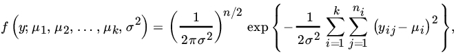
and, under H0,by

It is easy to check that the MLEs are


and

By Theorem 12.2.1, the likelihood ratio test is to reject H0 if

where F0 is the upper α percent point in the ![]() distribution. Since
distribution. Since

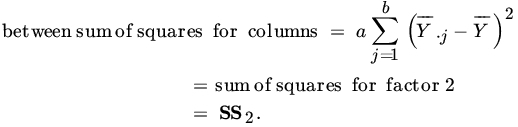
we may rewrite (9) as

It is usual to call the sum of squares in the numerator of (11) the between sum of squares (BSS) and the sum of squares in the denominator of (11) the within sum of squares (WSS). The results are conveniently displayed in a so-called analysis of variance table in the following form.
| One-Way Analysis of Variance | |||||
|
Source Variation |
Sum of Squares | Degrees of Freedom | Mean Sum of Squares | F-Ratio | |
| Between |  |
BSS/(k–1) | 
|
||
| Within |  |
||||
| Mean | 1 | ||||
| Total | 
|
n | |||
The third row, designated “Mean,” has been included to make the total of the second column add up to the total sum of squares (TSS), ![]()
From the data ![]() , and
, and

Also, the grand mean is
Thus

| Analysis of Variance | ||||
| Source | SS | d.f. | MSS | F-Ratio |
| Between | 1140 | 2 | 570 | |
| Within | 1600 | 12 | 133.33 | |
Choosing ![]() , we see that
, we see that ![]() . Thus we reject
. Thus we reject ![]() at level
at level ![]() .
.
From the data ![]() ,
, ![]() ,
, ![]() . Also, the grand mean is
. Also, the grand mean is
Thus

| Analysis of Variance | ||||
| Source | SS | d.f. | MSS | F-Ratio |
| Between | 303.41 | 2 | 151.70 | 151.70/489.67 |
| Within | 11,752.00 | 24 | 489.67 | |
We therefore cannot reject the null hypothesis that the average grades given by the three instructors are the same.
PROBLEMS 12.4
- Prove statements (5), (6), (7), and (8).
- The following are the coded values of the amounts of corn (in bushels per acre) obtained from four varieties, using unequal number of plots for the different varieties:

Test whether there is a significant difference between the yields of the varieties.
- A consumer interested in buying a new car has reduced his search to six different brands: D, F, G, P, V, T. He would like to buy the brand that gives the highest mileage per gallon of regular gasoline. One of his friends advises him that he should use some other method of selection, since the average mileages of the six brands are the same, and offers the following data in support of her assertion.
Distance Traveled (Miles) per Gallon of Gasoline Brand Car D F G P V T 1 42 38 28 32 30 25 2 35 33 32 36 35 32 3 37 28 35 27 25 24 4 37 37 26 30 5 28 30 6 19 Should the consumer accept his friend's advice?
- The following data give the ages of entering freshmen in independent random samples from three different universities.
University A B C 17 16 21 19 16 23 20 19 22 21 20 18 19 Test the hypothesis that the average ages of entering freshman at these universities are the same.
- Five cigarette manufacturers claim that their product has low tar content. Independent random samples of cigarettes are taken from each manufacturer and the following tar levels (in milligrams) are recorded.
Brand Tar Lavel (mg) A 4.2, 4.8, 4.6, 4.0, 4.4 B 4.9, 4.8, 4.7, 5.0, 4.9, 5.2 C 5.4, 5.3, 5.4, 5.2, 5.5 D 5.8, 5.6, 5.5, 5.4, 5.6, 5.8 E 5.9, 6.2, 6.2, 6.8, 6.4, 6.3 Can the differences among the sample means be attributed to chance?
- The quantity of oxygen dissolved in water is used as a measure of water pollution. Samples are taken at four locations in a lake and the quantity of dissolved oxygen is recorded as follows (lower reading corresponds to greater pollution):
Location Quantity of Dissolved Oxygen (%) A 7.8, 6.4, 8.2, 6.9 B 6.7, 6.8, 7.1, 6.9, 7.3 C 7.2, 7.4, 6.9, 6.4, 6.5 D 6.0, 7.4, 6.5, 6.9, 7.2, 6.8 Do the data indicate a significant difference in the average amount of dissolved oxygen for the four locations?
12.5 TWO-WAY ANALYSIS OF VARIANCE WITH ONE OBSERVATION PER CELL
In many practical problems one is interested in investigating the effects of two factors that influence an outcome. For example, the variety of grain and the type of fertilizer used both affect the yield of a plot or the score on a standard examination is influenced by the size of the class and the instructor.
Let us suppose that two factors affect the outcome of an experiment. Suppose also that one observation is available at each of a number of levels of these two factors. Let ![]() be the observation when the first factor is at the ith level, and the second factor at the jth level. Assume that
be the observation when the first factor is at the ith level, and the second factor at the jth level. Assume that
where αi is the effect of the ith level of the first factor, βj is the effect of the jth level of the second factor, and εij is the random error, which is assumed to be normally distributed with mean 0 and variance σ2. We will assume that the εij’s are independent. It follows that Yij are independent normal RVs with means ![]() and variance σ2. There is no loss of generality in assuming that
and variance σ2. There is no loss of generality in assuming that ![]() for, if
for, if ![]() , we can write
, we can write

and ![]() Here we have written
Here we have written ![]() and
and ![]() for the means of
for the means of ![]() ’s and
’s and ![]() ’s, respectively. Thus Yij may denote the yield from the use of the ith variety of some grain and the jth type of some fertilizer. The two hypotheses of interest are
’s, respectively. Thus Yij may denote the yield from the use of the ith variety of some grain and the jth type of some fertilizer. The two hypotheses of interest are
The first of these, for example, says that the first factor has no effect on the outcome of the experiment.
In view of the fact that ![]() and
and ![]() and we can write our model in matrix notation as
and we can write our model in matrix notation as
where

and

The vector of unknown parameters β is ![]() and the matrix X is
and the matrix X is ![]() (b blocks of a rows each). We leave the reader to check that X is of full rank,
(b blocks of a rows each). We leave the reader to check that X is of full rank, ![]() . The hypothesis
. The hypothesis ![]() or
or ![]() can easily be put into the form
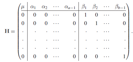
can easily be put into the form ![]() . For example, for Hβ we can choose H to be the
. For example, for Hβ we can choose H to be the ![]() matrix of full rank
matrix of full rank ![]() , given by
, given by
Clearly, the model described above is a special case of the general linear hypothesis, and we can use Theorem 12.2.1 to test Hβ.
To apply Theorem 12.2.1 we need the estimators ![]() and
and ![]() . It is easily checked that
. It is easily checked that

and
where ![]() Also, under Hβ, for example,
Also, under Hβ, for example,
In the notation of Theorem 12.2.1, ![]() , so that
, so that ![]() , and
, and

Since

we may write

It follows that, under ![]() has a central
has a central ![]() distribution.
distribution.
The numerator of F in (8) measures the variability between the means ![]() and the denominator measures the variability that exists once the effects due to the two factors have been subtracted.
and the denominator measures the variability that exists once the effects due to the two factors have been subtracted.
If Hα is the null hypothesis to be tested, one can show that under Hα the MLEs are
As before, ![]() , but
, but ![]() . Also,
. Also,
which may be rewritten as

It follows that, under ![]() F has a central
F has a central ![]() distribution. The numerator of F in (11) measures the variability between the means
distribution. The numerator of F in (11) measures the variability between the means ![]() .
.
If the data are put into the following form:

so that the rows represent various levels of factor 1, and the columns, the levels of factor 2, one can write

Similarly,
It is usual to write error or residual sum of squares (SSE) for the denominator of (8) or (11). These results are conveniently presented in an analysis of variance table as follows.
| Two-Way Analysis of Variance Table with One Observation per Cell | ||||
| Source of Variation | Sum of Squares | Degrees of Freedom | Mean Square | F-Ratio |
| Rows | SS1 | MS1/MSE | ||
| Columns | SS2 | MS2/MSE | ||
| Error | SSE | |||
| Mean | 1 | |||
| Total | 
|
ab | 
|
|
In our notation, ![]() ,
, ![]() ,
, ![]() ,
, ![]() ,
, ![]() ,
, ![]() ,
, ![]() ,
, ![]() ,
, ![]() ,
, ![]() .
.
Also,


The results are shown in the following table:
| Analysis of Variance | ||||
| Source | SS | d.f. | MS | F-Ratio |
| Variety of wheat | 34.67 | 2 | 17.33 | 14.2 |
| Fertilizer | 4.67 | 3 | 1.56 | 1.28 |
| Error | 7.33 | 6 | 1.22 | |
| Mean | 481.33 | 1 | 481.33 | |
| Total | 528.00 | 12 | 44.00 | |
Now ![]() and
and ![]() . Since
. Since ![]() , we reject Hβ, that there is equality in the average yield of the three varieties; but, since
, we reject Hβ, that there is equality in the average yield of the three varieties; but, since ![]() , we accept Hα, that the four fertilizers are equally effective.
, we accept Hα, that the four fertilizers are equally effective.
PROBLEMS 12.5
- Show that the matrix X for the model defined in (2) is of full rank,
 .
. - Prove statements (3), (4), (5), and (9).
- The following data represent the units of production per day turned out by four different brands of machines used by four machinists:
Machinist Machine A1 A2 A3 A4 B1 15 14 19 18 B2 17 12 20 16 B3 16 18 16 17 B4 16 16 15 15 Test whether the differences in the performances of the machinists are significant and also whether the differences in the performances of the four brands of machines are significant. Use
 .
. - Students were classified into four ability groups, and three different teaching methods were employed. The following table gives the mean for four groups:
Teaching Method Ability Group A B C 1 15 19 14 2 18 17 12 3 22 25 17 4 17 21 19 Test the hypothesis that the teaching methods yield the same results. That is, that the teaching methods are equally effective.
- The following table shows the yield (pounds per plot) of four varieties of wheat, obtained with three different kinds of fertilizers.
Variety of Wheat Fertilizer A B C D α 8 3 6 7 β 10 4 5 8 γ 8 4 6 7 Test the hypotheses that the four varieties of wheat yield the same average yield and that the three fertilizers are equally effective.
12.6 TWO-WAY ANALYSIS OF VARIANCE WITH INTERACTION
The model described in Section 12.5 assumes that the two factors act independently, that is, are additive. In practice this is an assumption that needs testing. In this section we allow for the possibility that the two factors might jointly affect the outcome, that is, there might be so-called interactions. More precisely, if Yij is the observation in the (i,j)th cell, we will consider the model
where ![]() represent row effects (or effects due to factor 1),
represent row effects (or effects due to factor 1), ![]() represent column effects (or effects due to factor 2), and γij represent interactions or joint effects. We will assume that εij are independently
represent column effects (or effects due to factor 2), and γij represent interactions or joint effects. We will assume that εij are independently ![]() (0,σ2). We will further assume that
(0,σ2). We will further assume that
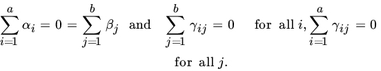
The hypothesis of interest is
One may also be interested in testing that all α’s are 0 or that all β’s are 0 in the presence of interactions γij.
We first note that (2) is not restrictive since we can write
where ![]() , and
, and ![]() do not satisfy (2), as
do not satisfy (2), as

and then (2) is satisfied by choosing

Here

Next note that, unless we replicate, that is, take more than one observation per cell, there are no degrees of freedom left to estimate the error SS (see Remark 1).
Let Yijs be the sth observation when the first factor is at the ith level, and the second factor at the jth level, ![]() . Then the model becomes as follows:
. Then the model becomes as follows:
| Levels of Factor 1 | ||||
| Levels of Factor 2 | 1 | 2 | … | b |
| 1 | y111 | y121 | … | y1b1 |
| ∙ | ∙ | … | ∙ | |
| ∙ | ∙ | … | ∙ | |
| ∙ | ∙ | … | ∙ | |
| y11m | y12m | … | y1bm | |
| 2 | y211 | y221 | … | y2b1 |
| ∙ | ∙ | … | ∙ | |
| ∙ | ∙ | … | ∙ | |
| ∙ | ∙ | … | ∙ | |
| y21m | y22m | … | y2bm | |
| ∙ | ∙ | … | ∙ | |
| ∙ | ∙ | … | ∙ | |
| ∙ | ∙ | … | ∙ | |
| a | ya11 | ya21 | … | yab1 |
| ∙ | ∙ | … | ∙ | |
| ∙ | ∙ | … | ∙ | |
| ∙ | ∙ | … | ∙ | |
| ya1m | ya2m | … | yabm | |
![]() , and
, and ![]() , where εijs’s are independent
, where εijs’s are independent ![]() (0,σ2). We assume that
(0,σ2). We assume that ![]() . Suppose that we wish to test
. Suppose that we wish to test ![]() . We leave the reader to check that model (4) is then a special case of the general linear hypothesis with
. We leave the reader to check that model (4) is then a special case of the general linear hypothesis with ![]() , and
, and ![]() .
.
Let us write

Then it can be easily checked that

It follows from Theorem 12.2.1 that

Since

we can write (7) as

Under Hα the statistic ![]() has the central
has the central ![]() distribution, so that the likelihood ratio test rejects Hα if
distribution, so that the likelihood ratio test rejects Hα if

A similar analysis holds for testing ![]() .
.
Next consider the test of hypothesis ![]() for all i, j, that is, that the two factors are independent and the effects are additive. In this case
for all i, j, that is, that the two factors are independent and the effects are additive. In this case ![]() , and
, and ![]() . It can be shown that
. It can be shown that
Thus
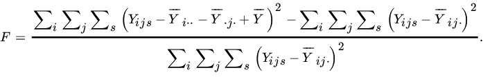
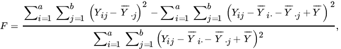
Now

so that we may write

Under Hγ, the statistic ![]() has the
has the ![]() distribution. The likelihood ratio test rejects Hγ if
distribution. The likelihood ratio test rejects Hγ if

Let us write
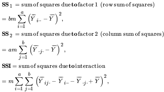
and

Then we may summarize the above results in the following table.
| Two-Way Analysis of Variance Table with Interaction | ||||
| Source of Variation | Sum of Squares | Degrees of Freedom | Mean Square | F-Ratio |
| Rows | SS1 | MS1/MSE | ||
| Columns | SS2 | MS2/MSE | ||
| Interaction | SSI | MSI/MSE | ||
| Error | SSE | |||
| Mean | 1 | |||
| Total | 
|
abm | 
|
|
Remark 1. Note that, if ![]() , there are no d.f. associated with the SSE. Indeed, SSE
, there are no d.f. associated with the SSE. Indeed, SSE ![]() if
if ![]() Hence, we cannot make tests of hypotheses when
Hence, we cannot make tests of hypotheses when ![]() , and for this reason we assume
, and for this reason we assume ![]() .
.
| Instructor | |||
| Teaching Method | I | II | III |
| 1 | 95 | 60 | 86 |
| 85 | 90 | 77 | |
| 74 | 80 | 75 | |
| 74 | 70 | 70 | |
| 2 | 90 | 89 | 83 |
| 80 | 90 | 70 | |
| 92 | 91 | 75 | |
| 82 | 86 | 72 | |
| 3 | 70 | 68 | 74 |
| 80 | 73 | 86 | |
| 85 | 78 | 91 | |
| 85 | 93 | 89 | |
From the data the table of means is as follows:
| 82 | 75 | 77 | 78.0 | |
| 86 | 89 | 75 | 83.3 | |
| 80 | 78 | 85 | 81.0 | |
| 82.7 | 80.7 | 79.0 | ||
Then

| Analysis of Variance | ||||
| Source | SS | d.f. | MSS | F-Ratio |
| Methods | 169.56 | 2 | 84.78 | 1.25 |
| Instructors | 82.32 | 2 | 41.16 | 0.61 |
| Interactions | 561.80 | 4 | 140.45 | 2.07 |
| Error | 1830.00 | 27 | 67.78 | |
With ![]() , we see from the tables that
, we see from the tables that ![]() and
and ![]() , so that we cannot reject any of the three hypotheses that the three methods are equally effective, that the three instructors are equally effective, and that the interactions are all 0.
, so that we cannot reject any of the three hypotheses that the three methods are equally effective, that the three instructors are equally effective, and that the interactions are all 0.
PROBLEMS 12.6
- Prove statement (6).
- Obtain the likelihood ratio test of the null hypothesis
 .
.
- Prove statement (10).
- Suppose that the following data represent the units of production turned out each day by three different machinists, each working on the same machine for three different days:
Machinist Machine A B C B1 15, 15, 17 19, 19, 16 16, 18, 21 B2 17, 17, 17 15, 15, 15 19, 22, 22 B3 15, 17, 16 18, 17, 16 18, 18, 18 B4 18, 20, 22 15, 16, 17 17, 17, 17 Using a 0.05 level of significance, test whether (a) the differences among the machinists are significant, (b) the differences among the machines are significant, and (c) the interactions are significant.
- In an experiment to determine whether four different makes of automobiles average the same gasoline mileage, a random sample of two cars of each make was taken from each of four cities. Each car was then test run on 5 gallons of gasoline of the same brand. The following table gives the number of miles traveled.
Automobile Make Cities A B C D Cleveland 92.3, 104.1 90.4, 103.8 110.2, 115.0 120.0, 125.4 Detroit 96.2, 98.6 91.8, 100.4 112.3, 111.7 124.1, 121.1 San Francisco 90.8, 96.2 90.3, 89.1 107.2, 103.8 118.4, 115.6 Denver 98.5, 97.3 96.8, 98.8 115.2, 110.2 126.2, 120.4 Construct the analysis of variance table. Test the hypothesis of no automobile effect, no city effect, and no interactions. Use
 .
.