
8
Fractional Differentiation
8.1. Introduction
Fractional calculus is generally referred to the fractional derivatives of Riemann–Liouville and Caputo [DIE 10]. Paradoxically, from the beginning of this book, we have addressed fractional calculus only with the definition of the Riemann–Liouville integral and the fractional integrator ![]() Fractional differentiation is mentioned only through its Laplace transform sn and with the Grünwald–Letnikov derivative. This surprising approach is motivated by the definition of fractional differentiation which requires the integer order differentiation and the fractional order integration [TRI 13d]. Moreover, the use of Riemann–Liouville or Caputo derivatives requires us to specify their initial conditions [POD 99]. However, as we will demonstrate it, these initial conditions require us to introduce the initial state of the associated Riemann–Liouville integral. Consequently, usual initial conditions of these derivatives have to be revisited [HAR 09a, LOR 11], as highlighted by many research works [SAB 10a, TRI 10b, TRI 13a, TRI 15].
Fractional differentiation is mentioned only through its Laplace transform sn and with the Grünwald–Letnikov derivative. This surprising approach is motivated by the definition of fractional differentiation which requires the integer order differentiation and the fractional order integration [TRI 13d]. Moreover, the use of Riemann–Liouville or Caputo derivatives requires us to specify their initial conditions [POD 99]. However, as we will demonstrate it, these initial conditions require us to introduce the initial state of the associated Riemann–Liouville integral. Consequently, usual initial conditions of these derivatives have to be revisited [HAR 09a, LOR 11], as highlighted by many research works [SAB 10a, TRI 10b, TRI 13a, TRI 15].
Let us finally recall that the usual approach to the analysis of fractional systems dynamics is based on the properties of these derivatives, particularly on their initial conditions [MAT 96, BET 06, MON 10]. As demonstrated in Chapter 7, FDS transients can be expressed with the initial conditions of internal integrators. Therefore, we intend to demonstrate that FDS transients are independent of the type of fractional differentiation used to analyze them. Finally, numerical simulations will illustrate the transients of Riemann–Liouville and Caputo derivatives.
8.2. Implicit fractional differentiation
Let us consider Figure 8.1: as x(t) is the output of the operator ![]() its input v(t) is equal to the implicit fractional derivative
its input v(t) is equal to the implicit fractional derivative ![]() (I for implicit).
(I for implicit).
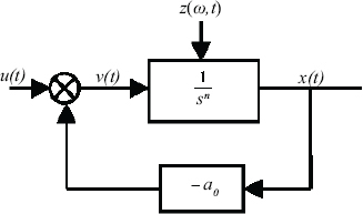
Figure 8.1. Analog simulation of the one-derivative FDS
Of course, for initial conditions equal to 0 at t = 0 , we can write:
which can also be interpreted as:
or using the Laplace transform:
i.e.
Let us define:
where:
Then, equation [8.1] can be interpreted as:
where h−n(t) is called the convolution inverse of hn(t) [MAT 94].
It is important to note that the fractional integration process of Figure 8.1 is not a reversible operation: we obtain ![]() only inside the closed loop of Figure 8.1, used for the simulation of:
only inside the closed loop of Figure 8.1, used for the simulation of:
We can conclude that the implicit fractional derivative:
- – corresponds to the input of the fractional integrator;
- – can be interpreted as the convolution of x(t) with the impulse response h−n(t).
As demonstrated in the previous chapters, implicit derivative plays a fundamental role in the analysis of FDS dynamics.
8.3. Explicit Riemann–Liouville and Caputo fractional derivatives
8.3.1. Definitions
The modeling of FDSs was presented in Chapter 7, with fractional orders ni verifying 0 < ni ≤ 1.
Therefore, we are interested principally in the properties of Riemann–Liouville and Caputo derivatives for 0 < n < 1.
The fractional derivative of a function f(t) was defined as Dn(f(t)) in Chapter 1, using the Laplace transform and for initial conditions equal to 0:
Equation [8.4] can be written as:
or
Equation [8.10] corresponds to:
where ![]() is the Caputo derivative, whereas equation [8.11] corresponds to:
is the Caputo derivative, whereas equation [8.11] corresponds to:
where ![]() is the Riemann–Liouville derivative.
is the Riemann–Liouville derivative.
For each derivative, ![]() is the Riemann–Liouville integral of the order 1 − n associated with integer order differentiation.
is the Riemann–Liouville integral of the order 1 − n associated with integer order differentiation.
REMARK 1.– These definitions are easily generalized to any value n:
N − 1 < n < N, where N is an integer.
As we can write:
therefore
and
We can note that these two derivatives are based on the fractional integration of the order ![]() where
where ![]()
Thus, as noted previously, the fractional integration is of the order ![]() whereas associated integer order differentiation is of the order N.
whereas associated integer order differentiation is of the order N.
8.3.2. Theoretical prerequisites
The thereafter analysis of the different fractional derivatives relies on a fundamental assumption: we assume the existence of ![]() which is the exact fractional derivative of f(t).
which is the exact fractional derivative of f(t).
We define three derivatives, ![]() in order to compute or calculate
in order to compute or calculate ![]()
Due to initial conditions at t = 0 which will be specified afterwards, implicit and explicit fractional derivatives provide different values of ![]() which is one of the major problems of fractional calculus [ORT 08, ORT 11].
which is one of the major problems of fractional calculus [ORT 08, ORT 11].
In order to get rid of these initial conditions at t = 0 (or at t = t0), we define these derivatives since t = −∞, i.e. the associated integrals are defined since t = −∞.
Let us recall that ![]()
Therefore, for the implicit derivative:
note that ![]() is the input of the fractional integrator
is the input of the fractional integrator ![]() delivering
delivering ![]() since t = −∞ with:
since t = −∞ with:
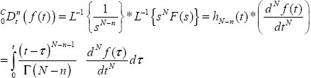
For the Caputo derivative:
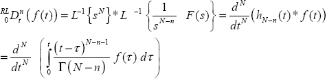
and for the Riemann–Liouville derivative:

Because these three expressions of Dn(f) are calculated since t = −∞, the possible transients caused by initial conditions at t = −∞ have completely vanished at instant t. Therefore, these derivatives are equal at instant t to the fractional derivative Dn(f):
Of course, this equality is not verified for ![]()
8.3.3. Comments
Fractional differentiation obeys different definitions, unlike the integer order case, where the definition is unique. Moreover, it is important to note that each of these definitions is related to fractional integration, of the order n for the implicit derivative and of the order 1 − n for the Caputo and Riemann–Liouville derivatives.
The role of this fractional integration in the usual approach to fractional differentiation is untold. On the contrary, this fractional integration plays an essential role in the analysis of transients. It is one of the paradoxes of fractional calculus where focus is put on fractional differentiation, whereas it will be necessary to concentrate on fractional integration. Moreover, it is the cause of wrong formulations of fractional derivative initial conditions, as we will prove it in the next section.
8.4. Initial conditions of fractional derivatives
8.4.1. Introduction
It has been demonstrated that ![]() provide the same value
provide the same value ![]() at any instant t.
at any instant t.
Practically, these derivatives are calculated since an instant t0 (t0 = 0 afterwards), so we will consider ![]() Because these derivatives depend on a specific Riemann–Liouville integral, this integration process introduces distributed states zI(ω,t0), zC(ω,t0) or zRL(ω,t0). Equality of the three derivatives at any instant t is necessarily related to these distributed states.
Because these derivatives depend on a specific Riemann–Liouville integral, this integration process introduces distributed states zI(ω,t0), zC(ω,t0) or zRL(ω,t0). Equality of the three derivatives at any instant t is necessarily related to these distributed states.
Practically, because the Laplace transform is defined for t ≥ 0, the equality of the derivative Laplace transforms will be expressed at initial instant t0 = 0.
Moreover, because the initial conditions of the derivatives are formulated in the framework of FDS, we first consider the one-derivative case, which we will generalize to N -derivative FDSs in the next section.
Let
be the one-derivative FDS (or FDE).
We assume that u(t) is applied to the elementary system since t = −∞
8.4.2. Implicit derivative
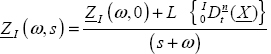
Let x(t) be the output of the fractional integrator ![]() (see Figure 8.1). The input of the integrator provides the implicit derivative and its internal state z(ω,0) = zI(ω,0) at instant t0 = 0 . zI(ω,0) summarizes the past of the system, i.e. the influence at t = 0 of u(t) since t = −∞.
(see Figure 8.1). The input of the integrator provides the implicit derivative and its internal state z(ω,0) = zI(ω,0) at instant t0 = 0 . zI(ω,0) summarizes the past of the system, i.e. the influence at t = 0 of u(t) since t = −∞.
Now, if we start the integration process at t0 = 0, we obtain ![]() The dynamics of the fractional integrator verify the distributed differential system:
The dynamics of the fractional integrator verify the distributed differential system:

where zI(ω,0) is the distributed initial state.
If the fractional integrator is initialized with zI(ω,0), we obtain the initialized implicit derivative ![]()
Using the Laplace transform, we can write:
Therefore
Thus, we finally obtain:
8.4.3. Caputo derivative
The Caputo derivative, calculated since t = −∞, i.e. ![]() is provided by a fractional integrator of the order (1 − n) excited by the integer order derivative
is provided by a fractional integrator of the order (1 − n) excited by the integer order derivative ![]() according to Figure 8.2.
according to Figure 8.2.
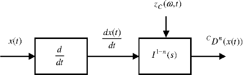
Figure 8.2. Caputo derivative principle
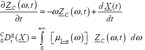
zc(ω,t) is the distributed state associated with ![]() note that it is different from zI(ω,t) (or zRL(ω,t)).
note that it is different from zI(ω,t) (or zRL(ω,t)).
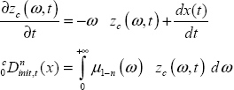
Let zc(ω,0) be the value at t = 0, summarizing the past behavior of the integrator (t < 0). The dynamics of ![]() verify the distributed differential system:
verify the distributed differential system:
Let ![]() be the initialized Caputo derivative calculated since t = 0, where the integrator
be the initialized Caputo derivative calculated since t = 0, where the integrator ![]() has been initialized by zc(ω,0).
has been initialized by zc(ω,0).
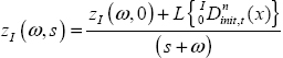
The Laplace transform provides:
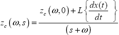
we obtain:
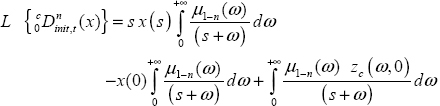
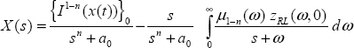
As ![]() we finally obtain:
we finally obtain:
REMARK 2.– The commonly accepted definition of Caputo’s initial conditions [POD 99] is expressed as:
There is a serious problem with this definition because it does not take into account the distributed state of the fractional integrator ![]() at t = 0.
at t = 0.
x(0) cannot be interpreted as the initial condition of the Caputo derivative: equation [8.31] clearly exhibits that these initial conditions are x(0) and zc(ω,0). The same problem exists with the Riemann–Liouville derivative.
8.4.4. Riemann–Liouville derivative
The Riemann–Liouville derivative, calculated since t = −∞, i.e. ![]() is provided by the integer order derivative of the output of the fractional integrator
is provided by the integer order derivative of the output of the fractional integrator ![]() according to Figure 8.3.
according to Figure 8.3.
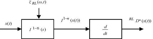
Figure 8.3. Riemann–Liouville derivative principle
zRL(ω,t) is the distributed state associated with ![]() and zRL(ω,0) summarizes the past behavior of the integrator (for t < 0).
and zRL(ω,0) summarizes the past behavior of the integrator (for t < 0).
The dynamics of ![]() verify the distributed differential system:
verify the distributed differential system:

Let ![]() be the initialized Riemann–Liouville derivative calculated since t = 0, where the integrator
be the initialized Riemann–Liouville derivative calculated since t = 0, where the integrator ![]() is initialized by zRL(ω,0).
is initialized by zRL(ω,0).
The Laplace transform provides:
where ![]()
Therefore, we finally obtain:
REMARK 3.– The initial conditions of Riemann–Liouville and Caputo derivatives have motivated several interpretations (see, for example, [POD 02a, TRI 10b]).
8.4.5. Relations between initial conditions
The previous three equations correspond to the initialized fractional derivatives. These initialized derivatives provide the exact value of ![]() since the influence of the past (t < 0) is summarized by the initial conditions.
since the influence of the past (t < 0) is summarized by the initial conditions.
Therefore, by equality of the Laplace transforms of the three derivatives, we can formulate the relations between the different initial conditions.
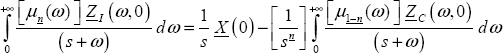
8.4.5.1. Relation between the implicit and Caputo initial conditions
Therefore, we obtain
8.4.5.2. Relation between the implicit and Riemann–Liouville initial conditions
Equality of Laplace transforms provides:
8.5. Initial conditions in the general case
8.5.1. Introduction
Let us consider the N -derivative FDS:
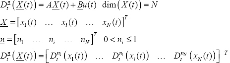
We use the same procedure as with N = 1. The three derivatives are calculated since t = −∞, and we use the Laplace transform to infer relations between the initial conditions at t = 0.
8.5.2. Implicit derivatives
The implicit derivative ![]() corresponds to the input of the fractional integrator
corresponds to the input of the fractional integrator ![]() operating since t = 0.
operating since t = 0.
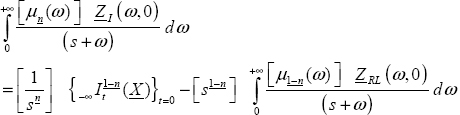
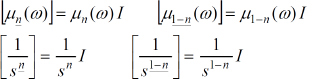
Let ZI(ω,t) be the distributed state variables of the integrators and ZI(ω,0) their initial conditions at t0 = 0 .
Then:

Therefore
Thus, we obtain:
![]() were defined in Chapter 7.
were defined in Chapter 7.
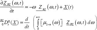
8.5.3. Caputo derivatives
![]() is defined as:
is defined as:
Let ZC(ω,t) be the distributed state variable of the integrators ![]() (i = 1 to N) and ZC(ω,0) be their initial conditions at t0 = 0 .
(i = 1 to N) and ZC(ω,0) be their initial conditions at t0 = 0 .
Then:
Therefore:
Thus:
8.5.4. Riemann–Liouville derivatives
![]() is defined as:
is defined as:

Let ZRL(ω,t) be the distributed state variable of the integrators ![]() (i = 1 to N) and ZRL(ω,0) be their initial conditions at t0 = 0 .
(i = 1 to N) and ZRL(ω,0) be their initial conditions at t0 = 0 .
Then:
Therefore:
Thus:

8.5.5. Relations between initial conditions
As in the one-derivative case, we obtain the following.
8.5.5.1. Relation between the implicit and Caputo initial conditions
8.5.5.2. Relation between the implicit and Riemann–Liouville initial conditions
In the commensurate order case (i.e. n1 = ... = ni = ... = nN), these relations are simplified since:
8.6. Unicity of FDS transients
8.6.1. Transients of the elementary FDE
Consider the elementary FDE:
We can express the free response using each of the fractional derivatives and their respective initial conditions. Therefore, we obtain three expressions of x(t): xI(t), xC(t), xRL(t):
l) For the implicit derivative: ![]() the initial condition is zI(ω,0).
the initial condition is zI(ω,0).
Then, we obtain for the free response (u(t) = 0):
Using equation [8.26], we finally obtain:
Note that this result corresponds to equation [7.8] because zI(ω,0) = z(ω,0).
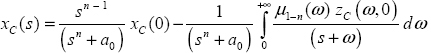
2) For the Caputo derivative: ![]() the initial conditions are xC(0) and zC(ω,0). Then, we obtain for the free response:
the initial conditions are xC(0) and zC(ω,0). Then, we obtain for the free response:
Using [8.31], we finally obtain:
3) For the Riemann–Liouville derivative: ![]() and the initial conditions are
and the initial conditions are ![]() Then, we obtain for the free response:
Then, we obtain for the free response:
Using [8.36], we finally obtain:
8.6.2. Unicity of transients
The true “physical” free response of the FDE depends only on its initial condition and obviously cannot depend on the choice of the fractional derivative used to analyze the FDE.
However, the three responses xI(t), xC(t) and xRL(t) seem to be different because of specific initial conditions.
In fact, we have determined relations between these initial conditions.
Consider, for example, xI(t) and xC(t):
Using relation [8.38] between the implicit and Caputo initial conditions, we obtain:

This means that
where x(t) is the free response expressed in Chapter 7.
Applying the same approach to xRL(t), it is straightforward to obtain
- xI(t) = xRL(t) = x(t)
Therefore, we can conclude that: xI(t) = xC(t) = xRL(t) = x(t). i.e. there is unicity of the free responses calculated with the different fractional derivatives.
Obviously, this result applies directly to an N -derivative FDS, using relations [8.52] and [8.53].
8.6.3. Conclusion
We can use either ![]() to express the free response of:
to express the free response of:
since we have proved the equivalence of XI(t), XC(t) or XRL(t).
Nevertheless, there is a fundamental difficulty to express XC(t) or XRL(t).
Note that ZI(ω,0) = Z(ω,0) is a “natural” initial condition because it is intrinsically linked to fractional integrators ![]() i.e. ZI(ω,0) is directly available and its interpretation is straightforward.
i.e. ZI(ω,0) is directly available and its interpretation is straightforward.
On the contrary, ZC(ω,0) and ZRL(ω,0) are not directly available because they require the calculation of the corresponding fractional derivatives with integrators ![]() Moreover, their interpretation in terms of
Moreover, their interpretation in terms of ![]() dynamics, i.e. of system dynamics, is not straightforward (see section 8.7).
dynamics, i.e. of system dynamics, is not straightforward (see section 8.7).
It is necessary to remember that the Caputo derivative has motivated an unjustified interest due to the apparent simplicity of equation [8.32]. It has been interpreted as a strong similitude between the integer order derivative and the Caputo derivative, where x(0) has been interpreted as a physical initial condition of this derivative.
Consequently, the free response of ![]() is expressed as:
is expressed as:
This expression is obviously wrong, as it is illustrated by the numerical simulation of section 8.7.
Expression [8.26] using ZI(ω,0) = Z(ω,0) is not as simple as its erroneous homolog [8.32], but it is the price to pay in fractional calculus, where dynamical transients are more complex than in the integer order case.
Finally, let us highlight that ZI(ω,t) = Z(ω,t) generalizes the concept of the integer order state variable to the fractional order case:
– X(t) is the state vector for integer order systems;
– X(t) is the pseudo-state vector, whereas Z(ω,t) is the distributed state vector for fractional order systems.
8.7. Numerical simulation of Caputo and Riemann–Liouville transients
8.7.1. Introduction
Unicity of FDS transients was proved in the previous section. Nevertheless, it is interesting to verify this fundamental result by numerical simulations.
Therefore, the purpose is to illustrate that the transients of an elementary one-derivative FDE, expressed either with the Caputo derivative or the Riemann–Liouville derivative, are identical to the transients expressed with the implicit derivative, i.e. with the distributed variable z(ω,t).
8.7.2. Simulation of Caputo derivative initialization
Consider the elementary system [8.22]:
The input of the system is:
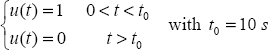
The system internal state zI(ω,t) is equal to 0 at t = 0 .
Then, at t = t0, this internal state is zI (ω,t0).
As u(t) = 0 for t > t0, we observe the free response of the system, initialized by zI(ω,t0): the response x(t) is presented in Figure 8.5.
In order to initialize this system with the Caputo derivative, we must compute
At t = t0, we obtain x(t0) and zC(ω,t0) (internal state of I1−n(s)).
Let us recall equation [8.59] with t0 = 0 :
Let us define:
and
- Then, for t ≥ t0:
This term is usually considered as the free response of the system, initialized by x(t0) [LES 11].
Of course, this solution does not work because there is a transient, even though x(t0) = 0!
Therefore, it is necessary to use the supplementary term:
![]() is the free response of the I1−n(s) integrator, with the initial condition zC(ω,0), and xz,Cap(t) is the response of
is the free response of the I1−n(s) integrator, with the initial condition zC(ω,0), and xz,Cap(t) is the response of ![]() to this free response, according to Figure 8.4.
to this free response, according to Figure 8.4.
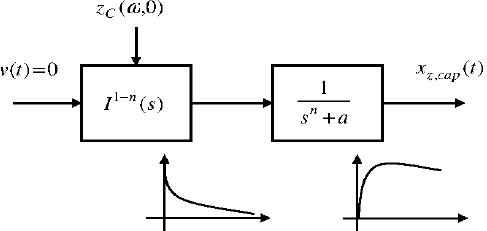
Figure 8.4. Analysis of the Caputo supplementary term
Finally
These two signals are plotted in Figure 8.5.
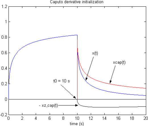
Figure 8.5. Simulation of Caputo derivative initialization. For a color version of this figure, see www.iste.co.uk/trigeassou/analysis1.zip
Obviously, xCap(t) is different from x(t), although they share the same starting point x(t0).
Finally, if we add −xz, Cap(t) to xCap(t), we exactly obtain x(t).
Therefore, it is possible to correctly initialize the FDS with the Caputo derivative, but the procedure is more complex than the direct one, based only on zI(ω,t0) = z(ω,t0).
8.7.3. Simulation of Riemann–Liouville initialization
We consider the same system [8.22] and use the same procedure as described previously.
First, we must compute I1−n(x(t)) and differentiate this integral to obtain
At t = t0, we obtain ![]() and zRL(ω,t0) (state of I1−n(s)).
and zRL(ω,t0) (state of I1−n(s)).
Let us recall equation [8.61] with t0 = 0 :
Let us define:

and
Then
This term is called the Riemann–Liouville free response [LES 11].
Of course, it cannot fit the true free response because xRL(t) → ∞ when t → t0.
Therefore, it is necessary to use the supplementary term:
![]() is the free response of the I1−n(s) integrator, with the initial condition zRL(ω,0), and xz, RL(t) is the integer derivative of the response of
is the free response of the I1−n(s) integrator, with the initial condition zRL(ω,0), and xz, RL(t) is the integer derivative of the response of ![]() to this free response, according to Figure 8.6.
to this free response, according to Figure 8.6.
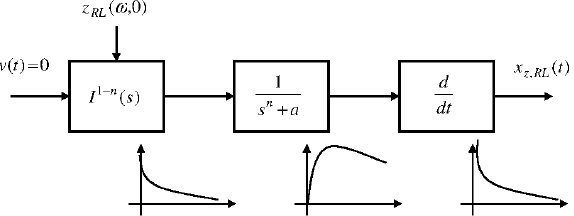
Figure 8.6. Analysis of the Riemann–Liouville supplementary term
Note that xz, RL(t) → ∞ when t → t0 because of the integer derivative action.
These two signals are plotted in Figure 8.7 with x(t).
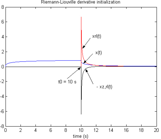
Figure 8.7. Simulation of Riemann–Liouville derivative initialization
First, we note an important change in the amplitude scale in comparison with Figure 8.5: because of the integer derivative action, the signals xRL(t) and xz, RL(t) are larger than x(t), particularly for ![]() Nevertheless, when we add −xz, RL(t) to xRL(t), we exactly obtain x(t).
Nevertheless, when we add −xz, RL(t) to xRL(t), we exactly obtain x(t).
Therefore, it is possible to initialize the FDS with the Riemann–Liouville derivative, with a similar procedure to the Caputo derivative and the conclusion is the same as summarized previously. We can use either the Caputo derivative or the Riemann–Liouville derivative to initialize the FDS, but the two procedures are obviously more complex than the direct one, based only on zI(ω,t0) = z(ω,t0)!