
4
Fractional Modeling of the Diffusive Interface
4.1. Introduction
Many physical and chemical processes, such as heat transfer in materials [BAT 01], eddy currents in electrical machines [RET 99], electrochemistry in batteries [SAB 06] and so on, are governed by diffusive partial derivative equations.
Practically, we are mainly concerned by the modeling of the diffusive interface at the boundary of the considered process, such as the voltage/current relationship in an accumulator [LIN 00] or the temperature/heat flux for heat transfer [BEN 06].
It has been demonstrated long ago [OLD 74] that the diffusive interface is characterized by a fractional order behavior in the frequency domain with n = 0.5. It is for this reason that a great number of research works have been devoted to the fractional modeling of diffusive interfaces, using various fractional order models [COI 01, LIN 01a]. Some of these models are motivated by physical properties [BAT 02], but many others are only identification (or black box) models motivated by the efficiency of the approximation.
Therefore, in this chapter, our purpose is to investigate why fractional models are adapted to the modeling of diffusive interfaces, and whether any fractional model can provide a correct physical response to this problem [MAA 15].
In order to formulate an objective response, we use a prototype interface, i.e. heat transfer in a plane wall.
Two families of fractional models are investigated: commensurate order models, which are derived from the truncation of the true transfer function, and non-commensurate order models, which are motivated by parsimony and physical reasons.
The commensurate order models are a direct and natural consequence of the truncation of the interface transfer function [BAT 02].
However, a good approximation of the diffusive interface requires a large truncation order. It is possible to improve this approximation with reduced model complexity based on parameter optimization, i.e. performing a frequency identification of the diffusive model.
An alternative to the truncation approach, in order to improve the parsimony objective, is to use a non-commensurate order model with a physical constraint. However, because this model is nonlinear in its parameters, a special optimization procedure is necessary to obtain its parameters by frequency identification.
Another objective is to highlight the “long memory” characteristic of the diffusive phenomenon, in connection with the thickness of the plane wall. Consequently, the fractional models have to reproduce this “long memory” behavior without introducing undesirable artifacts.
4.2. Heat transfer and diffusive model of the plane wall
4.2.1. Heat transfer
The evolution of the temperature in a heat conductive medium is governed by a partial derivative equation (PDE), called heat transfer [JOO 86, HOL 89].
Let us consider the case of conventional heat transfer [BEN 08a] through a uniform, homogeneous plane wall, with surface S and thickness L, heated on the face A by a heat flow ϕ(0,t) , while the face B is maintained at a constant temperature T(L,t) (see Figure 4.1).
Let ϕ(x,t) be the heat flow which crosses any plane parallel to the faces A and B located at the abscissa x of the wall (0 ≤ x ≤ L) , and T(x,t) be the temperature assumed to be uniform at each point of the plane.
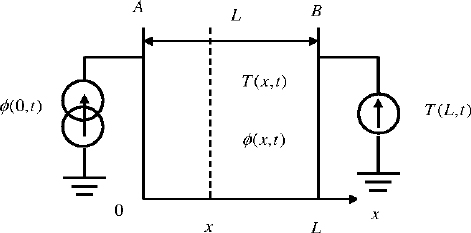
Figure 4.1. Diffusive interface: the plane wall case
Heat diffusion is expressed by the heat equation [4.1] which is a generalization of Fick’s law [OLD 70, FAR 82]:
where λ is the thermal conductivity, c is the specific heat, ρ is the mass density, ![]() is the thermal diffusivity and S is the surface area of the faces A and B.
is the thermal diffusivity and S is the surface area of the faces A and B.
Equation [4.2] expresses that the heat transfer corresponds to a flow ϕ which is proportional to the gradient of the temperature.
In the rest of this chapter, we will use the following numerical values [BEN 08a]: λ = 111 Wm−1K−1, ρ = 8.522 103 Kgm−1, c = 0.385 103 JKg−1K−1 and S = 10−2 m2.
4.2.2. Physical model of the diffusive interface
Let us consider the following boundary conditions.
Face A is subjected to an imposed and uniform heat flow ϕ(0,t) (power supply) over the entire surface S. It represents the system input u(t). The output is y(t) = T(0,t). On face B, a constant temperature is imposed (voltage source).
The initial condition (initial temperature profile) is:
As the model is developed around an operating point, the ambient temperature is assumed to be zero:
The diffusive interface is a system with input u(t) = ϕ(0,t) and output y(t) = T(0,t). Its theoretical modeling is equivalent to the determination of the transfer function:
where s is the Laplace variable.

Assuming that T(x,0) = 0 ∀x, [4.1] is equivalent to the differential equation:
then the solution of [4.9] is:
Consequently, at x = 0:
and at x = L:
Expressing A and B, we obtain:
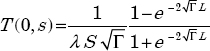
As ϕ(0,s) = 1, we obtain for H(s):

4.2.3. Frequency analysis of the diffusive phenomenon
For different values of L, the Bode diagrams presented in Figure 4.2 show that the diffusive interface:
- – behaves, in high frequency, as a fractional integrator of the order n = 0.5 (phase equal to −45°);
- – when L varies, there is a simple homothety:
- – bandwidth and static gain are changed, i.e. the modulus relative to the static gain increases with L;
- – the phase curve moves horizontally, while its amplitude remains unchanged. In particular, the amplitude of the minimum of phase is maintained.

Figure 4.2. Bode graphs of the diffusive interface: L={1 cm;5 cm;10 cm;50 cm}. For a color version of the figures in this chapter, see www.iste.co.uk/trigeassou/analysis1.zip
4.2.4. Time analysis of the diffusive phenomenon
The step responses plotted in Figure 4.3 give us a good illustration of the diffusive phenomenon: when L is small, the steady state is reached in a few seconds: it takes only 7 seconds when L = 1 cm (see Figure 4.4). Long memory is practically non-existing.
On the contrary, when L is large, the response time can be considerable: it takes more than 15000 seconds (i.e. more than 41 hours) before reaching the steady state when L = 50 cm! Therefore, transient is characterized by long memory.
The length of this memory depends on the thickness L of the wall.
REMARK 1.– The time response of the interface is obtained using the finite-difference method [FAR 82] (see also Chapter 5 Volume 2).
4.2.5. Conclusion
Frequency and time domain analysis are necessary to completely characterize the diffusive interface model. These domains are complementary:
- – The frequency domain exhibits fractional behavior, mainly the phase response at high frequencies;
- – The time response exhibits long memory behavior, mainly for large values of L corresponding to very low frequencies.

Figure 4.3. Step responses of the diffusive interface: L = {1 cm;5 cm;10 cm;50 cm}

Figure 4.4. Step response of the diffusive interface: L = 1 cm
4.3. Fractional commensurate order models
4.3.1. Physical origin
Let us consider the model of the diffusive interface given in [4.19]. By developing the exponential ![]() in series [BAT 02], we obtain:
in series [BAT 02], we obtain:
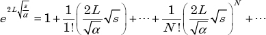
where N is an integer.
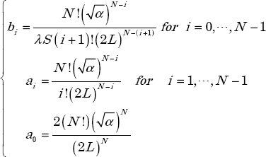
If we truncate the previous series to degree N and introduce it in (4.19), we arrive at a model HN−1,N(s) of the following form:
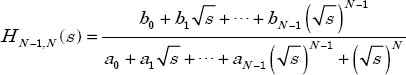
which is a commensurate order model with order n = 0.5:
with
From a mathematical point of view, truncated fractional commensurate order models are approximations of the diffusive model interface. Obviously, the quality of these approximations depends on the value of the truncation order N. A natural way to analyze these approximations is to compare their frequency responses.
4.3.2. Analysis of physical commensurate order models
Let us consider the models derived from the series truncation:
The Bode plots of the previous models and the diffusive interface are shown in Figure 4.5 for L = 1 cm and Figure 4.6 for L = 50 cm. Thus, we can note:
- – whatever the thickness L of the wall, the model H0,1(s) remains a poor approximation of H(s) , especially at low frequency. The approximation is correct only at very high frequency, i.e. when H(s) joins the fractional integrator behavior exhibiting n= 0.5 ;
- – the approximation of H(s) by H2,3(s) seems quite correct for the modulus at all frequencies. Nevertheless, the phase approximation is not correct at medium frequencies because it is not able to reproduce the minimum phase of H(s).
One way to improve the frequency approximation is to increase N: the immediate consequence would be an increase in model complexity.
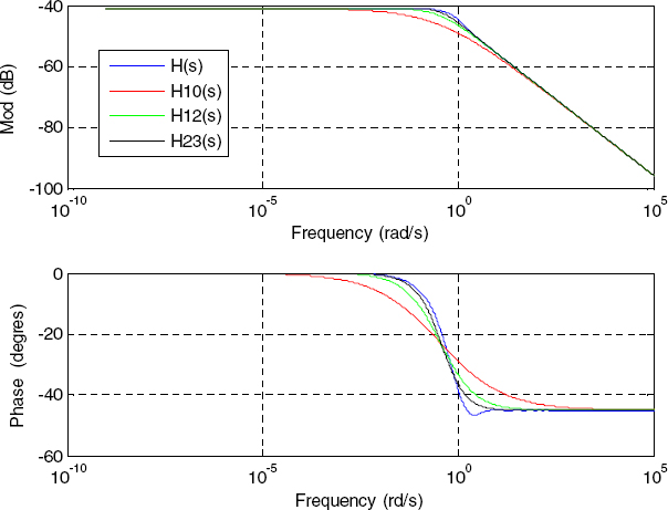
Figure 4.5. H0,1(s), H1,2(s), H2,3(s) and H(s) for L = 1 cm
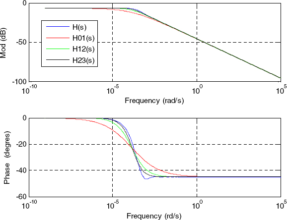
Figure 4.6. H0,1(s), H1,2(s), H2,3(s) and H(s) for L = 50 cm
4.4. Optimization of the fractional commensurate order model
4.4.1. The proposed frequency approach
We can improve the previous models ([4.24]–[4.26]) derived from the truncated series by optimizing their parameters. For this purpose, we impose the fractional commensurate order n = 0.5 , and estimate the model parameters
by minimizing a quadratic criterion.
The chosen criterion is derived from the error between the frequency response of the interface and that of the estimated model.
Because this problem is linear, it can be solved using a frequency least-squares technique [LEV 59, VAL 08] (see Appendix A.4).
Numerical examples
For L=1 cm and L=50 cm, we estimate two types of models: H0,1(s) and H2,3(s) .
For each model, two comparisons with H(s) are performed:
- – between frequency responses;
- – between step responses.
REMARK 2.– The time responses are obtained using the infinite state approach (see Chapters 2 and 3).
First, consider the H0,1(s) model (see Figures 4.7–4.10): the Bode plots show that H0,1(s) is unable to perform a good approximation of H(s) , either for L = 1 cm or L = 50 cm.
Step responses exhibit another problem. Approximations for L = 1 cm and L = 50 cm are poor and particularly H0,1(s) introduces an artifact: a non-existing long memory phenomenon appears, which is the characteristic of the one-derivative model.
Therefore, the H0,1(s) model should be rejected.
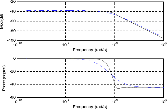
Figure 4.7. Bode diagrams with L = 1 cm: _ _ _ H 0,1(s), _____ H(s)
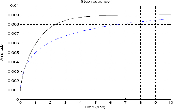
Figure 4.8. Step responses with L = 1 cm: _ _ _ H 0,1(s), _____ H(s)
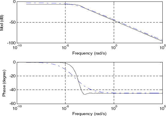
Figure 4.9. Bode diagrams with L = 50 cm: _ _ _ H 0,1(s), _____ H(s)
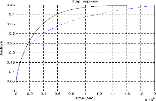
Figure 4.10. Step responses with L = 50 cm: _ _ _ H 0,1(s), _____ H(s)
On the contrary, the H2,3(s) model (see Figures 4.11–4.14) provides an excellent approximation, either for L = 1 cm or L = 50 cm. Moreover, the optimized model improves the approximations at medium frequencies (at the minimum of the phase), and provides the same step response as the true system, with the same long memory.
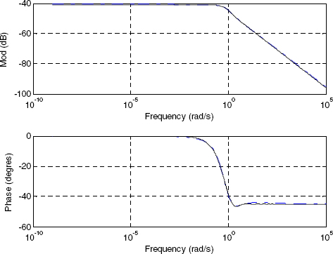
Figure 4.11. Bode diagrams with L = 1 cm: _ _ _ H2,3(s), _____ H(s)

Figure 4.12. Step responses with L = 1 cm: _ _ _ H 2,3(s), _____ H(s)
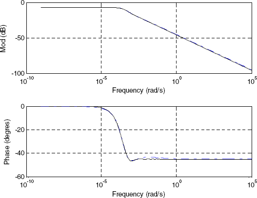
Figure 4.13. Bode diagrams with L = 50 cm: _ _ _ H 2,3(s), _____ H(s)
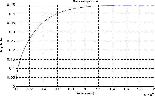
Figure 4.14. Step responses with L = 50 cm: _ _ _ H 2,3(s), _____ H(s)
4.4.2. Conclusion
The elementary model ![]() provides a poor approximation of the diffusive model interface in the time and frequency domains. Moreover, it introduces a long memory behavior which does not exist in the real system.
provides a poor approximation of the diffusive model interface in the time and frequency domains. Moreover, it introduces a long memory behavior which does not exist in the real system.
Nevertheless, the partial fraction expansion of the HN−1,N(s) model, i.e. an appropriate arrangement of H0,1(s) elementary models, provides a complex fractional commensurate order model:
which can be an excellent approximation of the diffusive model interface regardless of the thickness L (such as H2,3(s)).
Therefore, we can conclude that the elementary model H0,1(s) is only a mathematical tool, far from physics, in the case of the diffusive interface. On the contrary, the appropriate arrangement of these elementary mathematical models can be an efficient approximation of the diffusive interface, used to reproduce its time and frequency dynamics.
4.5. Fractional non-commensurate order models
4.5.1. Justification
Research works presented in [BEN 08a, JAL 12] have demonstrated that it is possible to reproduce the diffusive interface behavior through a more parsimonious model but judiciously chosen.
Let us define:
where order n1 (0 < n1 < 1) is a variable to be adjusted, whereas order n2 is imposed: n2 = 0.5.
The choice of such a model is justified by the fact that it can reproduce the high-frequency behavior (asymptotic behavior) of the diffusive interface, since:
Thus, the constraint n2 = 0.5 makes it possible to reproduce at high frequency the fractional integrator behavior of the diffusive interface.
Of course,
makes it possible to obtain the static gain.
Therefore, the non-commensurate order n1 is a supplementary parameter used to improve the frequency approximation.
4.5.2. Parameter estimation of Hn1,n2(s)
Unlike commensurate order models, we cannot derive n1 using truncation of the previous series expansion. Thus, it will be necessary to perform nonlinear parameter estimation. With the least-squares technique, the model must be linear in the parameters [LJU 87], so we cannot directly estimate the order n1.
Thus, we propose to estimate the vector:
for different values of n1 between 0 and 1 [KHA 16]. Consequently, the optimal value of n1, denoted by n1, opt, is the one that minimizes the quadratic criterion J(n1) (for more details, see Appendix A.4).
4.5.3. Numerical examples
Case L = 1 cm:
In Figure 4.15, we present the curve J(n1). Therefore, we choose n1,opt = 0.81 and the corresponding identified model. In Figures 4.16 and 4.17, the Bode diagrams and the step responses of the diffusive interface H(s) and of the model Hn1,n2(s) are compared.
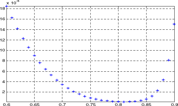
Figure 4.15. Graph J(n1) for L = 1 cm
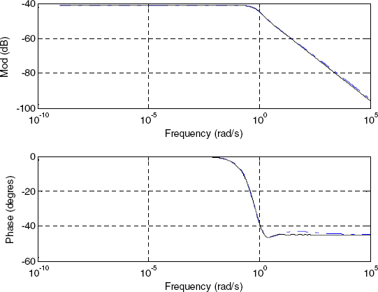
Figure 4.16. Bode diagrams with L = 1 cm: _ _ _ Hn1,n2 (s) , _____ H(s)

Figure 4.17. Step responses with L = 1 cm: _ _ _ Hn1,n2(s) , _____ H(s)
Figure 4.18, which is a zoom of Figure 4.17, shows the excellent fit between fast transients.

Figure 4.18. Transients with L = 1 cm: _ _ _ Hn1,n2(s) , _____ H(s)
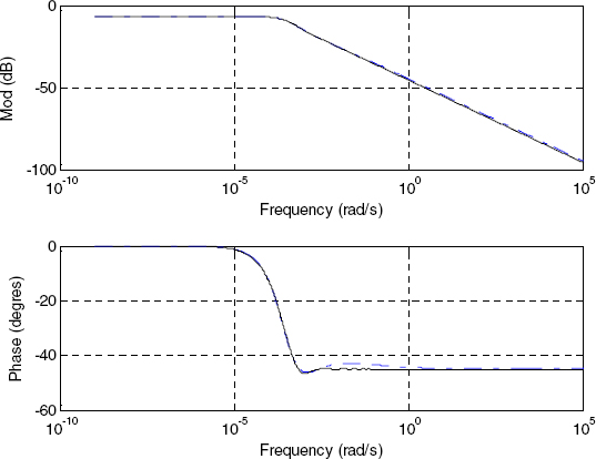
Figure 4.19. Bode diagrams with L = 50 cm: _ _ _ Hn1,n2 (s) , _____ H(s)
Case L = 50 cm:
In this case, the optimal order is n1,opt = 0.82 (close to the previous one).
We plot in Figures 4.19 and 4.20 the corresponding Bode diagrams and step responses.

Figure 4.20. Step responses with L = 50 cm: _ _ _ Hn1,n2(s) , _____ H(s)
4.5.4. Conclusion
The previous results demonstrate that the fractional non-commensurate order model Hn1,n2(s) is able to perform an excellent approximation of the diffusive interface, either in the time or frequency domain, similar to the commensurate order model H2,3(s). Of course, a more complex model Hn1,n2,n3(s) will improve this approximation. As parsimony is a fundamental requirement with fractional models, Hn1,n2(s) and H2,3(s) can be considered as optimal approximations of the diffusive interface in many practical applications.
4.6. Conclusion
Based on the prototype example of heat transfer in a plane wall, we have demonstrated that the corresponding diffusive interface model can be approximated either in the frequency or time domain by two families of fractional models: commensurate order models, where the basic order is n=0.5 , and non-commensurate order models. Moreover, the quality of the approximation can be improved with the two types of fractional models by an increase in model complexity.
An important result is that fractional models can perform an excellent approximation of physics in the case of the diffusive interface. However, simple fractional models, such as the one-derivative model, should be rejected because they provide a poor approximation of the diffusive interface as well as introduce a long memory artifact.
Of course, the identification procedures presented in this chapter cannot be used in practice because the experimental frequency response is generally not available. Therefore, the two families of fractional models should be estimated using a time identification approach (least-squares [MEN 73, LJU 87] or output error techniques [RIC 71, TRI 88]) with an appropriate excitation. Due to measurement noise, approximations performed by the H2,3(s) or Hn1,n2(s) model can be poor compared to the one provided by the H0,1(s) model. However, we should note that this elementary model is a poor approximation of physics and a generator of long memory artifact.
A.4. Appendix: estimation of frequency responses – the least-squares approach
Identification by the least-squares approach is a classical and simple technique [MEN 73]. It can be used when the model is linear in parameters: consequently, the criterion has only one minimum and the solution is analytical [LJU 87]. Moreover, it is not necessary to initialize parameter optimization as with the output error approach [RIC 01]. Its main drawback is the parameter bias caused by measurement noise [EYK 74]. Obviously, if the frequency response is exactly known, the only bias will be caused by modeling errors.
A.4.1. Identification of the commensurate order model HN−1,N(jω)
Let us define the frequency error at ωi:
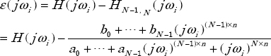
and the corresponding equation error:
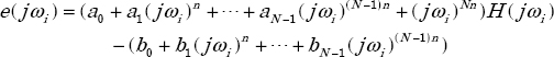
Using the parameter vector
e(jωi) can be expressed as:
with
and
Let us define the criterion to be minimized:
Thus, the optimal value of θ that minimizes J is given by [LEV 59, TRI 88, VAL 08]:
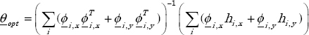
where x and y indicate respectively the real and imaginary parts.
A.4.2. Parameter estimation of the non-commensurate model 
The frequency error at ωi corresponds to:
and the corresponding equation error is:
Thus:
where n2 = 0.5 .
For a given value of n1, the parameter vector is:
Thus, en1(jωi) can be expressed as:
where
and
The quadratic criterion J(n1) corresponds to:
Then, the optimal value of θ is given by:
The quality of the obtained models depends on the choice of the pulsations ωi which have to be chosen in the vicinity of the phase minimum of H(jω). Moreover, their distribution must be logarithmic.