1.1 Asset Returns

Most financial studies involve returns, instead of prices, of assets. Campbell, Lo, and MacKinlay (1997) give two main reasons for using returns. First, for average investors, return of an asset is a complete and scale-free summary of the investment opportunity. Second, return series are easier to handle than price series because the former have more attractive statistical properties. There are, however, several definitions of an asset return.

Let Pt be the price of an asset at time index t. We discuss some definitions of returns that are used throughout the book. Assume for the moment that the asset pays no dividends.

One-Period Simple Return

Holding the asset for one period from date t − 1 to date t would result in a simple gross return:

1.1

The corresponding one-period simple net return or simple return is

1.2

Multiperiod Simple Return

Holding the asset for k periods between dates t − k and t gives a k-period simple gross return:

Thus, the k-period simple gross return is just the product of the k one-period simple gross returns involved. This is called a compound return. The k-period simple net return is Rt[k] = (Pt − Pt−k)/Pt−k.

In practice, the actual time interval is important in discussing and comparing returns (e.g., monthly return or annual return). If the time interval is not given, then it is implicitly assumed to be one year. If the asset was held for k years, then the annualized (average) return is defined as

This is a geometric mean of the k one-period simple gross returns involved and can be computed by

where exp(x) denotes the exponential function and ln(x) is the natural logarithm of the positive number x. Because it is easier to compute arithmetic average than geometric mean and the one-period returns tend to be small, one can use a first-order Taylor expansion to approximate the annualized return and obtain

1.3

Accuracy of the approximation in Eq. (1.3) may not be sufficient in some applications, however.

Continuous Compounding

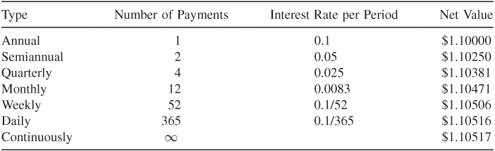
Before introducing continuously compounded return, we discuss the effect of compounding. Assume that the interest rate of a bank deposit is 10% per annum and the initial deposit is $1.00. If the bank pays interest once a year, then the net value of the deposit becomes $1(1 + 0.1) = $1.1 one year later. If the bank pays interest semiannually, the 6-month interest rate is 10%/2 = 5% and the net value is $1(1 + 0.1/2)2 = $1.1025 after the first year. In general, if the bank pays interest m times a year, then the interest rate for each payment is 10%/m and the net value of the deposit becomes $1(1 + 0.1/m)m one year later. Table 1.1 gives the results for some commonly used time intervals on a deposit of $1.00 with interest rate of 10% per annum. In particular, the net value approaches $1.1052, which is obtained by exp(0.1) and referred to as the result of continuous compounding. The effect of compounding is clearly seen.

Table 1.1 Illustration of Effects of Compounding: Time Interval Is 1 Year and Interest Rate Is 10% per Annum

In general, the net asset value A of continuous compounding is

1.4

where r is the interest rate per annum, C is the initial capital, and n is the number of years. From Eq. (1.4), we have

1.5

which is referred to as the present value of an asset that is worth A dollars n years from now, assuming that the continuously compounded interest rate is r per annum.

Continuously Compounded Return

The natural logarithm of the simple gross return of an asset is called the continuously compounded return or log return:

1.6

where pt = ln(Pt). Continuously compounded returns rt enjoy some advantages over the simple net returns Rt. First, consider multiperiod returns. We have

Thus, the continuously compounded multiperiod return is simply the sum of continuously compounded one-period returns involved. Second, statistical properties of log returns are more tractable.

Portfolio Return

The simple net return of a portfolio consisting of N assets is a weighted average of the simple net returns of the assets involved, where the weight on each asset is the percentage of the portfolio's value invested in that asset. Let p be a portfolio that places weight wi on asset i. Then the simple return of p at time t is , where Rit is the simple return of asset i.

The continuously compounded returns of a portfolio, however, do not have the above convenient property. If the simple returns Rit are all small in magnitude, then we have , where rp,t is the continuously compounded return of the portfolio at time t. This approximation is often used to study portfolio returns.

Dividend Payment

If an asset pays dividends periodically, we must modify the definitions of asset returns. Let Dt be the dividend payment of an asset between dates t − 1 and t and Pt be the price of the asset at the end of period t. Thus, dividend is not included in Pt. Then the simple net return and continuously compounded return at time t become

Excess Return

Excess return of an asset at time t is the difference between the asset's return and the return on some reference asset. The reference asset is often taken to be riskless such as a short-term U.S. Treasury bill return. The simple excess return and log excess return of an asset are then defined as

1.7

where R0t and r0t are the simple and log returns of the reference asset, respectively. In the finance literature, the excess return is thought of as the payoff on an arbitrage portfolio that goes long in an asset and short in the reference asset with no net initial investment.

Summary of Relationship

The relationships between simple return Rt and continuously compounded (or log) return rt are

If the returns Rt and rt are in percentages, then

Temporal aggregation of the returns produces

If the continuously compounded interest rate is r per annum, then the relationship between present and future values of an asset is