11.4 Kalman Filter and Smoothing

In this section, we study the Kalman filter and various smoothing methods for the general state-space model in Eqs. (11.26) and (11.27). The derivation follows closely the steps taken in Section 11.1. For readers interested in applications, this section can be skipped at the first read. A good reference for this section is Durbin and Koopman (2001, Chapter 4).

11.4.1 Kalman Filter

Recall that the aim of the Kalman filter is to obtain recursively the conditional distribution of st+1 given the data Ft = {yt, …, yt} and the model. Since the conditional distribution involved is normal, it suffices to study the conditional mean and covariance matrix. Let st+1 and ∑jIi be the conditional mean and covariance matrix of st given Fi, that is, sj I Fi ~ Ni(sjIi, ∑jIi) From Eq. (11.26),

11.55

11.56

Similarly to that of Section 11.1, let ytIt-1 be the conditional mean of yt given Ft−1. From Eq. (11.27),

Let

11.57

be the 1-step-ahead forecast error of yt given Ft−1. It is easy to see that (a) E(vtIFt-1 = 0; (b) ut is independent of Ft−1, that is, Cov(vtyt) = 0 for 1 ≤ j < t; and (c) {vt} is a sequence of independent normal random vectors. Also, let Vt = Var(vtIFt-1 be the covariance matrix of the 1-step-ahead forecast error. From Eq. (11.57), we have

11.58

Since Ft = {Ft-1, yt}, = {Ft-1, vt} we can apply Theorem 11.1 to obtain

11.59

where Ft = {Ft-1, yt} = {Ft-1, vt} given by

Here we assume that Vt is invertible because Ht is. Using Eqs. (11.55) and (11.59), we obtain

11.60

where

11.61

which is the Kalman gain at time t. Applying Theorem 11.1(2), we have

11.62

Plugging Eq. (11.62) into Eq. (11.56) and using Eq. (11.61), we obtain

11.63

where

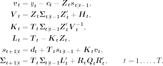
Putting the prior equations together, we obtain the celebrated Kalman filter for the state-space model in Eqs. (11.26) and (11.27). Given the starting values s1I0 and ∑1I0, the Kalman filter algorithm is

11.64

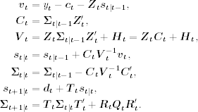
If the filtered quantities s1It and ∑1It are also of interest, then we modify the filter to include the contemporaneous filtering equations in Eqs. (11.59) and (11.62). The resulting algorithm is

Steady State

If the state-space model is time invariant, that is, all system matrices are time invariant, then the matrices ∑tIt-1 converge to a constant matrix ∑٭, which is a solution of the matrix equation

where V = Z∑٭Z′+H. The solution that is reached after convergence to ∑٭ is referred to as the steady-state solution of the Kalman filter. Once the steady state is reached, Vt, Kt, and Kt+1It are all constant. This can lead to considerable saving in computing time.

11.4.2 State Estimation Error and Forecast Error

Define the state prediction error as

From the definition, the covariance matrix of xt is Var(xtIFt-1) = Var(stIFt-1) = ∑tIt-1. Following Section 11.1, we investigate properties of xt . First, from Eq. (11.57),

Second, from Eqs. (11.64) and (11.26), and the prior equation, we have

where, as before, Lt = Tt - KtZt. Consequently, we obtain a state-space form for vt as

11.65

with x1 = st for 1 - s1It = 1, … , T.

Finally, similar to the local-trend model in Section 11.1, we can show that the 1-step-ahead forecast errors {vt} are independent of each other and {vt, …, vT} is independent of Ft−1.

11.4.3 State Smoothing

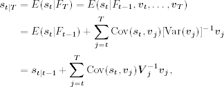
State smoothing focuses on the conditional distribution of st given FT. Notice that (a) Ft−1 and {vt, …, vT} are independent and (b) vt are serially independent. We can apply Theorem 11.1 to the joint distribution of st and {vt, …, vT} given Ft−1 and obtain

11.66

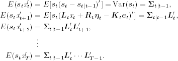
where the covariance matrices are conditional on Ft−1. The covariance matrices Cov(st, vj) for j = t, … , T can be derived as follows. By Eq. (11.65),

11.67

Furthermore,

11.68

Plugging the prior two equations into Eq. (11.66), we have

for t = T − 2, T − 3, … , 1, where it is understood that = Tn when t = T. These smoothed state vectors can be expressed as

11.69

where, and

for t = T − 2, T − 3, … , 1. The quantity qt-1 is a weighted sum of the 1-step-ahead forecast errors vj occurring after time t − 1. From the definition in the prior equation, qt can be computed recursively backward as

11.70

with qT = 0. Putting the equations together, we have a backward recursion for the smoothed state vectors as

11.71

starting with qt = 0, where stIT, ∑tIt-1, Lt and Vt are available from the Kalman filter. This algorithm is referred to as the fixed interval smoother in the literature; see de Jong (1989) and the references therein.

Covariance Matrix of Smoothed State Vector

Next, we derive the covariance matrices of the smoothed state vectors. Applying Theorem 11.1(4) to the conditional joint distribution of st and {vt, …, vT} given Ft−1, we have

Using the covariance matrices in Eqs. (11.67) and (11.68), we further obtain

where

Again, when t = T. From its definition, the Mt-1 matrix satisfies

11.72

with the starting value MT = 0. Collecting the results, we obtain a backward recursion to compute ∑tIT as

11.73

for t = T, … , 1 with Mt-1 = 0. Note that, like that of the local trend model in Section 11.1, Mt = Var(qt).

Combining the two backward recursions of smoothed state vectors, we have

11.74

with qt = 0 and MT = 0.

Suppose that the state-space model in Eqs. (11.26) and (11.27) is known. Application of the Kalman filter and state smoothing can proceed in two steps. First, the Kalman filter in Eq. (11.64) is used for t = 1, … , T and the quantities vt,Vt, Kt, stIt-1, and ∑tIt-1 are stored. Second, the state smoothing algorithm in Eq. (11.74) is applied for t = T, T − 1, … , 1 to obtain stIT and ∑tIT.

11.4.4 Disturbance Smoothing

Let etIT = E(etI Ft) and ηtIT = E(ηtI Ft) be the smoothed disturbances of the observation and transition equation, respectively. These smoothed disturbances are useful in many applications, for example, in model checking. In this section, we study recursive algorithms to compute smoothed disturbances and their covariance matrices. Again, applying Theorem 11.1 to the conditional joint distribution of et and {vt, …, vt} given Ft−1, we obtain

11.75

where E(etIFt) = 0 is used. Using Eq. (11.65),

Since , we have

11.76

Using Eq. (11.65) repeatedly and the independence between {et} and {ηt}, we obtain

11.77

where it is understood that = Im if t = T − 1. Based on Eqs. (11.76) and (11.77),

11.78

where qt is defined in Eq. (11.69) and . We refer to ot as the smoothing measurement error.

The smoothed disturbance ηtIT can be derived analogously, and we have

11.79

The state-space form in Eq. (11.69) gives

where

for t = 1, … , T. Consequently, Eq. (11.79) implies

11.80

where qt is defined earlier in Eq. (11.70).

Koopman (1993) uses the smoothed disturbance ηtIT to derive a new recursion for computing stIT. From the transition equation in Eq. (11.26),

Using Eq. (11.80), we have

11.81

where the initial value is stIT = s1I0 + ∑tI0q0 with q obtained from the recursion in Eq. (11.70).

Covariance Matrices of Smoothed Disturbances

The covariance matrix of the smoothed disturbance can also be obtained using Theorem 11.1. Specifically,

Note that , which is given in Eq. (11.76). Thus, we have

where , where Mt is given in Eq. (11.72). Similarly,

where Cov(ηt, vt) = , which is given before when we derived the formula for ηtIT. Consequently,

In summary, the disturbance smoothing algorithm is as follows:

11.82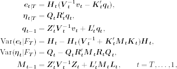

where qT = 0 and MT = 0.