
We now turn to another class of simple models that are also useful in modeling return series in finance. These models are the moving-average (MA) models. As is shown in Chapter 5, the bid–ask bounce in stock trading may introduce an MA(1) structure in a return series. There are several ways to introduce MA models. One approach is to treat the model as a simple extension of white noise series. Another approach is to treat the model as an infinite-order AR model with some parameter constraints. We adopt the second approach.
There is no particular reason, but simplicity, to assume a priori that the order of an AR model is finite. We may entertain, at least in theory, an AR model with infinite order as
![]()
However, such an AR model is not realistic because it has infinite many parameters. One way to make the model practical is to assume that the coefficients ϕi's satisfy some constraints so that they are determined by a finite number of parameters. A special case of this idea is
where the coefficients depend on a single parameter θ1 via ![]() for i ≥ 1. For the model in Eq. (2.17) to be stationary, θ1 must be less than 1 in absolute value; otherwise,
for i ≥ 1. For the model in Eq. (2.17) to be stationary, θ1 must be less than 1 in absolute value; otherwise, ![]() and the series will explode. Because |θ1| < 1, we have
and the series will explode. Because |θ1| < 1, we have ![]() as i → ∞. Thus, the contribution of rt−i to rt decays exponentially as i increases. This is reasonable as the dependence of a stationary series rt on its lagged value rt−i, if any, should decay over time.
as i → ∞. Thus, the contribution of rt−i to rt decays exponentially as i increases. This is reasonable as the dependence of a stationary series rt on its lagged value rt−i, if any, should decay over time.
The model in Eq. (2.17) can be rewritten in a rather compact form. To see this, rewrite the model as
The model for rt−1 is then
Multiplying Eq. (2.19) by θ1 and subtracting the result from Eq. (2.18), we obtain
![]()
which says that except for the constant term rt is a weighted average of shocks at and at−1. Therefore, the model is called an MA model of order 1 or MA(1) model for short. The general form of an MA(1) model is
where c0 is a constant and {at} is a white noise series. Similarly, an MA(2) model is in the form
and an MA(q) model is
or rt = c0 + (1 − θ1B − ⋯ − θqBq)at, where q > 0.
2.5.1 Properties of MA Models
Again, we focus on the simple MA(1) and MA(2) models. The results of MA(q) models can easily be obtained by the same techniques.
Stationarity
Moving-average models are always weakly stationary because they are finite linear combinations of a white noise sequence for which the first two moments are time invariant. For example, consider the MA(1) model in Eq. (2.20). Taking expectation of the model, we have
![]()
which is time invariant. Taking the variance of Eq. (2.20), we have
![]()
where we use the fact that at and at−1 are uncorrelated. Again, Var(rt) is time invariant. The prior discussion applies to general MA(q) models, and we obtain two general properties. First, the constant term of an MA model is the mean of the series [i.e., E(rt) = c0]. Second, the variance of an MA(q) model is
![]()
Autocorrelation Function
Assume for simplicity that c0 = 0 for an MA(1) model. Multiplying the model by rt−ℓ, we have
![]()
Taking expectation, we obtain
![]()
Using the prior result and the fact that Var(rt) = ![]() , we have
, we have
![]()
Thus, for an MA(1) model, the lag-1 ACF is not zero, but all higher order ACFs are zero. In other words, the ACF of an MA(1) model cuts off at lag 1. For the MA(2) model in Eq. (2.21), the autocorrelation coefficients are
![]()
Here the ACF cuts off at lag 2. This property generalizes to other MA models. For an MA(q) model, the lag-q ACF is not zero, but ρℓ = 0 for ℓ > q. Consequently, an MA(q) series is only linearly related to its first q-lagged values and hence is a “finite-memory” model.
Invertibility
Rewriting a zero-mean MA(1) model as at = rt + θ1at−1, one can use repeated substitutions to obtain
![]()
This equation expresses the current shock at as a linear combination of the present and past returns. Intuitively, ![]() should go to zero as j increases because the remote return rt−j should have very little impact on the current shock, if any. Consequently, for an MA(1) model to be plausible, we require |θ1| < 1. Such an MA(1) model is said to be invertible. If |θ1| = 1, then the MA(1) model is noninvertible. See Section 2.6.5 for further discussion on invertibility.
should go to zero as j increases because the remote return rt−j should have very little impact on the current shock, if any. Consequently, for an MA(1) model to be plausible, we require |θ1| < 1. Such an MA(1) model is said to be invertible. If |θ1| = 1, then the MA(1) model is noninvertible. See Section 2.6.5 for further discussion on invertibility.
2.5.2 Identifying MA Order
The ACF is useful in identifying the order of an MA model. For a time series rt with ACF ρℓ, if ρq ≠ 0, but ρℓ = 0 for ℓ > q, then rt follows an MA(q) model.
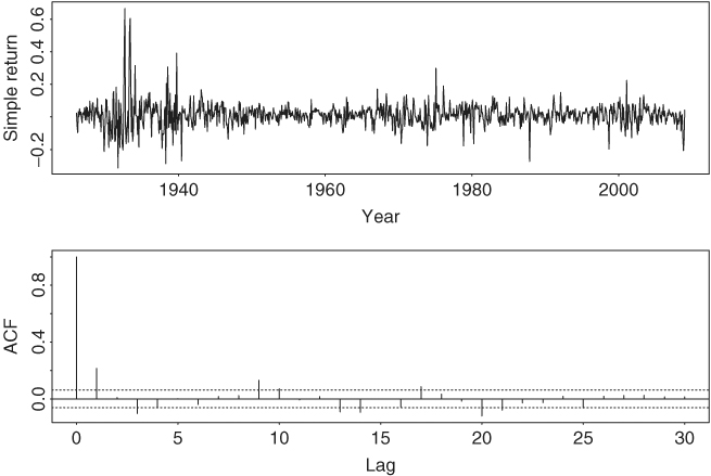
Figure 2.8 shows the time plot of monthly simple returns of the CRSP equal-weighted index from January 1926 to December 2008 and the sample ACF of the series. The two dashed lines shown on the ACF plot denote the two standard error limits. It is seen that the series has significant ACF at lags 1, 3, and 9. There are some marginally significant ACF at higher lags, but we do not consider them here. Based on the sample ACF, the following MA(9) model
![]()
is identified for the series. Note that, unlike the sample PACF, sample ACF provides information on the nonzero MA lags of the model.
Figure 2.8 Time plot and sample autocorrelation function of monthly simple returns of CRSP equal-weighted index from January 1926 to December 2008.
2.5.3 Estimation
Maximum-likelihood estimation is commonly used to estimate MA models. There are two approaches for evaluating the likelihood function of an MA model. The first approach assumes that the initial shocks (i.e., at for t ≤ 0) are zero. As such, the shocks needed in likelihood function calculation are obtained recursively from the model, starting with a1 = r1 − c0 and a2 = r2 − c0 + θ1a1. This approach is referred to as the conditional-likelihood method and the resulting estimates the conditional maximum-likelihood estimates. The second approach treats the initial shocks at, t ≤ 0, as additional parameters of the model and estimate them jointly with other parameters. This approach is referred to as the exact-likelihood method. The exact-likelihood estimates are preferred over the conditional ones, especially when the MA model is close to being noninvertible. The exact method, however, requires more intensive computation. If the sample size is large, then the two types of maximum-likelihood estimates are close to each other. For details of conditional- and exact-likelihood estimates of MA models, readers are referred to Box, Jenkins, and Reinsel (1994) or Chapter 8.
For illustration, consider the monthly simple return series of the CRSP equal-weighted index and the specified MA(9) model. The conditional maximum-likelihood method produces the fitted model
where standard errors of the coefficient estimates are 0.003, 0.031, 0.031, and 0.031, respectively. The Ljung–Box statistics of the residuals give Q(12) = 17.5 with a p value 0.041, which is based on an asymptotic chi-squared distribution with 9 degrees of freedom. The model needs some refinements in modeling the linear dynamic dependence of the data. The p value would be 0.132 if 12 degrees of freedom are used. The exact maximum-likelihood method produces the fitted model
where standard errors of the estimates are 0.003, 0.031, 0.031, and 0.031, respectively. The Ljung–Box statistics of the residuals give Q(12) = 17.6. The corresponding p values are 0.040 and 0.128, respectively, when the degrees of freedom are 9 and 12. Again, this fitted model is only marginally adequate. Comparing models (2.23) and (2.24), we see that for this particular instance, the difference between the conditional- and exact-likelihood methods is negligible.
2.5.4 Forecasting Using MA Models
Forecasts of an MA model can easily be obtained. Because the model has finite memory, its point forecasts go to the mean of the series quickly. To see this, assume that the forecast origin is h and let Fh denote the information available at time h. For the 1-step-ahead forecast of an MA(1) process, the model says
![]()
Taking the conditional expectation, we have
![]()
The variance of the 1-step-ahead forecast error is Var[eh(1)] = ![]() . In practice, the quantity ah can be obtained in several ways. For instance, assume that a0 = 0, then a1 = r1 − c0, and we can compute at for 2 ≤ t ≤ h recursively by using at = rt − c0 + θ1at−1. Alternatively, it can be computed by using the AR representation of the MA(1) model; see Section 2.6.5. Of course, at is the residual series of a fitted MA(1) model. Thus, ah is readily available from the estimation.
. In practice, the quantity ah can be obtained in several ways. For instance, assume that a0 = 0, then a1 = r1 − c0, and we can compute at for 2 ≤ t ≤ h recursively by using at = rt − c0 + θ1at−1. Alternatively, it can be computed by using the AR representation of the MA(1) model; see Section 2.6.5. Of course, at is the residual series of a fitted MA(1) model. Thus, ah is readily available from the estimation.
For the 2-step-ahead forecast from the equation
![]()
we have
![]()
The variance of the forecast error is Var![]() , which is the variance of the model and is greater than or equal to that of the 1-step-ahead forecast error. The prior result shows that for an MA(1) model the 2-step-ahead forecast of the series is simply the unconditional mean of the model. This is true for any forecast origin h. More generally,
, which is the variance of the model and is greater than or equal to that of the 1-step-ahead forecast error. The prior result shows that for an MA(1) model the 2-step-ahead forecast of the series is simply the unconditional mean of the model. This is true for any forecast origin h. More generally, ![]() for ℓ ≥ 2. In summary, for an MA(1) model, the 1-step-ahead point forecast at the forecast origin h is c0 − θ1ah and the multistep ahead forecasts are c0, which is the unconditional mean of the model. If we plot the forecasts
for ℓ ≥ 2. In summary, for an MA(1) model, the 1-step-ahead point forecast at the forecast origin h is c0 − θ1ah and the multistep ahead forecasts are c0, which is the unconditional mean of the model. If we plot the forecasts ![]() versus ℓ, we see that the forecasts form a horizontal line after one step. Thus, for MA(1) models, mean reverting only takes one time period.
versus ℓ, we see that the forecasts form a horizontal line after one step. Thus, for MA(1) models, mean reverting only takes one time period.
Similarly, for an MA(2) model, we have
![]()
from which we obtain
Thus, the multistep-ahead forecasts of an MA(2) model go to the mean of the series after two steps. The variances of forecast errors go to the variance of the series after two steps. In general, for an MA(q) model, multistep-ahead forecasts go to the mean after the first q steps.
Table 2.3 gives some out-of-sample forecasts of an MA(9) model in the form of Eq. (2.24) for the monthly simple returns of the equal-weighted index at the forecast origin h = 986 (February 2008). The model parameters are reestimated using the first 986 observations. The sample mean and standard error of the estimation subsample are 0.0128 and 0.0736, respectively. As expected, the table shows that (a) the 10-step-ahead forecast is the sample mean, and (b) the standard deviations of the forecast errors converge to the standard deviation of the series as the forecast horizon increases. In this particular case, the point forecasts deviate substantially from the observed returns because of the worldwide financial crisis caused by the subprime mortgage problem and the collapse of Lehman Brothers.
Table 2.3 Out-of-Sample Forecast Performance of an MA(9) Model for Monthly Simple Returns of CRSP Equal-Weighted Indexa
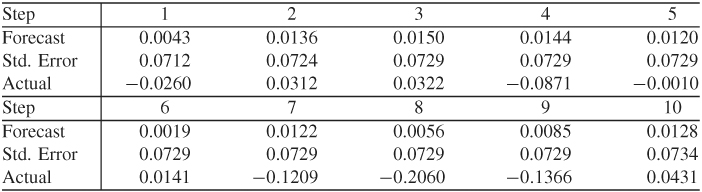
aThe forecast origin is February 2008 With h = 986. The model is estimated by the exact maximum-likelihood method.
Summary
A brief summary of AR and MA models is in order. We have discussed the following properties:
- For MA models, ACF is useful in specifying the order because ACF cuts off at lag q for an MA(q) series.
- For AR models, PACF is useful in order determination because PACF cuts off at lag p for an AR(p) process.
- An MA series is always stationary, but for an AR series to be stationary, all of its characteristic roots must be less than 1 in modulus.
- For a stationary series, the multistep-ahead forecasts converge to the mean of the series, and the variances of forecast errors converge to the variance of the series as the forecast horizon increases.