
9.4 Principal Component Analysis
An important topic in multivariate time series analysis is the study of the covariance (or correlation) structure of the series. For example, the covariance structure of a vector return series plays an important role in portfolio selection. In what follows, we discuss some statistical methods useful in studying the covariance structure of a vector time series.
Given a k-dimensional random variable ![]() with covariance matrix
with covariance matrix ![]() , a principal component analysis (PCA) is concerned with using a few linear combinations of ri to explain the structure of
, a principal component analysis (PCA) is concerned with using a few linear combinations of ri to explain the structure of ![]() . If
. If ![]() denotes the monthly log returns of k assets, then PCA can be used to study the main source of variations of these k asset returns. Here the keyword is few so that simplification can be achieved in multivariate analysis.
denotes the monthly log returns of k assets, then PCA can be used to study the main source of variations of these k asset returns. Here the keyword is few so that simplification can be achieved in multivariate analysis.
9.4.1 Theory of PCA
Principal component analysis applies to either the covariance matrix ![]() or the correlation matrix
or the correlation matrix ![]() of
of ![]() . Since the correlation matrix is the covariance matrix of the standardized random vector
. Since the correlation matrix is the covariance matrix of the standardized random vector ![]() , where
, where ![]() is the diagonal matrix of standard deviations of the components of
is the diagonal matrix of standard deviations of the components of ![]() , we use covariance matrix in our theoretical discussion. Let
, we use covariance matrix in our theoretical discussion. Let ![]() be a k-dimensional real-valued vector, where i = 1, … , k. Then
be a k-dimensional real-valued vector, where i = 1, … , k. Then
![]()
is a linear combination of the random vector ![]() . If
. If ![]() consists of the simple returns of k stocks, then yi is the return of a portfolio that assigns weight wij to the jth stock. Since multiplying a constant to
consists of the simple returns of k stocks, then yi is the return of a portfolio that assigns weight wij to the jth stock. Since multiplying a constant to ![]() does not affect the proportion of allocation assigned to the jth stock, we standardize the vector
does not affect the proportion of allocation assigned to the jth stock, we standardize the vector ![]() so that
so that ![]() =
=![]() .
.
Using properties of a linear combination of random variables, we have
9.11 ![]()
9.12 ![]()
The idea of PCA is to find linear combinations ![]() such that yi and yj are uncorrelated for i ≠ j and the variances of yi are as large as possible. More specifically:
such that yi and yj are uncorrelated for i ≠ j and the variances of yi are as large as possible. More specifically:
1. The first principal component of ![]() is the linear combination
is the linear combination ![]() that maximizes Var(y1) subject to the constraint
that maximizes Var(y1) subject to the constraint ![]() = 1.
= 1.
2. The second principal component of ![]() is the linear combination
is the linear combination ![]() that maximizes Var(y2) subject to the constraints
that maximizes Var(y2) subject to the constraints ![]() = 1 and Cov(y2, y1) = 0.
= 1 and Cov(y2, y1) = 0.
3. The ith principal component of ![]() is the linear combination
is the linear combination ![]() that maximizes Var(yi) subject to the constraints
that maximizes Var(yi) subject to the constraints ![]() = 1 and Cov(yi, yj) = 0 for j = 1, … , i − 1.
= 1 and Cov(yi, yj) = 0 for j = 1, … , i − 1.
Since the covariance matrix ![]() is nonnegative definite, it has a spectral decomposition; see Appendix A of Chapter 8. Let
is nonnegative definite, it has a spectral decomposition; see Appendix A of Chapter 8. Let ![]() , …,
, …, ![]() be the eigenvalue–eigenvector pairs of
be the eigenvalue–eigenvector pairs of ![]() , where λ1 ≥ λ2 ≥ ⋯ ≥ λk ≥ 0 and
, where λ1 ≥ λ2 ≥ ⋯ ≥ λk ≥ 0 and ![]() , which is properly normalized. We have the following statistical result.
, which is properly normalized. We have the following statistical result.
Result 9.1
The ith principal component of ![]() is
is ![]() =
= ![]() for i = 1, … , k. Moreover,
for i = 1, … , k. Moreover,
![]()
If some eigenvalues λi are equal, the choices of the corresponding eigenvectors ![]() and hence yi are not unique. In addition, we have
and hence yi are not unique. In addition, we have
The result of Eq. (9.13) says that
![]()
Consequently, the proportion of total variance in ![]() explained by the ith principal component is simply the ratio between the ith eigenvalue and the sum of all eigenvalues of
explained by the ith principal component is simply the ratio between the ith eigenvalue and the sum of all eigenvalues of ![]() . One can also compute the cumulative proportion of total variance explained by the first i principal components [i.e.,
. One can also compute the cumulative proportion of total variance explained by the first i principal components [i.e., ![]() ]. In practice, one selects a small i such that the resulting cumulative proportion is large.
]. In practice, one selects a small i such that the resulting cumulative proportion is large.
Since ![]() = k, the proportion of variance explained by the ith principal component becomes λi/k when the correlation matrix is used to perform the PCA.
= k, the proportion of variance explained by the ith principal component becomes λi/k when the correlation matrix is used to perform the PCA.
A by-product of the PCA is that a zero eigenvalue of ![]() , or
, or ![]() , indicates the existence of an exact linear relationship between the components of
, indicates the existence of an exact linear relationship between the components of ![]() . For instance, if the smallest eigenvalue λk = 0, then by Result 9.1 Var(yk) = 0. Therefore, yk =
. For instance, if the smallest eigenvalue λk = 0, then by Result 9.1 Var(yk) = 0. Therefore, yk = ![]() is a constant and there are only k − 1 random quantities in
is a constant and there are only k − 1 random quantities in ![]() . In this case, the dimension of
. In this case, the dimension of ![]() can be reduced. For this reason, PCA has been used in the literature as a tool for dimension reduction.
can be reduced. For this reason, PCA has been used in the literature as a tool for dimension reduction.
9.4.2 Empirical PCA
In application, the covariance matrix ![]() and the correlation matrix
and the correlation matrix ![]() of the return vector
of the return vector ![]() are unknown, but they can be estimated consistently by the sample covariance and correlation matrices under some regularity conditions. Assuming that the returns are weakly stationary and the data consist of
are unknown, but they can be estimated consistently by the sample covariance and correlation matrices under some regularity conditions. Assuming that the returns are weakly stationary and the data consist of ![]() , we have the following estimates:
, we have the following estimates:
9.14 ![]()
9.15 ![]()
where ![]() = diag
= diag![]() is the diagonal matrix of sample standard errors of
is the diagonal matrix of sample standard errors of ![]() . Methods to compute eigenvalues and eigenvectors of a symmetric matrix can then be used to perform the PCA. Most statistical packages now have the capability to perform principal component analysis. In R and S-Plus, the basic command of PCA is princomp, and in FinMetrics the command is mfactor.
. Methods to compute eigenvalues and eigenvectors of a symmetric matrix can then be used to perform the PCA. Most statistical packages now have the capability to perform principal component analysis. In R and S-Plus, the basic command of PCA is princomp, and in FinMetrics the command is mfactor.
Example 9.1
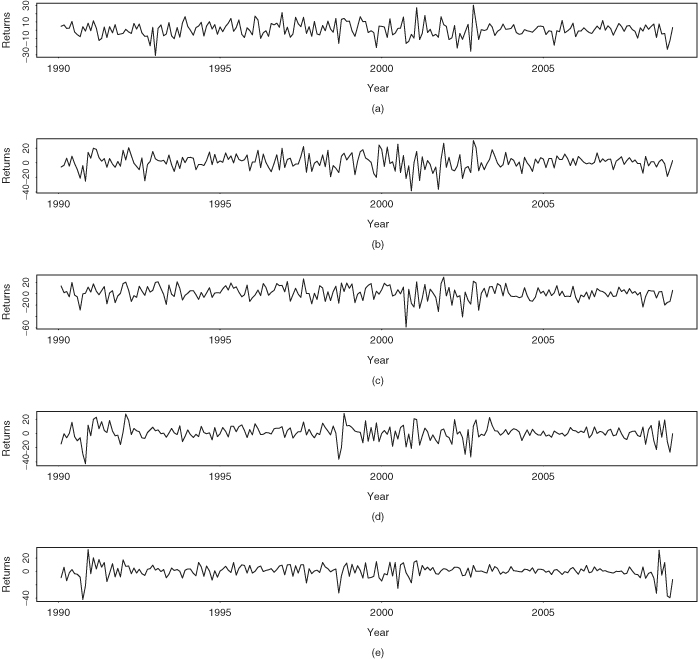
Consider the monthly log stock returns of International Business Machines, Hewlett-Packard, Intel Corporation, J.P. Morgan Chase, and Bank of America from January 1990 to December 2008. The returns are in percentages and include dividends. The data set has 228 observations. Figure 9.4 shows the time plots of these five monthly return series. As expected, returns of companies in the same industrial sector tend to exhibit similar patterns.
Figure 9.4 Time plots of monthly log stock returns in percentages and including dividends for (a) International Business Machines, (b) Hewlett-Packard, (c) Intel, (d) J.P. Morgan Chase, and (e) Bank of America from January 1990 to December 2008.
Denote the returns by ![]() = (IBM, HPQ, INTC, JPM, BAC). The sample mean vector of the returns is (0.70, 0.99, 1.20, 0.82, 0.41)′ and the sample covariance and correlation matrices are
= (IBM, HPQ, INTC, JPM, BAC). The sample mean vector of the returns is (0.70, 0.99, 1.20, 0.82, 0.41)′ and the sample covariance and correlation matrices are
Table 9.3 gives the results of PCA using both the covariance and correlation matrices. Also given are eigenvalues, eigenvectors, and proportions of variabilities explained by the principal components. Consider the correlation matrix and denote the sample eigenvalues and eigenvectors by ![]() and
and ![]() . We have
. We have
![]()
for the first two principal components. These two components explain about 74% of the total variability of the data, and they have interesting interpretations. The first component is a roughly equally weighted linear combination of the stock returns. This component might represent the general movement of the stock market and hence is a market component. The second component represents the difference between the two industrial sectors—namely, technologies versus financial services. It might be an industrial component. Similar interpretations of principal components can also be found by using the covariance matrix of ![]() .
.
Table 9.3 Results of Principal Component Analysis for Monthly Log Returns, Including Dividends of Stocks of IBM, Hewlett-Packard, Intel, J.P. Morgan Chase, and Bank of America from January 1990 to December 2008a
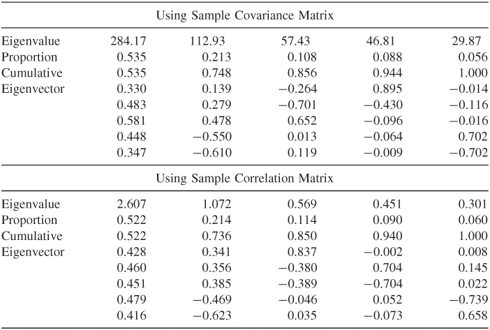
aThe eigenvectors are in columns.
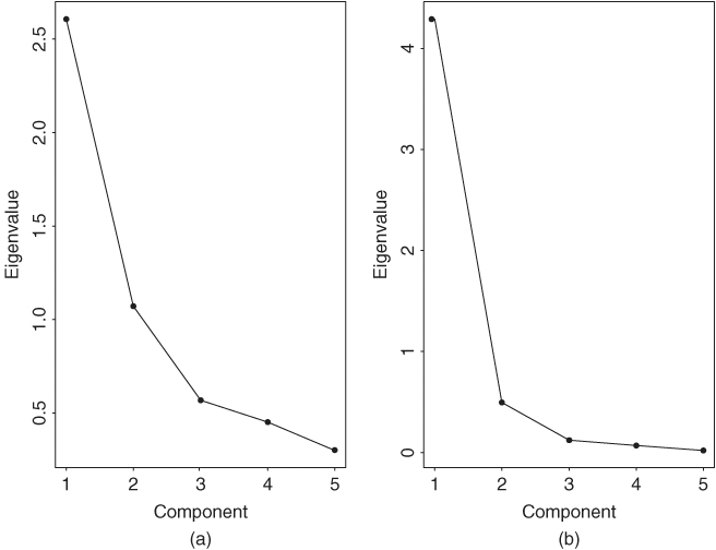
An informal but useful procedure to determine the number of principal components needed in an application is to examine the scree plot, which is the time plot of the eigenvalues ![]() ordered from the largest to the smallest (i.e., a plot of
ordered from the largest to the smallest (i.e., a plot of ![]() versus i). Figure 9.5(a) shows the scree plot for the five stock returns of Example 9.1. By looking for an elbow in the scree plot, indicating that the remaining eigenvalues are relatively small and all about the same size, one can determine the appropriate number of components. For both plots in Figure 9.5, two components appear to be appropriate. Finally, except for the case in which λj = 0 for j > i, selecting the first i principal components only provides an approximation to the total variance of the data. If a small i can provide a good approximation, then the simplification becomes valuable.
versus i). Figure 9.5(a) shows the scree plot for the five stock returns of Example 9.1. By looking for an elbow in the scree plot, indicating that the remaining eigenvalues are relatively small and all about the same size, one can determine the appropriate number of components. For both plots in Figure 9.5, two components appear to be appropriate. Finally, except for the case in which λj = 0 for j > i, selecting the first i principal components only provides an approximation to the total variance of the data. If a small i can provide a good approximation, then the simplification becomes valuable.
Remark
The R and S-Plus commands used to perform the PCA are given below. The command princomp gives the square root of the eigenvalue and denotes it as standard deviation.
Figure 9.5 Scree plots for two 5-dimensional asset returns: (a) series of Example 9.1 and (b) bond index returns of Example 9.3.
> rtn=read.table(“m-5clog-9008.txt”),header=T)
> pca.cov = princomp(rtn)
> names(pca.cov)
> summary(pca.cov)
> pca.cov$loadings
> screeplot(pca.cov)
> pca.corr=princomp(rtn,cor=T)
> summary(pac.corr)