
7.7 New Approach Based on the Extreme Value Theory
The aforementioned approach to VaR calculation using the extreme value theory encounters some difficulties. First, the choice of subperiod length n is not clearly defined. Second, the approach is unconditional and, hence, does not take into consideration effects of other explanatory variables. To overcome these difficulties, a modern approach to extreme value theory has been proposed in the statistical literature; see Davison and Smith (1990) and Smith (1989). Instead of focusing on the extremes (maximum or minimum), the new approach focuses on exceedances of the measurement over some high threshold and the times at which the exceedances occur. Thus, this new approach is also referred to as peaks over thresholds (POT). For illustration, consider the daily returns of IBM stock used in this chapter and a long position on the stock. Denote the negative daily log return by rt. Let η be a prespecified high threshold. We may choose η = 2.5%. Suppose that the ith exceedance occurs at day ti (i.e., ![]() ). Then the new approach focuses on the data
). Then the new approach focuses on the data ![]() . Here
. Here ![]() is the exceedance over the threshold η and ti is the time at which the ith exceedance occurs. Similarly, for a short position, we may choose η = 2% and focus on the data
is the exceedance over the threshold η and ti is the time at which the ith exceedance occurs. Similarly, for a short position, we may choose η = 2% and focus on the data ![]() for which
for which ![]() .
.
In practice, the occurrence times {ti} provide useful information about the intensity of the occurrence of important “rare events” (e.g., less than the threshold η for a long position). A cluster of ti indicates a period of large market declines. The exceeding amount (or exceedance) ![]() is also of importance as it provides the actual quantity of interest.
is also of importance as it provides the actual quantity of interest.
Based on the prior introduction, the new approach does not require the choice of a subperiod length n, but it requires the specification of threshold η. Different choices of the threshold η lead to different estimates of the shape parameter k (and hence the tail index 1/ξ). In the literature, some researchers believe that the choice of η is a statistical problem as well as a financial one, and it cannot be determined based purely on statistical theory. For example, different financial institutions (or investors) have different risk tolerances. As such, they may select different thresholds even for an identical financial position. For the daily log returns of IBM stock considered in this chapter, the calculated VaR is not sensitive to the choice of η.
The choice of threshold η also depends on the observed log returns. For a stable return series, η = 2.5% may fare well for a long position. For a volatile return series (e.g., daily returns of a dot-com stock), η may be as high as 10%. Limited experience shows that η can be chosen so that the number of exceedances is sufficiently large (e.g., about 5% of the sample). For a more formal study on the choice of η, see Danielsson and de Vries (1997b).
7.7.1 Statistical Theory
Again consider the log return rt of an asset. Suppose that the ith exceedance occurs at ti. Focusing on the exceedance rt − η and exceeding time ti results in a fundamental change in statistical thinking. Instead of using the marginal distribution (e.g., the limiting distribution of the minimum or maximum), the new approach employs a conditional distribution to handle the magnitude of exceedance given that the measurement exceeds a threshold. The chance of exceeding the threshold is governed by a probability law. In other words, the new approach considers the conditional distribution of x = rt − η given rt ≤ η for a long position. Occurrence of the event {rt ≤ η} follows a point process (e.g., a Poisson process). See Section 6.8 for the definition of a Poisson process. In particular, if the intensity parameter λ of the process is time invariant, then the Poisson process is homogeneous. If λ is time variant, then the process is nonhomogeneous. The concept of Poisson process can be generalized to the multivariate case.
The basic theory of the new approach is to consider the conditional distribution of r = x + η given r > η for the limiting distribution of the maximum given in Eq. (7.16). Since there is no need to choose the subperiod length n, we do not use it as a subscript of the parameters. Then the conditional distribution of r ≤ x + η given r > η is
Using the CDF F*( · ) of Eq. (7.16) and the approximation e−y ≈ 1 − y and after some algebra, we obtain that
where x > 0 and 1 + ξ(η − β)/α > 0. As is seen later, this approximation makes explicit the connection of the new approach to the traditional extreme value theory. The case of ξ = 0 is taken as the limit of ξ → 0 so that
![]()
The distribution with cumulative distribution function
where ψ(η) > 0, x ≥ 0 when ξ ≥ 0, and 0 ≤ x ≤ − ψ(η)/ξ when ξ < 0, is called the generalized Pareto distribution (GPD). Thus, the result of Eq. (7.30) shows that the conditional distribution of r given r > η is well approximated by a GPD with parameters ξ and ψ(η) = α + ξ(η − β). See Embrechts et al. (1997) for further information. An important property of the GPD is as follows. Suppose that the excess distribution of r given a threshold ηo is a GPD with shape parameter ξ and scale parameter ψ(ηo). Then, for an arbitrary threshold η > ηo, the excess distribution over the threshold η is also a GPD with shape parameter ξ and scale parameter ψ(η) = ψ(ηo) + ξ(η − ηo).
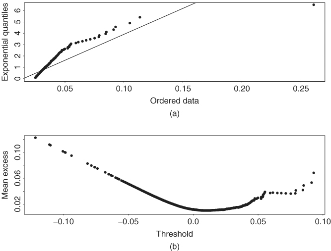
When ξ = 0, the GPD in Eq. (7.31) reduces to an exponential distribution. This result motivates the use of a QQ plot of excess returns over a threshold against exponential distribution to infer the tail behavior of the returns. If ξ = 0, then the QQ plot should be linear. Figure 7.6(a) shows the QQ plot of daily negative IBM log returns used in this chapter with threshold 0.025. The nonlinear feature of the plot clearly shows that the left tail of the daily IBM log returns is heavier than that of a normal distribution, that is, ξ ≠ 0.
Figure 7.6 Plots for daily negative IBM log returns from July 3, 1962, to December 31, 1998. (a) QQ plot of excess returns over threshold 2.5% and (b) mean excess plot.
7.7.1.1 R and S-Plus Commands Used to Produce Figure 7.6
> par(mfcol=c(2,1))
> qplot(-ibm,threshold=0.025,main='Negative daily IBM
log returns')
> meplot(-ibm)
> title(main='Mean excess plot')
7.7.2 Mean Excess Function
Given a high threshold ηo, suppose that the excess r − ηo follows a GPD with parameter ξ and ψ(ηo), where 0 < ξ < 1. Then the mean excess over the threshold ηo is
![]()
For any η > ηo, define the mean excess function e(η) as
![]()
In other words, for any y > 0,
![]()
Thus, for a fixed ξ, the mean excess function is a linear function of y = η − ηo. This result leads to a simple graphical method to infer the appropriate threshold value ηo for the GPD. Define the empirical mean excess function as
7.32 ![]()
where Nη is the number of returns that exceed η and ![]() are the values of the corresponding returns. See the next subsection for more information on the notation. The scatterplot of eT(η) against η is called the mean excess plot, which should be linear in η for η > ηo under the GPD. The plot is also called mean residual life plot. Figure 7.6(b) shows the mean excess plot of the daily negative IBM log returns. It shows that, among others, a threshold of about 3% is reasonable for the negative return series. In the evir package of R and S-Plus, the command for mean excess plot is meplot.
are the values of the corresponding returns. See the next subsection for more information on the notation. The scatterplot of eT(η) against η is called the mean excess plot, which should be linear in η for η > ηo under the GPD. The plot is also called mean residual life plot. Figure 7.6(b) shows the mean excess plot of the daily negative IBM log returns. It shows that, among others, a threshold of about 3% is reasonable for the negative return series. In the evir package of R and S-Plus, the command for mean excess plot is meplot.
7.7.3 New Approach to Modeling Extreme Values
Using the statistical result in Eq. (7.30) and considering jointly the exceedances and exceeding times, Smith (1989) proposes a two-dimensional Poisson process to model ![]() . This approach was used by Tsay (1999) to study VaR in risk management. We follow the same approach.
. This approach was used by Tsay (1999) to study VaR in risk management. We follow the same approach.
Assume that the baseline time interval is D, which is typically a year. In the United States, D = 252 is used as there are typically 252 trading days in a year. Let t be the time interval of the data points (e.g., daily) and denote the data span by t = 1, 2, … , T, where T is the total number of data points. For a given threshold η, the exceeding times over the threshold are denoted by {ti, i = 1, … , Nη} and the observed log return at ti is ![]() . Consequently, we focus on modeling
. Consequently, we focus on modeling ![]() for i = 1, … , Nη, where Nη depends on the threshold η.
for i = 1, … , Nη, where Nη depends on the threshold η.
The new approach to applying the extreme value theory is to postulate that the exceeding times and the associated returns [i.e., ![]() ] jointly form a two-dimensional Poisson process with intensity measure given by
] jointly form a two-dimensional Poisson process with intensity measure given by
where
![]()
0 ≤ D1 ≤ D2 ≤ T, r > η, α > 0, β, and ξ are parameters, and the notation [x]+ is defined as [x]+ = max(x, 0). This intensity measure says that the occurrence of exceeding the threshold is proportional to the length of the time interval [D1, D2] and the probability is governed by a survival function similar to the exponent of the CDF F*(r) in Eq. (7.16). A survival function of a random variable X is defined as S(x) = Pr(X > x) = 1 − Pr(X ≤ x) = 1 − CDF(x). When ξ = 0, the intensity measure is taken as the limit of ξ → 0; that is,
![]()
In Eq. (7.33), the length of time interval is measured with respect to the baseline interval D.
The idea of using the intensity measure in Eq. (7.33) becomes clear when one considers its implied conditional probability of r = x + η given r > η over the time interval [0, D], where x > 0,
![]()
which is precisely the survival function of the conditional distribution given in Eq. (7.30). This survival function is obtained from the extreme limiting distribution for maximum in Eq. (7.16). We use survival function here because it denotes the probability of exceedance.
The relationship between the limiting extreme value distribution in Eq. (7.16) and the intensity measure in Eq. (7.33) directly connects the new approach of extreme value theory to the traditional one.
Mathematically, the intensity measure in Eq. (7.33) can be written as an integral of an intensity function:
![]()
where the intensity function λ(t, z;ξ, α, β) is defined as
where
Using the results of a Poisson process, we can write down the likelihood function for the observed exceeding times and their corresponding returns ![]() over the two-dimensional space
over the two-dimensional space ![]() as
as
7.35 ![]()
The parameters ξ, α, and β can then be estimated by maximizing the logarithm of this likelihood function. Since the scale parameter α is nonnegative, we use ln(α) in the estimation.
Example 7.7
Consider again the daily log returns of IBM stock from July 3, 1962, to December 31, 1998. There are 9190 daily returns. Table 7.3 gives some estimation results of the parameters ξ, α, and β for three choices of the threshold when the negative series { − rt} is used. As mentioned before, we use the negative series { − rt}, instead of {rt} because we focus on holding a long financial position. The table also shows the number of exceeding times for a given threshold. It is seen that the chance of dropping 2.5% or more in a day for IBM stock occurred with probability 310/9190 ≈ 3.4%. Because the sample mean of IBM stock returns is not zero, we also consider the case when the sample mean is removed from the original daily log returns. From the table, removing the sample mean has little impact on the parameter estimates. These parameter estimates are used next to calculate VaR, keeping in mind that in a real application one needs to check carefully the adequacy of a fitted Poisson model. We discuss methods of model checking in the next section.
Table 7.3 Estimation Results of a Two-Dimensional Homogeneous Poisson Model for Daily Negative Log Returns of IBM Stock from July 3, 1962 to December 31, 1998a
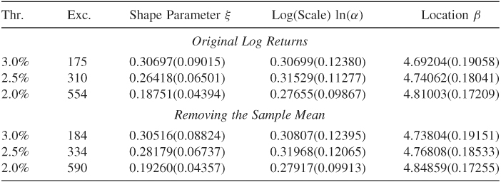
aThe baseline time interval is 252 (i.e., 1 year). The numbers in parentheses are standard errors, where Thr. and Exc. stand for threshold and the number of exceedings.
7.7.4 VaR Calculation Based on the New Approach
As shown in Eq. (7.30), the two-dimensional Poisson process model used, which employs the intensity measure in Eq. (7.33), has the same parameters as those of the extreme value distribution in Eq. (7.16). Therefore, one can use the same formula as that of Eq. (7.28) to calculate VaR of the new approach. More specifically, for a given upper tail probability p, the (1 − p)th quantile of the log return rt is
where D is the baseline time interval used in estimation. In the United States, one typically uses D = 252, which is approximately the number of trading days in a year.
Example 7.8
Consider again the case of holding a long position of IBM stock valued at $10 million. We use the estimation results of Table 7.3 to calculate 1-day horizon VaR for the tail probabilities of 0.05 and 0.01.
- Case I: Use the original daily log returns. The three choices of threshold η result in the following VaR values:
1. η = 3.0%: VaR(5%) = $228,239, VaR(1%) = $359.303.
2. η = 2.5%: VaR(5%) = $219,106, VaR(1%) = $361,119.
3. η = 2.0%: VaR(5%) = $212,981, VaR(1%) = $368.552.
- Case II: The sample mean of the daily log returns is removed. The three choices of threshold η result in the following VaR values:
1. η = 3.0%: VaR(5%) = $232,094, VaR(1%) = $363,697.
2. η = 2.5%: VaR(5%) = $225,782, VaR(1%) = $364,254.
3. η = 2.0%: VaR(5%) = $217,740, VaR(1%) = $372,372.
As expected, removing the sample mean, which is positive, slightly increases the VaR. However, the VaR is rather stable among the three threshold values used. In practice, we recommend that one removes the sample mean first before applying this new approach to VaR calculation.
Discussion
Compared with the VaR of Example 7.6 that uses the traditional extreme value theory, the new approach provides a more stable VaR calculation. The traditional approach is rather sensitive to the choice of the subperiod length n.
The command pot of the R package evir can be used to perform the estimation of the POT model. We demonstrate it below using the negative log returns of IBM stock. As expected, the results are very close to those obtained before.
7.7.4.1 R Demonstration Using POT Command
> library(evir)
> m3=pot(nibm,0.025)
> m3
$n
[1] 9190
$period
[1] 1 9190
$data
[1] 0.03288483 0.02648772 0.02817316 .....
$span
[1] 9189
$threshold
[1] 0.025
$p.less.thresh
[1] 0.9662677
$n.exceed
[1] 310
$par.ests
xi sigma mu beta
0.264078835 0.003182365 0.007557534 0.007788551
$par.ses
xi sigma mu
0.0229175739 0.0001808472 0.0007675515
$varcov
[,1] [,2] [,3]
[1,] 5.252152e-04 -2.873160e-06 -6.970497e-07
[2,] -2.873160e-06 3.270571e-08 -7.907532e-08
[3,] -6.970497e-07 -7.907532e-08 5.891353e-07
$intensity %intensity function of exceeding the threshold
[1] 0.03373599
> plot(m3) % model checking
Make a plot selection (or 0 to exit):
1: plot: Point Process of Exceedances
2: plot: Scatterplot of Gaps
3: plot: Qplot of Gaps
4: plot: ACF of Gaps
5: plot: Scatterplot of Residuals
6: plot: Qplot of Residuals
7: plot: ACF of Residuals
8: plot: Go to GPD Plots
Selection:
> riskmeasures(m3,c(0.95,0.99,0.999))
p quantile sfall
[1,] 0.950 0.02208860 0.03162728
[2,] 0.990 0.03616686 0.05075740
[3,] 0.999 0.07019419 0.09699513
7.7.5 Alternative Parameterization
As mentioned before, for a given threshold η, the GPD can also be parameterized by the shape parameter ξ and the scale parameter ψ(η) = α + ξ(η − β). This is the parameterization used in the evir package of R and S-Plus. Specifically, (xi,beta) of R and S-Plus corresponds to [ξ, ψ(η)] of this chapter. The command for estimating a GPD model in R and S-Plus is gpd. The output format for S-Plus is slightly different from that of R. For illustration, consider the daily negative IBM log return series from 1962 to 1998. The results of R are given below.
7.7.5.1 R Demonstration
Data are negative IBM log returns. The following output was edited:
> library(evir)
> mgpd=gpd(nibm,threshold=0.025)
> names(mgpd)
[1] "n" "data" "threshold" "p.less.thresh"
[5] "n.exceed" "method" "par.ests" "par.ses"
[9] "varcov" "information" "converged" "nllh.final"
> mgpd
$n
[1] 9190
$data
[1] 0.03288483 0.02648772 0.02817316 0.03618692 ....
$threshold
[1] 0.025
$p.less.thresh %Percentage of data below the threshold.
[1] 0.9662677
$n.exceed % Number of exceedances
[1] 310
$method
[1] "ml"
$par.ests
xi beta
0.264184649 0.007786063
$par.ses
xi beta
0.0662137508 0.0006427826
$varcov
[,1] [,2]
[1,] 4.384261e-03 -2.461142e-05
[2,] -2.461142e-05 4.131694e-07
> par(mfcol=c(2,2)) %Plots for residual analysis
> plot(mgpd)
Make a plot selection (or 0 to exit):
1: plot: Excess Distribution
2: plot: Tail of Underlying Distribution
3: plot: Scatterplot of Residuals
4: plot: QQplot of Residuals
Selection:
Note that the results are very close to those in Table 7.3, where percentage log returns are used. The estimates of ξ and ψ(η) are 0.26418 and α + ξ(η − β) = exp(0.31529) + (0.26418)(2.5 − 4.7406) = 0.77873, respectively, in Table 7.3. In terms of log returns, the estimate of ψ(η) is 0.007787, which is the same as the R and S-Plus estimate.
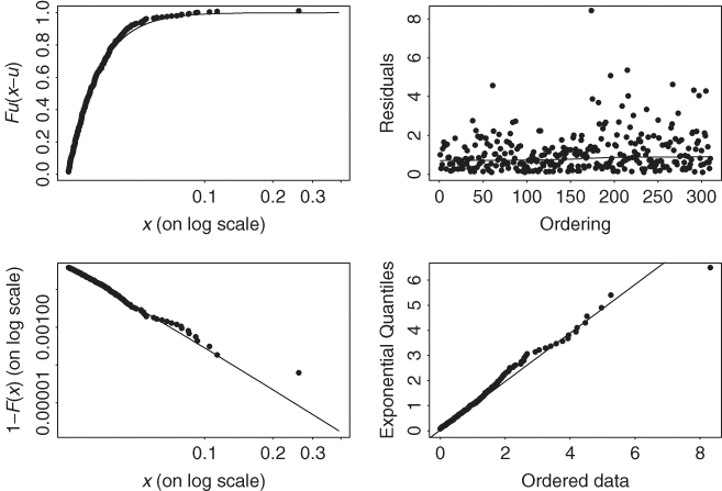
Figure 7.7 shows the diagnostic plots for the GPD fit to the daily negative log returns of IBM stock. The QQ plot (lower right panel) and the tail probability estimate (in log scale and in the lower left panel) show some minor deviation from a straight line, indicating further improvement is possible.
Figure 7.7 Diagnostic plots for GPD fit to daily negative log returns of IBM stock from July 3, 1962, to December 31, 1998.
From the conditional distributions in Eqs. (7.29) and (7.30) and the GPD in Eq. (7.31), we have
![]()
where y = x + η with x > 0. If we estimate the CDF F(η) of the returns by the empirical CDF, then
![]()
where Nη is the number of exceedances of the threshold η and T is the sample size. Consequently, by Eq. (7.31),
This leads to an alternative estimate of the quantile of F(y) for use in VaR calculation. Specifically, for a small upper tail probability p, let q = 1 − p. Then, by solving for y, we can estimate the qth quantile of F(y), denoted by VaRq, by
7.37 ![]()
where, as before, η is the threshold, T is the sample size, Nη is the number of exceedances, and ψ(η) and ξ are the scale and shape parameters of the GPD distribution. This method to VaR calculation is used in R and S-Plus.
As mentioned before in Section 7.2.4, expected shortfall (ES) associated with a given VaR is a useful risk measure. It is defined as the expected loss given that the VaR is exceeded. For generalized Pareto distribution, ES assumes a simple form. Specifically, for a given tail probability p, let q = 1 − p and denote the value at risk by VaRq. Then, the expected shortfall is defined by
7.38 ![]()
Using properties of the GPD, it can be shown that
![]()
provided that 0 < ξ < 1. Consequently, we have
![]()
To illustrate the new method to VaR and ES calculations, we again use the daily negative log returns of IBM stock with threshold 2.5%. In the evir package of R and S-Plus, the command to compute VaR and ES via the peak over threshold method is riskmeasures:
> riskmeasures(mgpd,c(0.95,0.99,0.999))
p quantile sfall
[1,] 0.950 0.02208959 0.03162619
[2,] 0.990 0.03616405 0.05075390
[3,] 0.999 0.07018944 0.09699565
From the output, the VaR values for the financial position of $10 million are $220, 889 and $361, 661, respectively, for tail probability of 0.05 and 0.01. These two values are rather close to those given in Example 7.8 that are based on the method of the previous section. The expected shortfalls for the financial position are $316, 272 and $507, 576, respectively, for tail probability of 0.05 and 0.01.
7.7.6 Use of Explanatory Variables
The two-dimensional Poisson process model discussed earlier is homogeneous because the three parameters ξ, α, and β are constant over time. In practice, such a model may not be adequate. Furthermore, some explanatory variables are often available that may influence the behavior of the log returns rt. A nice feature of the new extreme value theory approach to VaR calculation is that it can easily take explanatory variables into consideration. We discuss such a framework in this section. In addition, we also discuss methods that can be used to check the adequacy of a fitted two-dimensional Poisson process model.
Suppose that ![]() is a vector of v explanatory variables that are available prior to time t. For asset returns, the volatility
is a vector of v explanatory variables that are available prior to time t. For asset returns, the volatility ![]() of rt discussed in Chapter 3 is an example of explanatory variables. Another example of explanatory variables in the U.S. equity markets is an indicator variable denoting the meetings of the Federal Open Market Committee. A simple way to make use of explanatory variables is to postulate that the three parameters ξ, α, and β are time varying and are linear functions of the explanatory variables. Specifically, when explanatory variables
of rt discussed in Chapter 3 is an example of explanatory variables. Another example of explanatory variables in the U.S. equity markets is an indicator variable denoting the meetings of the Federal Open Market Committee. A simple way to make use of explanatory variables is to postulate that the three parameters ξ, α, and β are time varying and are linear functions of the explanatory variables. Specifically, when explanatory variables ![]() are available, we assume that
are available, we assume that
If ![]() , then the shape parameter ξt = γ0, which is time invariant. Thus, testing the significance of
, then the shape parameter ξt = γ0, which is time invariant. Thus, testing the significance of ![]() can provide information about the contribution of the explanatory variables to the shape parameter. Similar methods apply to the scale and location parameters. In Eq. (7.39), we use the same explanatory variables for all three parameters ξt, ln(αt), and βt. In an application, different explanatory variables may be used for different parameters.
can provide information about the contribution of the explanatory variables to the shape parameter. Similar methods apply to the scale and location parameters. In Eq. (7.39), we use the same explanatory variables for all three parameters ξt, ln(αt), and βt. In an application, different explanatory variables may be used for different parameters.
When the three parameters of the extreme value distribution are time varying, we have an inhomogeneous Poisson process. The intensity measure becomes
7.40 ![]()
The likelihood function of the exceeding times and returns ![]() becomes
becomes
![]()
which reduces to
if one assumes that the parameters ξt, αt, and βt are constant within each trading day, where g(z;ξt, αt, βt) and S(η;ξt, αt, βt) are given in Eqs. (7.34) and (7.33), respectively. For given observations {![]() }, the baseline time interval D, and the threshold η, the parameters in Eq. (7.39) can be estimated by maximizing the logarithm of the likelihood function in Eq. (7.41). Again we use ln(αt) to satisfy the positive constraint of αt.
}, the baseline time interval D, and the threshold η, the parameters in Eq. (7.39) can be estimated by maximizing the logarithm of the likelihood function in Eq. (7.41). Again we use ln(αt) to satisfy the positive constraint of αt.
Remark
The parameterization in Eq. (7.39) is similar to that of the volatility models of Chapter 3 in the sense that the three parameters are exact functions of the available information at time t. Other functions can be used if necessary. □
7.7.7 Model Checking
Checking an entertained two-dimensional Poisson process model for exceedance times and excesses involves examining three key features of the model. The first feature is to verify the adequacy of the exceedance rate, the second feature is to examine the distribution of exceedances, and the final feature is to check the independence assumption of the model. We discuss briefly some statistics that are useful for checking these three features. These statistics are based on some basic statistical theory concerning distributions and stochastic processes.
7.7.7.1 Exceedance Rate
A fundamental property of univariate Poisson processes is that the time durations between two consecutive events are independent and exponentially distributed. To exploit a similar property for checking a two-dimensional process model, Smith and Shively (1995) propose examining the time durations between consecutive exceedances. If the two-dimensional Poisson process model is appropriate for the exceedance times and excesses, the time duration between the ith and (i − 1)th exceedances should follow an exponential distribution. More specifically, letting t0 = 0, we expect that
![]()
are iid as a standard exponential distribution. Because daily returns are discrete-time observations, we employ the time durations
and use the QQ plot to check the validity of the iid standard exponential distribution. If the model is adequate, the QQ plot should show a straight line through the origin with unit slope.
7.7.7.2 Distribution of Excesses
Under the two-dimensional Poisson process model considered, the conditional distribution of the excess xt = rt − η over the threshold η is a GPD with shape parameter ξt and scale parameter ψt = αt + ξt(η − βt). Therefore, we can make use of the relationship between a standard exponential distribution and GPD, and define
If the model is adequate, ![]() are independent and exponentially distributed with mean 1; see also Smith (1999). We can then apply the QQ plot to check the validity of the GPD assumption for excesses.
are independent and exponentially distributed with mean 1; see also Smith (1999). We can then apply the QQ plot to check the validity of the GPD assumption for excesses.
7.7.7.3 Independence
A simple way to check the independence assumption, after adjusting for the effects of explanatory variables, is to examine the sample autocorrelation functions of ![]() and
and ![]() . Under the independence assumption, we expect that both
. Under the independence assumption, we expect that both ![]() and
and ![]() have no serial correlations.
have no serial correlations.
7.7.8 An Illustration
In this section, we apply a two-dimensional inhomogeneous Poisson process model to the daily log returns, in percentages, of IBM stock from July 3, 1962, to December 31, 1998. We focus on holding a long position of $10 million. The analysis enables us to compare the results with those obtained before by using other approaches to calculating VaR.
We begin by pointing out that the two-dimensional homogeneous model of Example 7.7 needs further refinements because the fitted model fails to pass the model checking statistics of the previous section. Figures 7.8(a) and 7.8(b) show the autocorrelation functions of the statistics ![]() and
and ![]() , defined in Eqs. (7.42) and (7.43), of the homogeneous model when the threshold is η = 2.5%. The horizontal lines in the plots denote asymptotic limits of two standard errors. It is seen that both
, defined in Eqs. (7.42) and (7.43), of the homogeneous model when the threshold is η = 2.5%. The horizontal lines in the plots denote asymptotic limits of two standard errors. It is seen that both ![]() and
and ![]() series have some significant serial correlations. Figures 7.9(a) and 7.9(b) show the QQ plots of the
series have some significant serial correlations. Figures 7.9(a) and 7.9(b) show the QQ plots of the ![]() and
and ![]() series. The straight line in each plot is the theoretical line, which passes through the origin and has a unit slope under the assumption of a standard exponential distribution. The QQ plot of
series. The straight line in each plot is the theoretical line, which passes through the origin and has a unit slope under the assumption of a standard exponential distribution. The QQ plot of ![]() shows some discrepancy.
shows some discrepancy.
Figure 7.8 Sample autocorrelation functions of the z and w measures for two-dimensional Poisson models. Parts (a) and (b) are for homogeneous model and parts (c) and (d) are for inhomogeneous model. Data are daily mean-corrected log returns, in percentages, of IBM stock from July 3, 1962, to December 31, 1998, and the threshold is 2.5%. A long financial position is used.
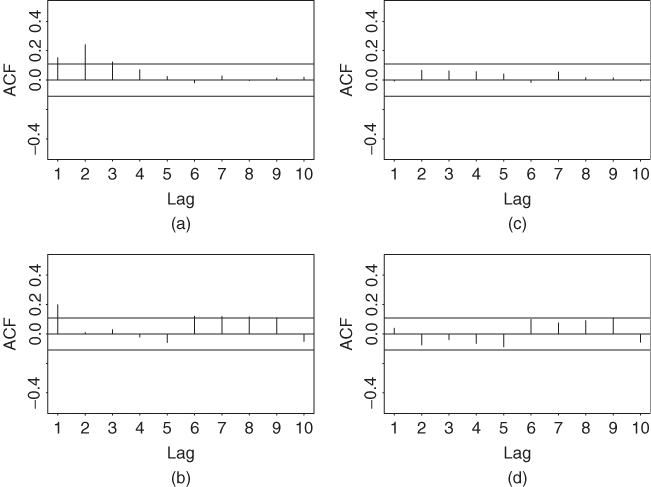
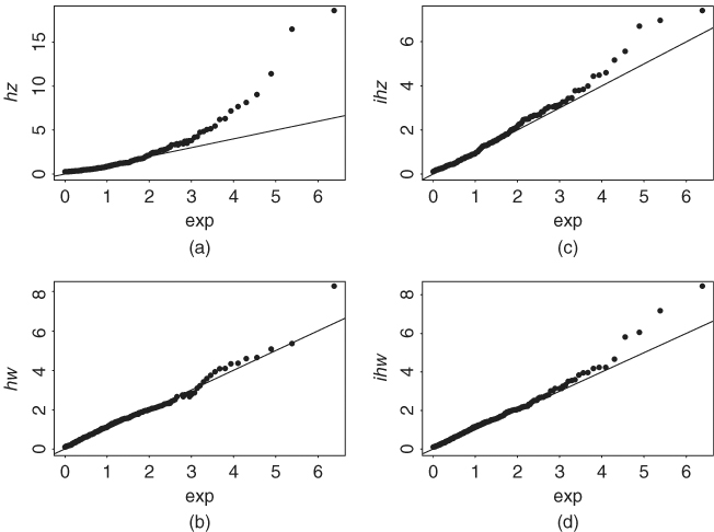
Figure 7.9 Quantile-to-quantile plot of z and w measures for two-dimensional Poisson models. Parts (a) and (b) are for homogeneous model and parts (c) and (d) are for inhomogeneous model. Data are daily mean-corrected log returns, in percentages, of IBM stock from July 3, 1962, to December 31, 1998, and the threshold is 2.5%. A long financial position is used.
To refine the model, we use the mean-corrected log return series
![]()
where rt is the daily log return in percentages, and employ the following explanatory variables:
1. x1t: an indicator variable for October, November, and December. That is, x1t = 1 if t is in October, November, or December. This variable is chosen to take care of the fourth-quarter effect (or year-end effect), if any, on the daily IBM stock returns.
2. x2t: an indicator variable for the behavior of the previous trading day. Specifically, x2t = 1 if and only if the log return ![]() . Since we focus on holding a long position with threshold 2.5%, an exceedance occurs when the daily price drops over 2.5%. Therefore, x2t is used to capture the possibility of panic selling when the price of IBM stock dropped 2.5% or more on the previous trading day.
. Since we focus on holding a long position with threshold 2.5%, an exceedance occurs when the daily price drops over 2.5%. Therefore, x2t is used to capture the possibility of panic selling when the price of IBM stock dropped 2.5% or more on the previous trading day.
3. x3t: a qualitative measurement of volatility, which is the number of days between t − 1 and t − 5 (inclusive) that has a log return with magnitude exceeding the threshold. In our case, x3t is the number of ![]() satisfying
satisfying ![]() 2.5% for i = 1, … , 5.
2.5% for i = 1, … , 5.
4. x4t: an annual trend defined as x4t = (year of time t − 1961)/38. This variable is used to detect any trend in the behavior of extreme returns of IBM stock.
5. x5t: a volatility series based on a Gaussian GARCH(1,1) model for the mean-corrected series ![]() . Specifically, x5t = σt, where
. Specifically, x5t = σt, where ![]() is the conditional variance of the GARCH(1,1) model
is the conditional variance of the GARCH(1,1) model
![]()
These five explanatory variables are all available at time t − 1. We use two volatility measures (x3t and x5t) to study the effect of market volatility on VaR. As shown in Example 7.3 by the fitted AR(2)–GARCH(1,1) model, the serial correlations in rt are weak so that we do not entertain any ARMA model for the mean equation.
Using the prior five explanatory variables and deleting insignificant parameters, we obtain the estimation results shown in Table 7.4. Figures 7.8(c) and 7.8(d) and Figures 7.9(c) and 7.9(d) show the model checking statistics for the fitted two-dimensional inhomogeneous Poisson process model when the threshold is η = 2.5%. All autocorrelation functions of ![]() and
and ![]() are within the asymptotic two standard error limits. The QQ plots also show marked improvements as they indicate no model inadequacy. Based on these checking results, the inhomogeneous model seems adequate.
are within the asymptotic two standard error limits. The QQ plots also show marked improvements as they indicate no model inadequacy. Based on these checking results, the inhomogeneous model seems adequate.
Table 7.4 Estimation Results of Two-Dimensional Inhomogeneous Poisson Process Model for Daily Log Returns, in Percentages, of IBM Stock from July 3, 1962 to December 31, 1998a
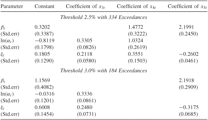
aFour explanatory variables defined in the text are used. The model is for holding a long position on IBM stock. The sample mean of the log returns is removed from the data.
Consider the case of threshold 2.5%. The estimation results show the following:
1. All three parameters of the intensity function depend significantly on the annual time trend. In particular, the shape parameter has a negative annual trend, indicating that the log returns of IBM stock are moving farther away from normality as time passes. Both the location and scale parameters increase over time.
2. Indicators for the fourth quarter, x1t, and for panic selling, x2t, are not significant for all three parameters.
3. The location and shape parameters are positively affected by the volatility of the GARCH(1,1) model; see the coefficients of x5t. This is understandable because the variability of log returns increases when the volatility is high. Consequently, the dependence of log returns on the tail index is reduced.
4. The scale and shape parameters depend significantly on the qualitative measure of volatility. Signs of the estimates are also plausible.
The explanatory variables for December 31, 1998, assumed the values x3, 9190 = 0, x4, 9190 = 0.9737, and x5, 9190 = 1.9766. Using these values and the fitted model in Table 7.4, we obtain
![]()
Assume that the tail probability is 0.05. The VaR quantile shown in Eq. (7.36) gives VaR = 3.03756%. Consequently, for a long position of $10 million, we have
![]()
If the tail probability is 0.01, the VaR is $497, 425. The 5% VaR is slightly larger than that of Example 7.3, which uses a Gaussian AR(2)–GARCH(1,1) model. The 1% VaR is larger than that of Case 1 of Example 7.3. Again, as expected, the effect of extreme values (i.e., heavy tails) on VaR is more pronounced when the tail probability used is small.
An advantage of using explanatory variables is that the parameters are adaptive to the change in market conditions. For example, the explanatory variables for December 30, 1998, assumed the values x3, 9189 = 1, x4, 9189 = 0.9737, and x5, 9189 = 1.8757. In this case, we have
![]()
The 95% quantile (i.e., the tail probability is 5%) then becomes 2.69139%. Consequently, the VaR is
![]()
If the tail probability is 0.01, then VaR becomes $448, 323. Based on this example, the homogeneous Poisson model shown in Example 7.8 seems to underestimate the VaR.