

Chapter Two
RATE OF CHANGE: THE DERIVATIVE
Contents
2.1 Instantaneous Rate of Change
Defining Instantaneous Velocity Using the Idea of a Limit
Visualizing the Derivative: Slope of the Graph and Slope of the Tangent Line
Estimating the Derivative of a Function Given Numerically
Finding the Derivative of a Function Given Graphically
What Does the Derivative Tell Us Graphically?
Estimating the Derivative of a Function Given Numerically
Finding the Derivative of a Function Given by a Formula
2.3 Interpretations of the Derivative
An Alternative Notation for the Derivative
Using Units to Interpret the Derivative
Using the Derivative to Estimate Values of a Function
What Does the Second Derivative Tell Us?
Interpretation of the Second Derivative as a Rate of Change
Graphs of Cost and Revenue Functions
Limits, Continuity, and the Definition of the Derivative
2.1 INSTANTANEOUS RATE OF CHANGE
Chapter 1 introduced the average rate of change of a function over an interval. In this section, we consider the rate of change of a function at a point. We saw in Chapter 1 that when an object is moving along a straight line, the average rate of change of position with respect to time is the average velocity. If position is expressed as y = f(t), where t is time, then
![]()
If you drive 200 miles in 4 hours, your average velocity is 200/4 = 50 miles per hour. Of course, this does not mean that you travel at exactly 50 mph the entire trip. Your velocity at a given instant during the trip is shown on your speedometer, and this is the quantity that we investigate now.
Instantaneous Velocity
We throw a grapefruit straight upward into the air. Table 2.1 gives its height, y, at time t. What is the velocity of the grapefruit at exactly t = 1? We use average velocities to estimate this quantity.
The average velocity on the interval 0 ≤ t ≤ 1 is 84 ft/sec and the average velocity on the interval 1 ≤ t ≤ 2 is 52 ft/sec. Notice that the average velocity before t = 1 is larger than the average velocity after t = 1 since the grapefruit is slowing down. We expect the velocity at t = 1 to be between these two average velocities. How can we find the velocity at exactly t = 1? We look at what happens near t = 1 in more detail. Suppose that we find the average velocities on either side of t = 1 over smaller and smaller intervals, as in Figure 2.1. Then, for example,
![]()
We expect the instantaneous velocity at t = 1 to be between the average velocities on either side of t = 1. In Figure 2.1, the values of the average velocity before t = 1 and the average velocity after t = 1 get closer together as the size of the interval shrinks. For the smallest intervals in Figure 2.1, both velocities are 68.0 ft/sec (to one decimal place), so we say the velocity at t = 1 is 68.0 ft/sec (to one decimal place).

Figure 2.1: Average velocities over intervals on either side of t = 1 showing successively smaller intervals
Of course, if we showed more decimal places, the average velocities before and after t = 1 would no longer agree. To calculate the velocity at t = 1 to more decimal places of accuracy, we take smaller and smaller intervals on either side of t = 1 until the average velocities agree to the number of decimal places we want. In this way, we can estimate the velocity at t = 1 to any accuracy.
Defining Instantaneous Velocity Using the Idea of a Limit
When we take smaller intervals near t = 1, it turns out that the average velocities for the grapefruit are always just above or just below 68 ft/sec. It seems natural, then, to define velocity at the instant t = 1 to be 68 ft/sec. This is called the instantaneous velocity at this point. Its definition depends on our being convinced that smaller and smaller intervals provide average velocities that come arbitrarily close to 68. This process is referred to as taking the limit.
The instantaneous velocity of an object at time t is defined to be the limit of the average velocity of the object over shorter and shorter time intervals containing t.
Notice that the instantaneous velocity seems to be exactly 68, but what if it were 68.000001? How can we be sure that we have taken small enough intervals? Showing that the limit is exactly 68 requires more precise knowledge of how the velocities were calculated and of the limiting process; see the Focus on Theory section.
Instantaneous Rate of Change
We can define the instantaneous rate of change of any function y = f(t) at a point t = a. We mimic what we did for velocity and look at the average rate of change over smaller and smaller intervals.
The instantaneous rate of change of f at a, also called the rate of change of f at a, is defined to be the limit of the average rates of change of f over shorter and shorter intervals around a.
Since the average rate of change is a difference quotient of the form Δy/Δt, the instantaneous rate of change is a limit of difference quotients. In practice, we often approximate a rate of change by one of these difference quotients.
| Example 1 | The quantity (in mg) of a drug in the blood at time t (in minutes) is given by Q = 25(0.8)t. Estimate the rate of change of the quantity at t = 3 and interpret your answer. |
| Solution | We estimate the rate of change at t = 3 by computing the average rate of change over intervals near t = 3. We can make our estimate as accurate as we like by choosing our intervals small enough. Let's look at the average rate of change over the interval 3 ≤ t ≤ 3.01:
A reasonable estimate for the rate of change of the quantity at t = 3 is −2.85. Since Q is in mg and t in minutes, the units of ΔQ/Δt are mg/minute. Since the rate of change is negative, the quantity of the drug is decreasing. After 3 minutes, the quantity of the drug in the body is decreasing at 2.85 mg/minute. |
In Example 1, we estimated the rate of change using an interval to the right of the point (t = 3 to t = 3.01). In the next section we briefly consider other ways of making estimates.
The Derivative at a Point
The instantaneous rate of change of a function f at a point a is so important that it is given its own name, the derivative of f at a, denoted f′(a) (read “f-prime of a”). If we want to emphasize that f′(a) is the rate of change of f(x) as the variable x increases, we call f′(a) the derivative of f with respect to x at x = a. Notice that the derivative is just a new name for the rate of change of a function.
The derivative of f at a, written f′(a), is defined to be the instantaneous rate of change of f at the point a.
A definition of the derivative using a formula is given in the Focus on Theory section.
| Example 2 | Estimate f′(2) if f(x) = x3. |
| Solution | Since f′(2) is the derivative, or rate of change, of f(x) = x3 at 2, we look at the average rate of change over intervals near 2. Using the interval 2 ≤ x ≤ 2.001, we see that
The rate of change of f(x) at x = 2 appears to be approximately 12, so we estimate f′(2) = 12. |

Visualizing the Derivative: Slope of the Graph and Slope of the Tangent Line
Figure 2.2 shows the average rate of change of a function represented by the slope of the secant line joining points A and B. The derivative is found by taking the average rate of change over smaller and smaller intervals. In Figure 2.3, as point B moves toward point A, the secant line approaches the tangent line at point A. Thus, the derivative is represented by the slope of the tangent line to the graph at the point.

Figure 2.2: Visualizing the average rate of change of f between a and b

Figure 2.3: Visualizing the instantaneous rate of change of f at a
Alternatively, take the graph of a function around a point and “zoom in” to get a close-up view. (See Figure 2.4.) The more we zoom in, the more the graph appears to be straight. We call the slope of this line the slope of the graph at the point; it also represents the derivative.
The derivative of a function at the point A is equal to
- The slope of the graph of the function at A.
- The slope of the line tangent to the curve at A.

Figure 2.4: Finding the slope of a curve at a point by “zooming in”
The slope interpretation is often useful in gaining rough information about the derivative, as the following examples show.
| Example 3 | Use a graph of f(x) = x2 to determine whether each of the following quantities is positive, negative, or zero: (a) f′(1) (b) f′(−1) (c) f′(2) (d) f′(0) |
| Solution | Figure 2.5 shows tangent line segments to the graph of f(x) = x2 at the points x = 1, x = −1, x = 2, and x = 0. Since the derivative is the slope of the tangent line at the point, we have:
(a) f′(1) is positive. (b) f′(−1) is negative. (c) f′(2) is positive (and larger than f′(1)). (d) f′(0) = 0 since the graph has a horizontal tangent at x = 0. |

Figure 2.5: Tangent lines showing sign of derivative of f(x) = x2
| Example 4 | Estimate the derivative of f(x) = 2x at x = 0 graphically and numerically. |
| Solution | Graphically: If we draw a tangent line at x = 0 to the exponential curve in Figure 2.6, we see that it has a positive slope between 0.5 and 1. |

Figure 2.6: Graph of f(x) = 2x showing the derivative at x = 0
Numerically: To estimate the derivative at x = 0, we compute the average rate of change on an interval around 0.

Since using smaller intervals gives approximately the same values, it appears that the derivative is approximately 0.69317; that is, f′(0) ≈ 0.693.
| Example 5 | The graph of a function y = f(x) is shown in Figure 2.7. Indicate whether each of the following quantities is positive or negative, and illustrate your answers graphically.
(a) f′(1) (b) (c) f(4) − f(2)
|
| Solution | (a) Since f′(1) is the slope of the graph at x = 1, we see in Figure 2.8 that f′(1) is positive.
(b) The difference quotient (f(3) − f(1))/(3 − 1) is the slope of the secant line between x = 1 and x = 3. We see from Figure 2.9 that this slope is positive. (c) Since f(4) is the value of the function at x = 4 and f(2) is the value of the function at x = 2, the expression f(4) − f(2) is the change in the function between x = 2 and x = 4. Since f(4) lies below f(2), this change is negative. See Figure 2.10. |


Estimating the Derivative of a Function Given Numerically
If we are given a table of values for a function, we can estimate values of its derivative. To do this, we have to assume that the points in the table are close enough together that the function does not change wildly between them.
| Example 6 | The total acreage of farms in the US1 has decreased since 1980. See Table 2.2.
(a) What was the average rate of change in farm land between 1980 and 2000? (b) Estimate f′(1995) and interpret your answer in terms of farm land. |
| Solution | (a) Between 1980 and 2000,
Between 1980 and 2000, the amount of farm land was decreasing at an average rate of 4.7 million acres per year. (b) We use the interval from 1995 to 2000 to estimate the instantaneous rate of change at 1995:
In 1995, the amount of farm land was decreasing at a rate of approximately 3.6 million acres per year. |
Problems for Section 2.1
1. Figure 2.11 shows N = f(t), the number of farms in the US2 between 1930 and 2000 as a function of year, t.
(a) Is f′(1950) positive or negative? What does this tell you about the number of farms?
(b) Which is more negative: f′(1960) or f′(1980)? Explain.

2. Use the graph in Figure 2.7 to decide if each of the following quantities is positive, negative or approximately zero. Illustrate your answers graphically.
(a) The average rate of change of f(x) between x = 3 and x = 7.
(b) The instantaneous rate of change of f(x) at x = 3.
3. The position s of a car at time t is given in the following table.

(a) Find the average velocity over the interval 0 ≤ t ≤ 0.2.
(b) Find the average velocity over the interval 0.2 ≤ t ≤ 0.4.
(c) Use the previous answers to estimate the instantaneous velocity of the car at t = 0.2.
4. In a time of t seconds, a particle moves a distance of s meters from its starting point, where s = 4t2 + 3.
(a) Find the average velocity between t = 1 and t = 1 + h if:
(i) h = 0.1,
(ii) h = 0.01,
(iii) h = 0.001.
(b) Use your answers to part (a) to estimate the instantaneous velocity of the particle at time t = 1.
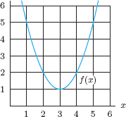
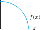
5. Figure 2.12 shows the cost, y = f(x), of manufacturing x kilograms of a chemical.
(a) Is the average rate of change of the cost greater between x = 0 and x = 3, or between x = 3 and x = 5? Explain your answer graphically.
(b) Is the instantaneous rate of change of the cost of producing x kilograms greater at x = 1 or at x = 4? Explain your answer graphically.
(c) What are the units of these rates of change?

6. The distance (in feet) of an object from a point is given by s(t) = t2, where time t is in seconds.
(a) What is the average velocity of the object between t = 2 and t = 5?
(b) By using smaller and smaller intervals around 2, estimate the instantaneous velocity at time t = 2.
7. (a) Using Table 2.3, find the average rate of change in the world's population, P, between 1975 and 2010.3 Give units.
(b) If P = f(t) with t in years, estimate f′ (2010) and give units.
Table 2.3 World population, in billions of people
![]()
8. The size, S, of a tumor (in cubic millimeters) is given by S = 2t, where t is the number of months since the tumor was discovered. Give units with your answers.
(a) What is the total change in the size of the tumor during the first six months?
(b) What is the average rate of change in the size of the tumor during the first six months?
(c) Estimate the rate at which the tumor is growing at t = 6. (Use smaller and smaller intervals.)
9. Let g(x) = 4x. Use small intervals to estimate g′(1).
10. (a) Let g(t) = (0.8)t. Use a graph to determine whether g′(2) is positive, negative, or zero.
(b) Use a small interval to estimate g′(2).
11. For the function shown in Figure 2.13, at what labeled points is the slope of the graph positive? Negative? At which labeled point does the graph have the greatest (i.e., most positive) slope? The least slope (i.e., negative and with the largest magnitude)?

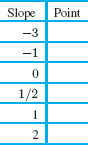
12. Match the points labeled on the curve in Figure 2.14 with the given slopes.

13. For the function f(x) = 3x, estimate f′(1). From the graph of f(x), would you expect your estimate to be greater than or less than the true value of f′(1)?
14. Table 2.4 gives P = f(t), the number of households, in millions, in the US with cable television t years since 1998.4
(a) Does f′(4) appear to be positive or negative? What does this tell you about the percent of households with cable television?
(b) Estimate f′(2). Estimate f′(10). Explain what each is telling you, in terms of cable television.
![]()
15. The following table gives the percent of the US population living in urban areas as a function of year.5

(a) Find the average rate of change of the percent of the population living in urban areas between 1890 and 1990.
(b) Estimate the rate at which this percent is increasing at the year 1990.
(c) Estimate the rate of change of this function for the year 1830 and explain what it is telling you.
16. (a) Graph f(x) = x2 and g(x) = x2 + 3 on the same axes. What can you say about the slopes of the tangent lines to the two graphs at the point x = 0? x = 1? x = 2? x = a, where a is any value?
(b) Explain why adding a constant to any function will not change the value of the derivative at any point.
17. The function in Figure 2.15 has f(4) = 25 and f′(4) = 1.5. Find the coordinates of the points A, B, C.

18. Use Figure 2.16 to fill in the blanks in the following statements about the function f at point A.
(a) f(__) = __
(b) f′(__) = __

19. Show how to represent the following on Figure 2.17.
(a) f(4)
(b) f(4) − f(2)
(c) ![]()
(d) f′(3)

20. For each of the following pairs of numbers, use Figure 2.17 to decide which is larger. Explain your answer.
(a) f(3) or f(4)?
(b) f(3) − f(2) or f(2) − f(1)?
(c) ![]()
(d) f′(1) or f′(4)?
21. Estimate the instantaneous rate of change of the function f(x) = x ln x at x = 1 and at x = 2. What do these values suggest about the concavity of the graph between 1 and 2?
22. On October 17, 2006, in an article called “US Population Reaches 300 Million,” the BBC reported that the US gains 1 person every 11 seconds. If f(t) is the US population in millions t years after October 17, 2006, find f(0) and f′(0).
23. The following table shows the number of hours worked in a week, f(t), hourly earnings, g(t), in dollars, and weekly earnings, h(t), in dollars, of production workers as functions of t, the year.6
(a) Indicate whether each of the following derivatives is positive, negative, or zero: f′(t), g′(t), h′(t). Interpret each answer in terms of hours or earnings.
(b) Estimate each of the following derivatives, and interpret your answers:
(i) f′(1970) and f′(1995)
(ii) g′(1970) and g′(1995)
(iii) h′(1970) and h′(1995)

2.2 THE DERIVATIVE FUNCTION
In Section 2.1 we looked at the derivative of a function at a point. In general, the derivative takes on different values at different points and is itself a function. Recall that the derivative is the slope of the tangent line to the graph at the point.
Finding the Derivative of a Function Given Graphically
| Example 1 | Estimate the derivative of the function f(x) graphed in Figure 2.18 at x = −2, −1, 0, 1, 2, 3, 4, 5.
Figure 2.18: Estimating the derivative graphically as the slope of a tangent line |
| Solution | From the graph, we estimate the derivative at any point by placing a straightedge so that it forms the tangent line at that point, and then using the grid to estimate the slope of the tangent line. For example, the tangent at x = −1 is drawn in Figure 2.18, and has a slope of about 2, so f′(−1) ≈ 2. Notice that the slope at x = −2 is positive and fairly large; the slope at x = −1 is positive but smaller. At x = 0, the slope is negative, by x = 1 it has become more negative, and so on. Some estimates of the derivative, to the nearest integer, are listed in Table 2.5. You should check these values yourself. Is the derivative positive where you expect? Negative? |

Table 2.5 Estimated values of derivative of function in Figure 2.18
![]()
The important point to notice is that for every x-value, there is a corresponding value of the derivative. The derivative, therefore, is a function of x.
For a function f, we define the derivative function, f′, by
![]()
| Example 2 | Plot the values of the derivative function calculated in Example 1. Compare the graphs of f′ and f. |
| Solution | Graphs of f and f′ are in Figures 2.19 and 2.20, respectively. Notice that f′ is positive (its graph is above the x-axis) where f is increasing, and f′ is negative (its graph is below the x-axis) where f is decreasing. The value of f′(x) is 0 where f has a maximum or minimum value (at approximately x = −0.4 and x = 3.7). |
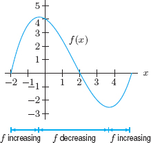
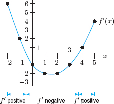
Figure 2.20: Estimates of the derivative, f′
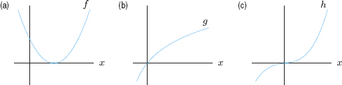
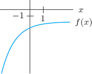
| Example 3 | The graph of f is in Figure 2.21. Which of the graphs (a)–(c) is a graph of the derivative, f′?
|
| Solution | Since the tangent of f(x) is horizontal at x = −1 and x = 2, the derivative is zero there. Therefore, the graph of f′(x) has x-intercepts at x = −1 and x = 2.
The function f is decreasing for x < −1, increasing for −1 < x < 2, and decreasing for x > 2. The derivative is positive (its graph is above the x-axis) where f is increasing, and the derivative is negative (its graph is below the x-axis) where f is decreasing. The correct graph is (c). |


What Does the Derivative Tell Us Graphically?
Where the derivative, f′, of a function is positive, the tangent to the graph of f is sloping up; where f′ is negative, the tangent is sloping down. If f′ = 0 everywhere, then the tangent is horizontal everywhere and so f is constant. The sign of the derivative f′ tells us whether the function f is increasing or decreasing.

The magnitude of the derivative gives us the magnitude of the rate of change of f. If f′ is large in magnitude, then the graph of f is steep (up if f′ is positive or down if f′ is negative); if f′ is small in magnitude, the graph of f is gently sloping.
Estimating the Derivative of a Function Given Numerically
If we are given a table of function values instead of a graph of the function, we can estimate values of the derivative.
| Example 4 | Table 2.6 gives values of c(t), the concentration (mg/cc) of a drug in the bloodstream at time t (min). Construct a table of estimated values for c′(t), the rate of change of c(t) with respect to t.
Table 2.6 Concentration of a drug as a function of time
|
| Solution | To estimate the derivative of c using the values in the table, we assume that the data points are close enough together that the concentration does not change wildly between them. From the table, we see that the concentration is increasing between t = 0 and t = 0.4, so we expect a positive derivative there. From t = 0.5 to t = 1.0, the concentration starts to decrease, and the rate of decrease gets larger and larger, so we would expect the derivative to be negative and of greater and greater magnitude.
We estimate the derivative for each value of t using a difference quotient. For example,
Similarly, we get the estimates
and so on. These values are tabulated in Table 2.7. Notice that the derivative has small positive values up until t = 0.4, and then it gets more and more negative, as we expected. |

Table 2.7 Derivative of concentration
![]()
Improving Numerical Estimates for the Derivative
In the previous example, our estimate for the derivative of c(t) at t = 0.2 used the point to the right. We found the average rate of change between t = 0.2 and t = 0.3. However, we could equally well have gone to the left and used the rate of change between t = 0.1 and t = 0.2 to approximate the derivative at 0.2. For a more accurate result, we could average these slopes, getting the approximation

Each of these methods of approximating the derivative gives a reasonable answer. We will usually estimate the derivative by going to the right.
Finding the Derivative of a Function Given by a Formula
If we are given a formula for a function f, can we come up with a formula for f′? Using the definition of the derivative, we often can. Indeed, much of the power of calculus depends on our ability to find formulas for the derivatives of all the familiar functions. This is explained in detail in Chapter 3. In the next example, we see how to guess a formula for the derivative.
| Example 5 | Guess a formula for the derivative of f(x) = x2. |
| Solution | We use difference quotients to estimate the values of f′(1), f′(2), and f′(3). Then we look for a pattern in these values which we use to guess a formula for f′(x).
Near x = 1, we have
Knowing the value of f′ at specific points cannot tell us the formula for f′, but it can be suggestive: knowing f′(1) ≈ 2, f′(2) ≈ 4, f′(3) ≈ 6 suggests that f′(x) = 2x. In Chapter 3, we show that this is indeed the case. |

Problems for Section 2.2
For Problems 1–6, graph the derivative of the given functions.
1.

2.

3.

4.

5.

6.

7. The graph of f(x) is given in Figure 2.22. Draw tangent lines to the graph at x = −2, x = −1, x = 0, and x = 2. Estimate f′(−2), f′(−1), f′(0), and f′(2).

8. The graph of f(x) is given in Figure 2.23. Estimate f′(1), f′(2), f′(3), f′(4), and f′(5).
9. In the graph of f in Figure 2.24, at which of the labeled x-values is
(a) f(x) greatest?
(b) f(x) least?
(c) f′(x) greatest?
(d) f′(x) least?

10. Find approximate values for f′(x) at each of the x-values given in the following table.
![]()
11. Using slopes to left and right of 0, estimate R′(0) if R(x) = 100(1.1)x.
For Problems 12–17, sketch the graph of f′(x).
12.

13.

14.

15.

16.
17.

Match the functions in Problems 18–21 with one of the derivatives in Figure 2.25.

18.

19.

20.

21.

22. A city grew in population throughout the 1980s and into the early 1990s. The population was at its largest in 1995, and then shrank until 2010. Let P = f(t) represent the population of the city t years since 1980. Sketch graphs of f(t) and f′(t), labeling the units on the axes.
23. Values of x and g(x) are given in the table. For what value of x does g′(x) appear to be closest to 3?

24. Draw a possible graph of y = f(x) given the following information about its derivative.
- f′(x) > 0 for x < −1
- f′(x) < 0 for x > −1
- f′(x) = 0 at x = −1
25. Draw apossible graph of a continuous function y = f(x) that satisfies the following three conditions:
- f′(x) > 0 for 1 < x < 3
- f′(x) < 0 for x < 1 and x > 3
- f′(x) = 0 at x = 1 and x = 3
26. A vehicle moving along a straight road has distance f(t) from its starting point at time t. Which of the graphs in Figure 2.26 could be f′(t) for the following scenarios? (Assume the scales on the vertical axes are all the same.)
(a) A bus on a popular route, with no traffic
(b) A car with no traffic and all green lights
(c) A car in heavy traffic conditions

27. (a) Let f(x) = ln x. Use small intervals to estimate f′(1), f′(2), f′(3), f′(4), and f′(5).
(b) Use your answers to part (a) to guess a formula for the derivative of f(x) = ln x.
28. Suppose f(x) = ![]() x3. Estimate f′(2), f′(3), and f′(4). What do you notice? Can you guess a formula for f′(x)?
x3. Estimate f′(2), f′(3), and f′(4). What do you notice? Can you guess a formula for f′(x)?
29. Match each property (a)–(d) with one or more of graphs (I)–(IV) of functions.
(a) f′(x) = 1 for all 0 ≤ x ≤ 4.
(b) f′(x) > 0 for all 0 ≤ x ≤ 4
(c) f′(2) = 1
(d) f′(1) = 2
(I)

(II)

(III)

(IV)

30. A child inflates a balloon, admires it for a while and then lets the air out at a constant rate. If V(t) gives the volume of the balloon at time t, then Figure 2.27 shows V′(t) as a function of t. At what time does the child:
(a) Begin to inflate the balloon?
(b) Finish inflating the balloon?
(c) Begin to let the air out?
(d) What would the graph of V′(t) look like if the child had alternated between pinching and releasing the open end of the balloon, instead of letting the air out at a constant rate?

2.3 INTERPRETATIONS OF THE DERIVATIVE
We have seen the derivative interpreted as a slope and as a rate of change. In this section, we see other interpretations. The purpose of these examples is not to make a catalog of interpretations but to illustrate the process of obtaining them. There is another notation for the derivative that is often helpful.
An Alternative Notation for the Derivative
So far we have used the notation f′ to stand for the derivative of the function f. An alternative notation for derivatives was introduced by the German mathematician Gottfried Wilhelm Leibniz (1646–1716) when calculus was first being developed. We know that f′(x) is approximated by the average rate of change over a small interval. If y = f(x), then the average rate of change is given by Δy/Δx. For small Δx, we have
![]()
Leibniz's notation for the derivative, dy/dx, is meant to remind us of this. If y = f(x), then we write
![]()
Leibniz's notation is quite suggestive, especially if we think of the letter d in dy/dx as standing for “small difference in . . . .” The notation dy/dx reminds us that the derivative is a limit of ratios of the form
![]()
The notation dy/dx is useful for determining the units for the derivative: the units for dy/dx are the units for y divided by (or “per”) the units for x.
The separate entities dy and dx officially have no independent meaning: they are part of one notation. In fact, a good formal way to view the notation dy/dx is to think of d/dx as a single symbol meaning “the derivative with respect to x of. . .”. Thus, dy/dx could be viewed as
![]()
On the other hand, many scientists and mathematicians really do think of dy and dx as separate entities representing “infinitesimally” small differences in y and x, even though it is difficult to say exactly how small “infinitesimal” is. It may not be formally correct, but it is very helpful intuitively to think of dy/dx as a very small change in y divided by a very small change in x.
For example, recall that if s = f(t) is the position of a moving object at time t, then v = f′(t) is the velocity of the object at time t. Writing
![]()
reminds us that v is a velocity since the notation suggests a distance, ds, over a time, dt, and we know that distance over time is velocity. Similarly, we recognize
![]()
as the slope of the graph of y = f(x) by remembering that slope is vertical rise, dy, over horizontal run, dx.
The disadvantage of the Leibniz notation is that it is awkward to specify the value at which a derivative is evaluated. To specify f′(2), for example, we have to write

Using Units to Interpret the Derivative
Suppose a body moves along a straight line. If s = f(t) gives the position in meters of the body from a fixed point on the line as a function of time, t, in seconds, then knowing that
![]()
tells us that when t = 2 sec, the body is moving at a velocity of 10 meters/sec. If the body continues to move at this velocity for a whole second (from t = 2 to t = 3), it would move an additional 10 meters.
In other words, if Δs represents the change in position during a time interval Δt, and if the body continues to move at this velocity, we have Δs = 10Δt, so
![]()
If the velocity is varying, this relationship is no longer exact. For small values of Δt, we have the Tangent Line Approximation
![]()
(See also page 107.) Notice that, for a given positive Δt, a large derivative gives large change in s; a small derivative gives small change in s. In general:
- The units of the derivative of a function are the units of the dependent variable divided by the units of the independent variable. In other words, the units of dA/dB are the units of A divided by the units of B.
- If the derivative of a function is not changing rapidly near a point, then the derivative is approximately equal to the change in the function when the independent variable increases by 1 unit.
The following examples illustrate how useful units can be in suggesting interpretations of the derivative.
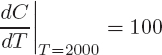
| Example 2 | The cost of extracting T tons of ore from a copper mine is C = f(T) dollars. What does it mean to say that f′(2000) = 100? |
| Solution | In the Leibniz notation,
Since C is measured in dollars and T is measured in tons, dC/dT is measured in dollars per ton. You can think of dC as the extra cost of extracting an extra dT tons of ore. So the statement
says that when 2000 tons of ore have already been extracted from the mine, the cost of extracting the next ton is approximately $100. Another way of saying this is that it costs about $100 to extract the 2001st ton. |

| Example 3 | If q = f(p) gives the number of thousands of tons of zinc produced when the price is p dollars per ton, then what are the units and the meaning of
|
| Solution | The units of dq/dp are the units of q over the units of p, or thousands of tons per dollar. You can think of dq as the extra zinc produced when the price increases by dp. The statement
tells us that the instantaneous rate of change of q with respect to p is 0.2 when p = 900. This means that when the price is $900, the quantity produced increases by about 0.2 thousand tons, or 200 tons more for a one-dollar increase in price. |


In the previous example, notice that f′(10) = 0.5 tells us that a 1 mg increase in dose leads to about a 0.5-hour increase in duration. If, on the other hand, we had had f′(10) = 20, we would have known that a 1-mg increase in dose leads to about a 20-hour increase in duration. Thus the derivative is the multiplier relating changes in dose to changes in duration. The magnitude of the derivative tells us how sensitive the time is to changes in dose.
We define the derivative of velocity, dv/dt, as acceleration.
| Example 5 | If the velocity of a body at time t seconds is measured in meters/sec, what are the units of the acceleration? |
| Solution | Since acceleration, dv/dt, is the derivative of velocity, the units of acceleration are units of velocity divided by units of time, or (meters/sec)/sec, written meters/sec2. |
Using the Derivative to Estimate Values of a Function
Since the derivative tells us how fast the value of a function is changing, we can use the derivative at a point to estimate values of the function at nearby points.
| Example 6 | Fertilizers can improve agricultural production. A Cornell University study7 on maize (corn) production in Kenya found that the average value, y = f(x), in Kenyan shillings of the yearly maize production from an average plot of land is a function of the quantity, x, of fertilizer used in kilograms. (The shilling is the Kenyan unit of currency.)
(a) Interpret the statements f(5) = 11,500 and f′(5) = 350. (b) Use the statements in part (a) to estimate f(6) and f(10). (c) The value of the derivative, f′, is increasing for x near 5. Which estimate in part (b) is more reliable? |
| Solution | (a) The statement f(5) = 11,500 tells us that y = 11,500 when x = 5. This means that if 5 kg of fertilizer are applied, maize worth 11,500 Kenyan shillings is produced. Since the derivative is dy/dx, the statement f′(5) = 350 tells us that
This means that if the amount of fertilizer used is 5 kg and increases by 1 kg, then maize production increases by about 350 Kenyan shillings. (b) We want to estimate f(6), that is the production when 6 kg of fertilizer are used. If instead of 5 kg of fertilizer, one more kilogram is used, giving 6 kg altogether, we expect production, in Kenyan shillings, to increase from 11,500 by about 350. Thus,
Similarly, if 5 kg more fertilizer is used, so 10 kg are used altogether, we expect production to increase by about 5 · 350 = 1750 Kenyan shillings, so production is approximately
(c) To estimate f(6), we assume that production increases at rate of 350 Kenyan shillings per kilogram between x = 5 and x = 6 kg. To estimate f(10), we assume that production continues to increase at the same rate all the way from x = 5 to x = 10 kg. Since the derivative is increasing for x near 5, the estimate of f(6) is more reliable. |
In Example 6, representing the change in y by Δy and the change in x by Δx, we used the result introduced earlier in this section:
Tangent Line Approximation: Local Linearity
If y = f(x) and Δx is near 0, then Δy ≈ f′(x)Δx. For x near a, we have Δy = f(x) − f(a) and Δx = x − a, so
![]()
Relative Rate of Change
In Section 1.5, we saw that an exponential function has a constant percent rate of change. Now we link this idea to derivatives. Analogous to the relative change, we look at the rate of change as a fraction of the original quantity.
The relative rate of change of y = f(t) at t = a is defined to be
![]()
We see in Section 3.3 that an exponential function has a constant relative rate of change. If the independent variable is time, the relative rate is often given as a percent change per unit time.
| Example 7 | Annual world soybean production, W = f(t), in million tons, is a function of t years since the start of 2000.
(a) Interpret the statements f(8) = 253 and f′(8) = 17 in terms of soybean production. (b) Calculate the relative rate of change of W at t = 8; interpret it in terms of soybean production. |
| Solution | (a) The statement f(8) = 253 tells us that 253 million tons of soybeans were produced in the year 2008. The statement f′(8) = 17 tells us that in 2008 annual soybean production was increasing at a rate of 17 million tons per year.
(b) We have
In 2008, annual soybean production was increasing at a continuous rate of 6.7% per year. |

| Example 8 | Solar photovoltaic (PV) cells are the world's fastest growing energy source. At time t in years since 2005, peak PV energy-generating capacity worldwide was approximately E = 4.6e0.43t gigawatts.8 Estimate the relative rate of change of PV energy-generating capacity in 2015 using this model and
(a) Δt = 1 (b) Δt = 0.1 (c) Δt = 0.01 |
| Solution | Let E = f(t). In 2015 we have t = 10. The relative rate of change of f in 2015 is f′(10)/f(10). We estimate f′(10) using a difference quotient.
(a) Estimating the relative rate of change using Δt = 1 at t = 10, we have
(b) With Δt = 0.1 and t = 10, we have
(c) With Δt = 0.01 and t = 10, we have
The relative rate of change is approximately 43.1% per year. From Section 1.6, we know that the exponential function E = 4.6e0.43t has a continuous rate of change of 43% per year for all t, so the exact relative rate of change is 43%. |


| Example 9 | In April 2009, the US Bureau of Economic Analysis announced that the US gross domestic product (GDP) was decreasing at an annual rate of 6.1%. The GDP of the US at that time was 13.84 trillion dollars. Calculate the annual rate of change of the US GDP in April 2009. |
| Solution | The Bureau of Economic Analysis is reporting the relative rate of change. In April 2009, the relative rate of change of GDP was −0.061 per year. To find the rate of change, we use:
The GDP of the US was decreasing at a continuous rate of 844.24 billion dollars per year in April 2009. |

Problems for Section 2.3
In Problems 1–4, write the Leibniz notation for the derivative of the given function and include units.
1. The distance to the ground, D, in feet, of a skydiver is a function of the time t in minutes since the skydiver jumped out of the airplane.
2. The cost, C, of a steak, in dollars, is a function of the weight, W, of the steak, in pounds.
3. The number, N, of gallons of gas left in a gas tank is a function of the distance, D, in miles, the car has been driven.
4. An employee's pay, P, in dollars, for a week is a function of the number of hours worked, H.
5. The time for a chemical reaction, T (in minutes), is a function of the amount of catalyst present, a (in milliliters), so T = f(a).
(a) If f(5) = 18, what are the units of 5? What are the units of 18? What does this statement tell us about the reaction?
(b) If f′(5) = −3, what are the units of 5? What are the units of −3? What does this statement tell us?
6. An economist is interested in how the price of a certain item affects its sales. At a price of $p, a quantity, q, of the item is sold. If q = f(p), explain the meaning of each of the following statements:
(a) f(150) = 2000
(b) f′(150) = −25
7. The cost, C = f(w), in dollars of buying a chemical is a function of the weight bought, w, in pounds.
(a) In the statement f(12) = 5, what are the units of the 12? What are the units of the 5? Explain what this is saying about the cost of buying the chemical.
(b) Do you expect the derivative f′ to be positive or negative? Why?
(c) In the statement f′(12) = 0.4, what are the units of the 12? What are the units of the 0.4? Explain what this is saying about the cost of buying the chemical.
8. Figure 2.28 shows world solar energy output, in megawatts, as a function of years since 1990.9 Estimate f′(6). Give units and interpret your answer.

9. When you breathe, a muscle (called the diaphragm) reduces the pressure around your lungs and they expand to fill with air. The table shows the volume of a lung as a function of the reduction in pressure from the diaphragm. Pulmonologists (lung doctors) define the compliance of the lung as the derivative of this function.10
(a) What are the units of compliance?
(b) Estimate the maximum compliance of the lung.
(c) Explain why the compliance gets small when the lung is nearly full (around 1 liter).

10. On May 9, 2007, CBS Evening News had a 4.3 point rating. (Ratings measure the number of viewers.) News executives estimated that a 0.1 drop in the ratings for the CBS Evening News corresponds to a $5.5 million drop in revenue.11 Express this information as a derivative. Specify the function, the variables, the units, and the point at which the derivative is evaluated.
11. A yam has just been taken out of the oven and is cooling off before being eaten. The temperature, T, of the yam (measured in degrees Fahrenheit) is a function of how long it has been out of the oven, t (measured in minutes). Thus, we have T = f(t).
(a) Is f′(t) positive or negative? Why?
(b) What are the units for f′(t)?
12. Let f(x) be the elevation in feet of the Mississippi River x miles from its source. What are the units of f′(x)? What can you say about the sign of f′(x)?
13. Meteorologists define the temperature lapse rate to be −dT/dz where T is the air temperature in Celsius at altitude z kilometers above the ground.
(a) What are the units of the lapse rate?
(b) What is the practical meaning of a lapse rate of 6.5?
14. Investing $1000 at an annual interest rate of r%, compounded continuously, for 10 years gives you a balance of $B, where B = g(r). Give a financial interpretation of the statements:
(a) g(5) ≈ 1649.
(b) g′(5) ≈ 165. What are the units of g′(5)?
15. Table 2.8 shows world gold production,12 G = f(t), as a function of year, t.
(a) Does f′(t) appear to be positive or negative? What does this mean in terms of gold production?
(b) In which time interval does f′(t) appear to be least?
(c) Estimate f′(2002). Give units and interpret your answer in terms of gold production.
(d) Use the estimated value of f′(2009) to estimate f(2010) and f(2015), and interpret your answers.
16. The average weight, W, in pounds, of an adult is a function, W = f(c), of the average number of Calories per day, c, consumed.
(a) Interpret the statements f(1800) = 155 and f′(2000) = 0 in terms of diet and weight.
(b) What are the units of f′(c) = dW/dc?
17. The cost, C (in dollars), to produce g gallons of a chemical can be expressed as C = f(g). Using units, explain the meaning of the following statements in terms of the chemical:
(a) f(200) = 1300
(b) f′(200) = 6
18. Let G be annual US government purchases, T be annual US tax revenues, and Y be annual US output of all goods and services. All three quantities are given in dollars. Interpret the statements about the two derivatives, called fiscal policy multipliers.
(a) dY/dG = 0.60
(b) dY/dT = −0.26
19. The weight, W, in lbs, of a child is a function of its age, a, in years, so W = f(a).
(a) Do you expect f′(a) to be positive or negative? Why?
(b) What does f(8) = 45 tell you? Give units for the numbers 8 and 45.
(c) What are the units of f′(a)? Explain what f′(a) tells you in terms of age and weight.
(d) What does f′(8) = 4 tell you about age and weight?
(e) As a increases, do you expect f′(a) to increase or decrease? Explain.
20. A recent study reports that men who retired late developed Alzheimer's at a later stage than those who stopped work earlier. Each additional year of employment was associated with about a six-week later age of onset. Express these results as a statement about the derivative of a function. State clearly what function you use, including the units of the dependent and independent variables.
21. The thickness, P, in mm, of pelican eggshells depends on the concentration, c, of PCBs in the eggshell, measured in ppm (parts per million); that is, P = f(c).
(a) The derivative f′(c) is negative. What does this tell you?
(b) Give units and interpret f(200) = 0.28 and f′(200) = −0.0005 in terms of PCBs and eggshells.
22. Suppose that f(t) is a function with f(25) = 3.6 and f′(25) = −0.2. Estimate f(26) and f(30).
23. For a function f(x), we know that f(20) = 68 and f′(20) = −3. Estimate f(21), f(19) and f(25).
Problems 24–27 concern g(t) in Figure 2.29, which gives the weight of a human fetus as a function of its age.

24. (a) What are the units of g′(24)?
(b) What is the biological meaning of g′(24) = 0.096?
25. (a) Which is greater, g′(20) or g′(36)?
(b) What does your answer say about fetal growth?
26. Is the instantaneous weight growth rate greater or less than the average rate of change of weight over the 40-week period
(a) At week 20?
(b) At week 36?
27. Estimate (a) g′(20)
(b) g′(36)
(c) The average rate of change of weight for the entire 40-week gestation.
28. Annual net sales, in billion of dollars, for the Hershey Company, the largest US producer of chocolate, is a function S = f(t) of time, t, in years since 2000.
(a) Interpret the statements f(8) = 5.1 and f′(8) = 0.22 in terms of Hershey sales.13
(b) Estimate f(12) and interpret it in terms of Hershey sales.
29. For some painkillers, the size of the dose, D, given depends on the weight of the patient, W. Thus, D = f(W), where D is in milligrams and W is in pounds.
(a) Interpret the statements f(140) = 120 and f′(140) = 3 in terms of this painkiller.
(b) Use the information in the statements in part (a) to estimate f(145).
30. US meat14 production, M = f(t), in millions of metric tons, is a function of t, years since 2000.
(a) Interpret f(10) = 92.63 and f′(10) = 0.64 in terms of meat production.
(b) Estimate f(15) and interpret it in terms of meat production.
31. The quantity, Q mg, of nicotine in the body t minutes after a cigarette is smoked is given by Q = f(t).
(a) Interpret the statements f(20) = 0.36 and f′(20) = −0.002 in terms of nicotine. What are the units of the numbers 20, 0.36, and −0.002?
(b) Use the information given in part (a) to estimate f(21) and f(30). Justify your answers.
32. A mutual fund is currently valued at $80 per share and its value per share is increasing at a rate of $0.50 a day. Let V = f(t) be the value of the share t days from now.
(a) Express the information given about the mutual fund in term of f and f′.
(b) Assuming that the rate of growth stays constant, estimate and interpret f(10).
33. Figure 2.30 shows how the contraction velocity, v(x), of a muscle changes as the load on it changes.
(a) Find the slope of the line tangent to the graph of contraction velocity at a load of 2 kg. Give units.
(b) Using your answer to part (a), estimate the change in the contraction velocity if the load is increased from 2 kg by adding 50 grams.
(c) Express your answer to part (a) as a derivative of v(x).

34. Figure 2.31 shows how the pumping rate of a person's heart changes after bleeding.
(a) Find the slope of the line tangent to the graph at time 2 hours. Give units.
(b) Using your answer to part (a), estimate how much the pumping rate increases during the minute beginning at time 2 hours.
(c) Express your answer to part (a) as a derivative of g(t).

35. Suppose C(r) is the total cost of paying off a car loan borrowed at an annual interest rate of r%. What are the units of C′(r)? What is the practical meaning of C′(r)?. What is its sign?
Problems 36–40 refer to Figure 2.32, which shows the depletion of food stores in the human body during starvation.

36. Which is being consumed at a greater rate, fat or protein, during the
(a) Third week?
(b) Seventh week?
37. The fat storage graph is linear for the first four weeks. What does this tell you about the use of stored fat?
38. Estimate the rate of fat consumption after
(a) 3 weeks
(b) 6 weeks
(c) 8 weeks
39. What seems to happen during the sixth week? Why do you think this happens?
40. Figure 2.33 shows the derivatives of the protein and fat storage functions. Which graph is which?

41. A person with a certain liver disease first exhibits larger and larger concentrations of certain enzymes (called SGOT and SGPT) in the blood. As the disease progresses, the concentration of these enzymes drops, first to the predisease level and eventually to zero (when almost all of the liver cells have died). Monitoring the levels of these enzymes allows doctors to track the progress of a patient with this disease. If C = f(t) is the concentration of the enzymes in the blood as a function of time,
(a) Sketch a possible graph of C = f(t).
(b) Mark on the graph the intervals where f′ > 0 and where f′ < 0.
(c) What does f′(t) represent, in practical terms?
42. A company's revenue from car sales, C (in thousands of dollars), is a function of advertising expenditure, a, in thousands of dollars, so C = f(a).
(a) What does the company hope is true about the sign of f′?
(b) What does the statement f′ (100) = 2 mean in practical terms? How about f′(100) = 0.5?
(c) Suppose the company plans to spend about $100,000 on advertising. If f′(100) = 2, should the company spend more or less than $100,000 on advertising? What if f′ (100) = 0.5?
43. A company making solar panels spends x dollars on materials, and the revenue from the sale of the solar panels is f(x) dollars.
(a) What does the statement f′ (80,000) = 2 mean in practical terms? How about f′(80,000) = 0.5?
(b) Suppose the company plans to spend about $80,000 on materials. If f′(80,000) = 2, should the company spend more than $80,000 on materials? What if f′(100) = 0.5?
44. For a new type of biofuel, scientists estimate that it takes A = f(g) gallons of gasoline to produce the raw materials to generate g gallons of biofuel. Assume the biofuel is equal in efficiency to the gasoline.
(a) At a certain level of production, we have dA/dg = 1.3. Interpret this in practical terms. Is this level of production sustainable? Explain.
(b) Repeat part (a) if dA/dg = 0.2.
45. In 2011, the Greenland Ice Sheet was melting at a rate between 82 and 224 cubic km per year.15
(a) What derivative does this tell us about? Define the function and give units for each variable.
(b) What numerical statement can you make about the derivative? Give units.
46. The area of Brazil's rain forest, R = f(t), in million acres, is a function of the number of years, t, since 2000.
(a) Interpret f(9) = 740 and f′(9) = −2.7 in terms of Brazil's rain forests.16
(b) Find and interpret the relative rate of change of f(t) when t = 9.
47. The number of active Facebook users hit 175 million at the end of February 2009 and 200 million17 at the end of April 2009. With t in months since the start of 2009, let f(t) be the number of active users in millions. Estimate f(4) and f′(4) and the relative rate of change of f at t = 4. Interpret your answers in terms of Facebook users.
48. Estimate the relative rate of change of f(t) = t2 at t = 4. Use Δt = 0.01.
49. Estimate the relative rate of change of f(t) = t2 at t = 10. Use Δt = 0.01.
50. The world population in billions is predicted to be approximately P = 7.1e0.011t where t is in years since 2013.18 Estimate the relative rate of change of population in 2020 using this model and
(a) Δt = 1
(b) Δt = 0.1
(c) Δt = 0.01
51. The weight, w, in kilograms, of a baby is a function f(t) of her age, t, in months.
(a) What does f(2.5) = 5.67 tell you?
(b) What does f′(2.5)/f(2.5) = 0.13 tell you?
52. Downloads of Apple Apps, D = g(t), in billions of downloads from iTunes, is a function of t months since its inception in June, 2008.19
(a) Interpret the statements g(36) = 15 and g′(36) = 0.93 in terms of App downloads.
(b) Calculate the relative rate of change of P at t = 36; interpret it in terms of App downloads.
53. The number of barrels of oil produced from North Dakota oil wells is estimated to be B = 21.88e0.059t million barrels, where t is in months since Sept 2012.20 Estimate the relative rate of change of oil production in December 2012 using
(a) Δt = 1
(b) Δt = 0.1
(c) Δt = 0.01
54. During the 1970s and 1980s, the buildup of chlorofluorocarbons (CFCs) created a hole in the ozone layer over Antarctica. After the 1987 Montreal Protocol, an agreement to phase out CFC production, the ozone hole has shrunk. The ODGI (ozone depleting gas index) shows the level of CFCs present.21 Let O(t) be the ODGI for Antarctica in year t; then O(2000) = 95 and O′(2000) = −1.25. Assuming that the ODGI decreases at a constant rate, estimate when the ozone hole will have recovered, which occurs when ODGI = 0.
2.4 THE SECOND DERIVATIVE
Since the derivative is itself a function, we can calculate its derivative. For a function f, the derivative of its derivative is called the second derivative, and written f″. If y = f(x), the second derivative can also be written as ![]() , which means
, which means ![]() , the derivative of
, the derivative of ![]() .
.
What Does the Second Derivative Tell Us?
Recall that the derivative of a function tells us whether the function is increasing or decreasing:
If f′ > 0 on an interval, then f is increasing on that interval.
If f′ < 0 on an interval, then f is decreasing on that interval.
Since f″ is the derivative of f′, we have
If f″ > 0 on an interval, then f′ is increasing on that interval.
If f″ < 0 on an interval, then f′ is decreasing on that interval.
So the question becomes: What does it mean for f′ to be increasing or decreasing? The case in which f′ is increasing is shown in Figure 2.34, where the graph of f is bending upward, or is concave up. In the case when f′ is decreasing, shown in Figure 2.35, the graph is bending downward, or is concave down. We have the following result:
If f″ > 0 on an interval, then f′ is increasing and the graph of f is concave up on that interval.
If f″ < 0 on an interval, then f′ is decreasing and the graph of f is concave down on that interval.

Figure 2.34: Meaning of f″: The slope increases from negative to positive as you move from left to right, so f″ is positive and f is concave up

Figure 2.35: Meaning of f″: The slope decreases from positive to negative as you move from left to right, so f″ is negative and f is concave down
| Example 1 | For the functions whose graphs are given in Figure 2.36, decide where their second derivatives are positive and where they are negative.
|
| Solution | From the graphs it appears that
(a) f″ > 0 everywhere, because the graph of f is concave up everywhere. (b) g″ < 0 everywhere, because the graph is concave down everywhere. (c) h″ > 0 for x > 0, because the graph of h is concave up there; h″ < 0 for x < 0, because the graph of h is concave down there. |
Interpretation of the Second Derivative as a Rate of Change
If we think of the derivative as a rate of change, then the second derivative is a rate of change of a rate of change. If the second derivative is positive, the rate of change is increasing; if the second derivative is negative, the rate of change is decreasing.
The second derivative is often a matter of practical concern. In 1985 a newspaper headline reported the Secretary of Defense as saying that Congress and the Senate had cut the defense budget. As his opponents pointed out, however, Congress had merely cut the rate at which the defense budget was increasing.22 In other words, the derivative of the defense budget was still positive (the budget was increasing), but the second derivative was negative (the budget's rate of increase had slowed).
| Example 2 | A population, P, growing in a confined environment often follows a logistic growth curve, like the graph shown in Figure 2.37. Describe how the rate at which the population is increasing changes over time. What is the sign of the second derivative d2P/dt2? What is the practical interpretation of t* and L?
|
| Solution | Initially, the population is increasing, and at an increasing rate. So, initially dP/dt is increasing and d2P/dt2 > 0. At t*, the rate at which the population is increasing is a maximum; the population is growing fastest then. Beyond t*, the rate at which the population is growing is decreasing, so d2P/dt2 < 0. At t*, the graph changes from concave up to concave down and d2P/dt2 = 0.
The quantity L represents the limiting value of the population that is approached as t tends to infinity; L is called the carrying capacity of the environment and represents the maximum population that the environment can support. |

| Example 3 | Table 2.9 shows the number of abortions per year, A, reported in the US in the year t.23
(a) Calculate the average rate of change for the time intervals shown between 1972 and 2005. (b) What can you say about the sign of d2A/dt2 during the period 1972–1995? |
| Solution | (a) For each time interval we can calculate the average rate of change of the number of abortions per year over this interval. For example, between 1972 and 1975
Thus, between 1972 and 1975, there were approximately 149,000 more abortions reported each year. Values of ΔA/Δt are listed in Table 2.10. Table 2.10 Rate of change of number of abortions reported
(b) We assume the data lies on a smooth curve. Since the values of ΔA/Δt are decreasing dramatically for 1975–1995, we can be pretty certain that dA/dt also decreases, so d2A/dt2 is negative for this period. For 1972–1975, the sign of d2A/dt2 is less clear; abortion data from 1968 would help. Figure 2.38 confirms this; the graph appears to be concave down for 1975–1995. The fact that dA/dt is positive during the period 1972–1980 corresponds to the fact that the number of abortions reported increased from 1972 to 1980. The fact that dA/dt is negative during the period 1990–2005 corresponds to the fact that the number of abortions reported decreased from 1990 to 2005. The fact that d2A/dt2 is negative for 1975–1995 reflects the fact that the rate of increase slowed over this period. |


Figure 2.38: How the number of reported abortions in the US is changing with time
Problems for Section 2.4
1. For the function g(x) graphed in Figure 2.39, are the following nonzero quantities positive or negative?
(a) g′(0)
(b) g″(0)

2. At one of the labeled points on the graph in Figure 2.40 both dy/dx and d2y/dx2 are negative. Which is it?

3. Graph the functions described in parts (a)–(d).
(a) First and second derivatives everywhere positive.
(b) Second derivative everywhere negative; first derivative everywhere positive.
(c) Second derivative everywhere positive; first derivative everywhere negative.
(d) First and second derivatives everywhere negative.
For Problems 4–9, give the signs of the first and second derivatives for the following functions. Each derivative is either positive everywhere, zero everywhere, or negative everywhere.
4.

5.

6.

7.

9.

In Problems 10–11, use the graph given for each function.
(a) Estimate the intervals on which the derivative is positive and the intervals on which the derivative is negative.
(b) Estimate the intervals on which the second derivative is positive and the intervals on which the second derivative is negative.
10.

11.

In Problems 12–13, use the values given for each function.
(a) Does the derivative of the function appear to be positive or negative over the given interval? Explain.
(b) Does the second derivative of the function appear to be positive or negative over the given interval? Explain.
12.

13.

14. Sketch the graph of a function whose first derivative is everywhere negative and whose second derivative is positive for some x-values and negative for other x-values.
15. IBM-Peru uses second derivatives to assess the relative success of various advertising campaigns. They assume that all campaigns produce some increase in sales. If a graph of sales against time shows a positive second derivative during a new advertising campaign, what does this suggest to IBM management? Why? What does a negative second derivative suggest?
16. Values of f(t) are given in the following table.
(a) Does this function appear to have a positive or negative first derivative? Second derivative? Explain.
(b) Estimate f′(2) and f′(8).

17. The table gives the number of passenger cars, C = f(t), in millions,24 in the US in the year t.
(a) Do f′(t) and f″(t) appear to be positive or negative during the period 1975–1990?
(b) Do f′(t) and f″(t) appear to be positive or negative during the period 1990-2000?
(c) Estimate f′(2005). Using units, interpret your answer in terms of passenger cars.

18. Sketch a graph of a continuous function f with the following properties:
- f′(x) > 0 for all x
- f″(x) < 0 for x < 2 and f″(x) > 0 for x > 2.
19. Sketch the graph of a function f such that f(2) = 5, f′(2) = 1/2, and f″(2) > 0.
20. At exactly two of the labeled points in Figure 2.41, the derivative f′ is 0; the second derivative f″ is not zero at any of the labeled points. On a copy of the table, give the signs of f, f′, f″ at each marked point.


21. For three minutes the temperature of a feverish person has had positive first derivative and negative second derivative. Which of the following is correct?
(a) The temperature rose in the last minute more than it rose in the minute before.
(b) The temperature rose in the last minute, but less than it rose in the minute before.
(c) The temperature fell in the last minute but less than it fell in the minute before.
(d) The temperature rose for two minutes but fell in the last minute.
22. Yesterday's temperature at t hours past midnight was f(t) °C. At noon the temperature was 20°C. The first derivative, f′(t), decreased all morning, reaching a low of 2°C/hour at noon, then increased for the rest of the day. Which one of the following must be correct?
(a) The temperature fell in the morning and rose in the afternoon.
(b) At 1 pm the temperature was 18°C.
(c) At 1 pm the temperature was 22°C.
(d) The temperature was lower at noon than at any other time.
(e) The temperature rose all day.
23. A function f has f(5) = 20, f′(5) = 2, and f″(x) < 0, for x ≥ 5. Which of the following are possible values for f(7) and which are impossible?
(a) 26
(b) 24
(c) 22
24. An industry is being charged by the Environmental Protection Agency (EPA) with dumping unacceptable levels of toxic pollutants in a lake. Over a period of several months, an engineering firm makes daily measurements of the rate at which pollutants are being discharged into the lake. The engineers produce a graph similar to either Figure 2.42(a) or Figure 2.42(b). For each case, give an idea of what argument the EPA might make in court against the industry and of the industry's defense.

25. “Winning the war on poverty” has been described cynically as slowing the rate at which people are slipping below the poverty line. Assuming that this is happening:
(a) Graph the total number of people in poverty against time.
(b) If N is the number of people below the poverty line at time t, what are the signs of dN/dt and d2N/dt2? Explain.
26. In economics, total utility refers to the total satisfaction from consuming some commodity. According to the economist Samuelson:25
As you consume more of the same good, the total (psychological) utility increases. However, . . .with successive new units of the good, your total utility will grow at a slower and slower rate because of a fundamental tendency for your psychological ability to appreciate more of the good to become less keen.
(a) Sketch the total utility as a function of the number of units consumed.
(b) In terms of derivatives, what is Samuelson saying?
27. Let P(t) represent the price of a share of stock of a corporation at time t. What does each of the following statements tell us about the signs of the first and second derivatives of P(t)?
(a) “The price of the stock is rising faster and faster.”
(b) “The price of the stock is close to bottoming out.”
28. Each of the graphs in Figure 2.43 shows the position of a particle moving along the x-axis as a function of time, 0 ≤ t ≤ 5. The vertical scales of the graphs are the same. During this time interval, which particle has
(a) Constant velocity?
(b) The greatest initial velocity?
(c) The greatest average velocity?
(d) Zero average velocity?
(e) Zero acceleration?
(f) Positive acceleration throughout?

29. In 2009, a study was done on the impact of sea-level rise in the mid-Atlantic states.26 Let a(t) be the depth of the sea in millimeters (mm) at a typical point on the Atlantic Coast, and let m(t) be the depth of the sea in mm at a typical point on the Gulf of Mexico, with time t in years since data collection started.
(a) The study reports “Sea level is rising and there is evidence that the rate is accelerating.” What does this statement tell us about a(t) and m(t)?
(b) The study also reports “The Atlantic Coast and the Gulf of Mexico experience higher rates of sea-level rise (2 to 4 mm per year and 2 to 10 mm per year, respectively) than the current global average (1.7 mm per year).” What does this tell us about a(t) and m(t)?
(c) Assume the rates at which the sea level rises on the Atlantic Coast and the Gulf of Mexico are constant for a century and within the ranges given in the report.
(i) What is the largest amount the sea could rise on the Atlantic Coast during a century? Your answer should be a range of values.
(ii) What is the shortest amount of time in which the sea level in the Gulf of Mexico could rise 1 meter?
30. Table 2.11 shows the number of Facebook subscribers, N in millions, worldwide at 3-month intervals.27
(a) Calculate the average rate of change of N per month for the time intervals shown between March 2011 and March 2012.
(b) What can you say about the sign of d2N/dt2 during the period March 2011–March 2012?
![]()
31. In 1913, Carlson28 conducted the classic experiment in which he grew yeast, Saccharomyces cerevisiae, in laboratory cultures and collected data every hour for 18 hours. Table 2.12 shows the yeast population, P, at representative times t in hours.
(a) Calculate the average rate of change of P per hour for the time intervals shown between 0 and 18 hours.
(b) What can you say about the sign of d2P/dt2 during the period 0–18 hours?
![]()
2.5 MARGINAL COST AND REVENUE
Management decisions within a particular firm or industry usually depend on the costs and revenues involved. In this section we look at the cost and revenue functions.
Graphs of Cost and Revenue Functions
The graph of a cost function may be linear, as in Figure 2.44, or it may have the shape shown in Figure 2.45. The intercept on the C-axis represents the fixed costs, which are incurred even if nothing is produced. (This includes, for instance, the cost of the machinery needed to begin production.) In Figure 2.45, the cost function increases quickly at first and then more slowly because producing larger quantities of a good is usually more efficient than producing smaller quantities—this is called economy of scale. At still higher production levels, the cost function increases faster again as resources become scarce; sharp increases may occur when new factories have to be built. Thus, the graph of a cost function, C, may start out concave down and become concave up later on.

Figure 2.44: A linear cost function

Figure 2.45: A nonlinear cost function
The revenue function is R = pq, where p is price and q is quantity. If the price, p, is a constant, the graph of R against q is a straight line through the origin with slope equal to the price. (See Figure 2.46.) In practice, for large values of q, the market may become glutted, causing the price to drop and giving R the shape in Figure 2.47.

Figure 2.46: Revenue: Constant price

Figure 2.47: Revenue: Decreasing price
| Example 1 | If cost, C, and revenue, R, are given by the graph in Figure 2.48, for what production quantities does the firm make a profit?
|
| Solution | The firm makes a profit whenever revenues are greater than costs, that is, when R > C. The graph of R is above the graph of C approximately when 130 < q < 215. Production between 130 units and 215 units will generate a profit. |

Marginal Analysis
Many economic decisions are based on an analysis of the costs and revenues “at the margin.” Let's look at this idea through an example.
Suppose you are running an airline and you are trying to decide whether to offer an additional flight. How should you decide? We'll assume that the decision is to be made purely on financial grounds: if the flight will make money for the company, it should be added. Obviously you need to consider the costs and revenues involved. Since the choice is between adding this flight and leaving things the way they are, the crucial question is whether the additional costs incurred are greater or smaller than the additional revenues generated by the flight. These additional costs and revenues are called marginal costs and marginal revenues.
Suppose C(q) is the function giving the cost of running q flights. If the airline had originally planned to run 100 flights, its costs would be C(100). With the additional flight, its costs would be C(101). Therefore,
![]()
Now
![]()
and this quantity is the average rate of change of cost between 100 and 101 flights. In Figure 2.49 the average rate of change is the slope of the secant line. If the graph of the cost function is not curving too fast near the point, the slope of the secant line is close to the slope of the tangent line
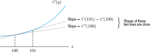
Figure 2.49: Marginal cost: Slope of one of these lines
there. Therefore, the average rate of change is close to the instantaneous rate of change. Since these rates of change are not very different, many economists choose to define marginal cost, MC, as the instantaneous rate of change of cost with respect to quantity:
![]()
Marginal cost is represented by the slope of the cost curve.
Similarly if the revenue generated by q flights is R(q) and the number of flights increases from 100 to 101, then
![]()
Now R(101) − R(100) is the average rate of change of revenue between 100 and 101 flights. As before, the average rate of change is approximately equal to the instantaneous rate of change, so economists often define
![]()
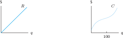
| Example 2 | If C(q) and R(q) for the airline are given in Figure 2.50, should the company add the 101st flight? |
| Solution | The marginal revenue is the slope of the revenue curve at q = 100. The marginal cost is the slope of the graph of C at q = 100. Figure 2.50 suggests that the slope at point A is smaller than the slope at B, so MC < MR for q = 100. This means that the airline will make more in extra revenue than it will spend in extra costs if it runs another flight, so it should go ahead and run the 101st flight. |

| Example 3 | The graph of a cost function is given in Figure 2.51. Does it cost more to produce the 500th item or the 2000th? Does it cost more to produce the 3000th item or the 4000th? At approximately what production level is marginal cost smallest? What is the total cost at this production level?
Figure 2.51: Estimating marginal cost: Where is marginal cost smallest? |
| Solution | The cost to produce an additional item is the marginal cost, which is represented by the slope of the cost curve. Since the slope of the cost function in Figure 2.51 is greater at q = 0.5 (when the quantity produced is 0.5 thousand, or 500) than at q = 2, it costs more to produce the 500th item than the 2000th item. Since the slope is greater at q = 4 than q = 3, it costs more to produce the 4000th item than the 3000th item.
The slope of the cost function is close to zero at q = 2, and is positive everywhere else, so the slope is smallest at q = 2. The marginal cost is smallest at a production level of 2000 units. Since C(2) ≈ 10,000, the total cost to produce 2000 units is about $10,000. |

| Example 4 | If the revenue and cost functions, R and C, are given by the graphs in Figure 2.52, sketch graphs of the marginal revenue and marginal cost functions, MR and MC.
|
| Solution | The revenue graph is a line through the origin, with equation
where p represents the constant price, so the slope is p and
The total cost is increasing, so the marginal cost is always positive. For small q values, the graph of the cost function is concave down, so the marginal cost is decreasing. For larger q, say q > 100, the graph of the cost function is concave up and the marginal cost is increasing. Thus, the marginal cost has a minimum at about q = 100. (See Figure 2.53.) |

Problems for Section 2.5
1. It costs $4800 to produce 1295 items and it costs $4830 to produce 1305 items. What is the approximate marginal cost at a production level of 1300 items?
2. The function C(q) gives the cost in dollars to produce q barrels of olive oil.
(a) What are the units of marginal cost?
(b) What is the practical meaning of the statement MC = 3 for q = 100?
3. In Figure 2.54, estimate the marginal revenue when the level of production is 600 units and interpret it.

4. In Figure 2.55, is marginal cost greater at q = 5 or at q = 30? At q = 20 or at q = 40? Explain.

5. In Figure 2.56, estimate the marginal cost when the level of production is 10,000 units and interpret it.

6. For q units of a product, a manufacturer's cost is C(q) dollars and revenue is R(q) dollars, with C(500) = 7200, R(500) = 9400, MC(500) = 15, and MR(500) = 20.
(a) What is the profit or loss at q = 500?
(b) If production is increased from 500 to 501 units, by approximately how much does profit change?
7. The cost of recycling q tons of paper is given in the following table. Estimate the marginal cost at q = 2000. Give units and interpret your answer in terms of cost. At approximately what production level does marginal cost appear smallest?
8. Figure 2.57 shows part of the graph of cost and revenue for a car manufacturer. Which is greater, marginal cost or marginal revenue, at
(a) q1?
(b) q2?

9. Let C(q) represent the total cost of producing q items. Suppose C(15) = 2300 and C′(15) = 108. Estimate the total cost of producing: (a) 16 items (b) 14 items.
10. To produce 1000 items, the total cost is $5000 and the marginal cost is $25 per item. Estimate the costs of producing 1001 items, 999 items, and 1100 items.
11. Let C(q) represent the cost and R(q) represent the revenue, in dollars, of producing q items.
(a) If C(50) = 4300 and C′(50) = 24, estimate C(52).
(b) If C′(50) = 24 and R′(50) = 35, approximately how much profit is earned by the 51st item?
(c) If C′(100) = 38 and R′(100) = 35, should the company produce the 101st item? Why or why not?
12. Cost and revenue functions for a charter bus company are shown in Figure 2.58. Should the company add a 50th bus? How about a 90th? Explain your answers using marginal revenue and marginal cost.

13. An industrial production process costs C(q) million dollars to produce q million units; these units then sell for R(q) million dollars. If C(2.1) = 5.1, R(2.1) = 6.9, MC(2.1) = 0.6, and MR(2.1) = 0.7, calculate
(a) The profit earned by producing 2.1 million units
(b) The approximate change in revenue if production increases from 2.1 to 2.14 million units.
(c) The approximate change in revenue if production decreases from 2.1 to 2.05 million units.
(d) The approximate change in profit in parts (b) and (c).
14. A company's cost of producing q liters of a chemical is C(q) dollars; this quantity can be sold for R(q) dollars. Suppose C(2000) = 5930 and R(2000) = 7780.
(a) What is the profit at a production level of 2000?
(b) If MC(2000) = 2.1 and MR(2000) = 2.5, what is the approximate change in profit if q is increased from 2000 to 2001? Should the company increase or decrease production from q = 2000?
(c) If MC(2000) = 4.77 and MR(2000) = 4.32, should the company increase or decrease production from q = 2000?
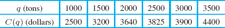
15. Table 2.13 shows the cost, C(q), and revenue, R(q), in terms of quantity q. Estimate the marginal cost, C′(q), and marginal revenue, R′(q), for q between 0 and 7.

16. Table 2.14 shows the cost, C(q), and revenue, R(q), in terms of quantity q. Estimate the marginal cost, MC(q), and marginal revenue, MR(q), for q between 0 and 6.

CHAPTER SUMMARY
- Rate of change
Average, instantaneous
- Estimating derivatives
Estimate derivatives from a graph, table of values, or formula
- Interpretation of derivatives
Rate of change, slope, using units, instantaneous velocity
- Relative rate of change
Calculation and interpretation
- Marginality
Marginal cost and marginal revenue
- Second derivative
Concavity
- Derivatives and graphs
Understand relation between sign of f′ and whether f is increasing or decreasing. Sketch graph of f′ from graph of f. Marginal analysis
REVIEW PROBLEMS FOR CHAPTER TWO
1. In a time of t seconds, a particle moves a distance of s meters from its starting point, where s = 3t2.
(a) Find the average velocity between t = 1 and t = 1 + h if:
(i) h = 0.1, (ii) h = 0.01, (iii) h = 0.001.
(b) Use your answers to part (a) to estimate the instantaneous velocity of the particle at time t = 1.
2. Figure 2.59 shows the graph of f. Match the derivatives in the table with the points a, b, c, d, e.


3. (a) Use a graph of f(x) = 2 − x3 to decide whether f′(1) is positive or negative. Give reasons.
(b) Use a small interval to estimate f′(1).
4. Estimate f′(2) for f(x) = 3x. Explain your reasoning.
5. (a) The function f is given in Figure 2.60. At which of the labeled points is f′(x) positive? Negative? Zero?
(b) At which labeled point is f′ largest? At which labeled point is f′ most negative?

6. Use Figure 2.61 to fill in the blanks in the following statements about the function g at point B.
(a) g(__)=__
(b) g′(__)=__

7. In a time of t seconds, a particle moves a distance of s meters from its starting point, where s = sin(2t).
(a) Find the average velocity between t = 1 and t = 1 + h if:
(i) h = 0.1, (ii) h = 0.01, (iii) h = 0.001.
(b) Use your answers to part (a) to estimate the instantaneous velocity of the particle at time t = 1.
8. The distance (in feet) of an object from a point is given by s(t) = t2, where time t is in seconds.
(a) What is the average velocity of the object between t = 3 and t = 5?
(b) By using smaller and smaller intervals around 3, estimate the instantaneous velocity at time t = 3.
9. Let f(x) = 5x. Use small intervals to estimate f′(2).
10. Using slopes to left and right of 0, estimate P′(0) if P(t) = 200(1.05)t.
Sketch the graphs of the derivatives of the functions shown in Problems 11–20. Be sure your sketches are consistent with the important features of the graphs of the original functions.
11.

12.
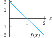
13.

14.

15.

16.

17.

18.

19.

20.

21. (a) Estimate f′(2) using the values of f in the table.
(b) For what values of x does f′(x) appear to be positive? Negative?
![]()
22. Figure 2.62 is the graph of f′, the derivative of a function f. On what interval(s) is the function f
(a) Increasing?
(b) Decreasing?

Figure 2.62: Graph of f′, not f
23. The average weight W of an oak tree in kilograms that is x meters tall is given by the function W = f(x). What are the units of measurement of f′(x)?
24. The percent, P, of US households with a personal computer is a function of the number of years, t, since 1982 (when the percent was essentially zero), so P = f(t). Interpret the statements f(20) = 57 and f′(20) = 3.
25. The temperature, T, in degrees Fahrenheit, of a cold yam placed in a hot oven is given by T = f(t), where t is the time in minutes since the yam was put in the oven.
(a) What is the sign of f′(t)? Why?
(b) What are the units of f′(20)? What is the practical meaning of the statement f′(20) = 2?
26. The quantity sold, q, of a certain product is a function of the price, p, so q = f(p). Interpret each of the following statements in terms of demand for the product:
(a) f(15) = 200
(b) f′(15) = −25.
27. Figure 2.63 shows the length, L, in cm, of a sturgeon (a type of fish) as a function of the time, t, in years.29 Estimate f′(10). Give units and interpret your answer.

28. Suppose that f(x) is a function with f(20) = 345 and f′(20) = 6. Estimate f(22).
29. The wind speed W in meters per second at a distance x kilometers from the center of a hurricane is given by the function W = h(x). What does the fact that h′(15) > 0 tell you about the hurricane?
30. You drop a rock from a high tower. After it falls x meters its speed S in meters per second is S = h(x). What is the meaning of h′(20) = 0.5 ?
31. If t is the number of years since 2011, the population, P, of China, in billions, can be approximated by the function
![]()
Estimate f(9) and f′(9), giving units. What do these two numbers tell you about the population of China?
32. After investing $1000 at an annual interest rate of 7% compounded continuously for t years, your balance is $B, where B = f(t). What are the units of dB/dt? What is the financial interpretation of dB/dt?
33. Let f(t) be the depth, in centimeters, of water in a tank at time t, in minutes.
(a) What does the sign of f′(t) tell us?
(b) Explain the meaning of f′(30) = 20. Include units.
(c) Using the information in part (b), at time t = 30 minutes, find the rate of change of depth, in meters, with respect to time in hours. Give units.
34. For the function graphed in Figure 2.64, are the following nonzero quantities positive or negative?
(a) f(2)
(b) f′(2)
(c) f″(2)

35. At one of the labeled points on the graph in Figure 2.65 both dy/dx and d2y/dx2 are positive. Which is it?

36. A climber on Mount Everest is 6000 meters from the start of a trail and at elevation 8000 meters above sea level. At x meters from the start, the elevation of the trail is h(x) meters above sea level. If h′(x) = 0.5 for x near 6000, what is the approximate elevation another 3 meters along the trail?
37. Let f(v) be the gas consumption (in liters/km) of a car going at velocity v (in km/hr). In other words, f(v) tells you how many liters of gas the car uses to go one kilometer at velocity v. Explain what the following statements tell you about gas consumption:
![]()
38. To study traffic flow, a city installs a device which records C(t), the total number of cars that have passed by t hours after 4:00 am. The graph of C(t) is in Figure 2.66.
(a) When is the traffic flow the greatest?
(b) Estimate C′(2).
(c) What does C′(2) mean in practical terms?

39. The temperature, H, in degrees Celsius, of a cup of coffee placed on the kitchen counter is given by H = f(t), where t is in minutes since the coffee was put on the counter.
(a) Is f′(t) positive or negative? Give a reason for your answer.
(b) What are the units of f′(20)? What is its practical meaning in terms of the temperature of the coffee?
40. Suppose that f(x) is a function with f(100) = 35 and f′(100) = 3. Estimate f(102).
41. Suppose P(t) is the monthly payment, in dollars, on a mortgage which will take t years to pay off. What are the units of P′(t)? What is the practical meaning of P′(t)? What is its sign?
42. The population, P, of a city (in thousands) at time t (in years) is P = 700e0.035t. Estimate the relative rate of change of the population at t = 3 using
(a) Δt = 1
(b) Δt = 0.1
(c) Δt = 0.01
43. For each part below, sketch a graph of a function that satisfies the given conditions. There are many possible correct answers.
(a) f′ > 0 and f″ > 0.
(b) f′ > 0 and f″ < 0.
(c) f′ < 0 and f″ > 0.
(d) f′ < 0 and f″ < 0.
44. For each function, do the signs of the first and second derivatives of the function appear to be positive or negative over the given interval?
(a)

(b)

(c)

45. The length L of the day in minutes (sunrise to sunset) x kilometers north of the equator on June 21 is given by L = f(x). What are the units of
(a) f′(3000)?
(b) f″(3000)?
46. Sketch the graph of a function whose first and second derivatives are everywhere positive.
47. At which of the marked x-values in Figure 2.67 can the following statements be true?
(a) f(x) < 0
(b) f′(x) < 0
(c) f(x) is decreasing
(d) f′(x) is decreasing
(e) Slope of f(x) is positive
(f) Slope of f(x) is increasing

48. Sketch the graph of the height of a particle against time if velocity is positive and acceleration is negative.
49. Figure 2.68 gives the position, f(t), of a particle at time t. At which of the marked values of t can the following statements be true?
(a) The position is positive
(b) The velocity is positive
(c) The acceleration is positive
(d) The position is decreasing
(e) The velocity is decreasing

50. A high school principal is concerned about the drop in the percentage of students who graduate from her school, shown in the following table, compared with the fall in national average from 69.2% in 2006 to 68.8% in 2007.30

(a) Calculate the average rate of change of P for each of the three-year intervals between 1995 and 2007.
(b) Does d2P/dt2 appear to be positive or negative between 1995 and 2007?
(c) Explain why the values of P and dP/dt are trouble-some to the principal.
(d) Explain why the sign of d2P/dt2 and the magnitude of dP/dt in the year 2004 may give the principal some cause for optimism.
51. Students were asked to evaluate f′(4) from the following table which shows values of the function f:

- Student A estimated the derivative as f′(4) ≈
- Student B estimated the derivative as f′(4) ≈

- Student C suggested that they should split the difference and estimate the average of these two results, that is, f′(4) ≈
 (0.5 + 0.3) = 0.4.
(a) Sketch the graph of f, and indicate how the three estimates are represented on the graph.
(b) Explain which answer is likely to be best.
52. Figure 2.69 shows the rate at which energy, f(v), is consumed by a bird flying at speed v meters/sec.
(a) What rate of energy consumption is needed by the bird to keep aloft, without moving forward?
(b) What does the shape of the graph tell you about how birds fly?
(c) Sketch f′(v).

STRENGTHEN YOUR UNDERSTANDING
In Problems 1–55, indicate whether the statement is true or false.
1. The derivative of f at a is the instantaneous rate of change of f at the point a.
2. If f(x) = x2 then f′(1) is positive.
3. If g(t) = 2t then g′(1) ≈ (21.001 − 21)/(1.001 − 1).
4. The slope of the graph of H(x) = ![]() is negative at x = 2.
is negative at x = 2.
5. A function f cannot have both f(a) = 0 and f′(a) = 0.
6. The average rate of change of f between 0 and 1 is always less than the slope of the graph of f at 0.
7. The function r in the following table appears to have a negative derivative at t = 0.5:

8. The derivative of f at 3 is given by the difference quotient (f(3) − f(0))/(3 − 0).
9. If R(w) = w3 then R′(−2) is negative.
10. A function can have more than one point where the derivative is 0.
11. If f′ > 0 on an interval, then f is increasing on that interval.
12. The f is negative on an interval, then the derivative of f is decreasing on that interval.
13. If f is always increasing, then f′ is always increasing.
14. If f(2) > g(2) then f′(2) > g′(2).
15. The derivative of the constant function q(x) = 5 is q′(x) = 0.
16. The derivative of a function that is always decreasing is also always decreasing.
17. The function g(t) = ln(t) has g′(1) < 0.
18. If f is a function with f(3) = 0 then f′(3) = 0.
19. If f′ is zero at all points in an interval, then the graph of f is a horizontal line on that interval.
20. If f′ is negative at all points in an interval, then f is decreasing on that interval.
21. If the cost C (in dollars) of feeding x students in the dining center is given by C = f(x), then the units of dC/dx are dollars per student.
22. If y = f(x) then dy/dx and f′(x) mean the same thing.
23. If the cost C (in dollars) of extracting T tons of ore is given by C = f(T) then f′(2000) is the approximate cost to extract the 2001st ton.
24. If f(10) = 20 and f′(10) = 3, then 23 is a reasonable approximation of f(11).
25. The units of dA/dB are the units of A divided by the units of B.
26. If A = f(B) then the units of f′(B) are the units of B divided by the units of A.
27. If f′(100) = 2 and the derivative of f is not changing rapidly, then f(101) − f(100) ≈ 2.
28. If t (in minutes) is the time that a dose of D milligrams of morphine is effective as a painkiller, so that t = f(D), then the units of f′(D) are minutes per milligram.
29. If h = f(a) gives height h (in inches) of a child aged a years, then dh/da is positive when 0 < a < 10.
30. If W = f(R) and f′(R) is negative, then we expect W to decrease as R increases.
31. If f″ > 0 on an interval, then f is increasing on that interval.
32. If f″ < 0 on an interval, then f is concave down on that interval.
33. If f″ > 0 on an interval, then f′ > 0 on that interval.
34. If f′ is decreasing on an interval, then f is concave down on that interval.
35. If a car is slowing down, then the second derivative of its distance as a function of time is negative.
36. There is a function with f > 0 and f′ > 0 and f″ > 0 everywhere.
37. There is a function with f > 0 and f′ < 0 and f″ > 0 everywhere.
38. There is a function with f″ = 0 everywhere.
39. The function f(x) = ex has f″ > 0 everywhere.
40. The function f(x) = ln(x) has f″ > 0 for x > 0.
41. Marginal cost is the instantaneous rate of change of cost with respect to quantity.
42. Marginal revenue is the derivative of the revenue function with respect to quantity.
43. If marginal revenue is greater than marginal cost when quantity is 1000, then increasing the quantity to 1001 will increase the profit.
44. Marginal cost is always greater than or equal to zero.
45. If the revenue function is linear with slope 5, then marginal revenue is always zero.
46. The units of marginal cost are quantity per dollar.
47. The units of marginal revenue are the same as the units of marginal cost.
48. Marginal cost is never equal to marginal revenue.
49. If the graphs of the cost and revenue functions C(q) and R(q) cross at q*, then marginal revenue is equal to marginal cost at q*.
50. If the graphs of the marginal cost and marginal revenue functions C′(q) and R′(q) cross at q*, then marginal revenue is equal to marginal cost at q*.
51. If P is a function of t, then the relative rate of change of P is (1/P)(dP/dt).
52. If f(25) = 10 gallons and f′(25) = 2 gallons per minute, then at t = 25, the function f is changing at a rate of 20% per minute.
53. If a quantity is 100 and has relative rate of change −3% per minute, we expect the quantity to be about 97 one minute later.
54. If a population of animals changes from 500 to 400 in one month, then the relative rate of change is about −100 animals per month.
55. Linear functions have constant rate of change and exponential functions have constant relative rate of change.
PROJECTS FOR CHAPTER TWO
1. Estimating the Temperature of a Yam
You put a yam in a hot oven, maintained at a constant temperature of 200°C. As the yam picks up heat from the oven, its temperature rises.31
(a) Draw a possible graph of the temperature T of the yam against time t (minutes) since it is put into the oven. Explain any interesting features of the graph, and in particular explain its concavity.
(b) At t = 30, the temperature T of the yam is 120° and increasing at the (instantaneous) rate of 2°/min. Using this information and the shape of the graph, estimate the temperature at time t = 40.
(c) In addition, you are told that at t = 60, the temperature of the yam is 165°. Can you improve your estimate of the temperature at t = 40?
(d) Assuming all the data given so far, estimate the time at which the temperature of the yam is 150°.
2. Temperature and Illumination
Alone in your dim, unheated room, you light a single candle rather than curse the darkness. Depressed with the situation, you walk directly away from the candle, sighing. The temperature (in degrees Fahrenheit) and illumination (in % of one candle power) decrease as your distance (in feet) from the candle increases. In fact, you have tables showing this information.


You are cold when the temperature is below 40°. You are in the dark when the illumination is at most 50% of one candle power.
(a) Two graphs are shown in Figures 2.70 and 2.71. One is temperature as a function of distance and one is illumination as a function of distance. Which is which? Explain.


(b) What is the average rate at which the temperature is changing when the illumination drops from 75% to 56%?
(c) You can still read your watch when the illumination is about 65%. Can you still read your watch at 3.5 feet? Explain.
(d) Suppose you know that at 6 feet the instantaneous rate of change of the temperature is −4.5°F/ft and the instantaneous rate of change of illumination is −3% candle power/ft. Estimate the temperature and the illumination at 7 feet.
(e) Are you in the dark before you are cold, or vice versa?
3. Chlorofluorocarbons (CFCs) in the Atmosphere
Chlorofluorocarbons (CFCs) were used as propellants in spray cans until their buildup in the atmosphere started destroying the ozone, which protects us from ultraviolet rays. Since the 1987 Montreal Protocol (an agreement to curb CFCs), the CFCs in the atmosphere above the US have been reduced from a high of 3200 parts per trillion (ppt) in 1994 to 2750 ppt in 2010.32 The reduction has been approximately linear. Let C(t) be the concentration of CFCs in ppt in year t.
(a) Find C(1994) and C(2010).
(b) Estimate C′(1994) and C′(2010).
(c) Assuming C(t) is linear, find a formula for C(t).
(d) When is C(t) expected to reach 1850 ppt, the level before CFCs were introduced?
(e) If you were told that in the future, C(t) would not be exactly linear, and that C″(t) > 0, would your answer to part (d) be too early or too late?
FOCUS ON THEORY
LIMITS, CONTINUITY, AND THE DEFINITION OF THE DERIVATIVE
The velocity at a single instant in time is surprisingly difficult to define precisely. Consider the statement “At the instant it crossed the finish line, the horse was traveling at 42 mph.” How can such a claim be substantiated? A photograph taken at that instant will show the horse motionless—it is no help at all. There is some paradox in trying to quantify the property of motion at a particular instant in time, since by focusing on a single instant we stop the motion!
A similar difficulty arises whenever we attempt to measure the rate of change of anything—for example, oil leaking out of a damaged tanker. The statement “One hour after the ship's hull ruptured, oil was leaking at a rate of 200 barrels per second” seems not to make sense. We could argue that at any given instant no oil is leaking.
Problems of motion were of central concern to Zeno and other philosophers as early as the fifth century BC. The approach that we took, made famous by Newton's calculus, is to stop looking for a simple notion of speed at an instant, and instead to look at speed over small intervals containing the instant. This method sidesteps the philosophical problems mentioned earlier but brings new ones of its own.
Definition of the Derivative Using Average Rates
In Section 2.1, we defined the derivative as the instantaneous rate of change of a function. We can estimate a derivative by computing average rates of change over smaller and smaller intervals. We use this idea to give a symbolic definition of the derivative. Letting h represent the size of the interval, we have

To find the derivative, or instantaneous rate of change at the point x, we use smaller and smaller intervals. To find the derivative exactly, we take the limit as h, the size of the interval, shrinks to zero, so we say
![]()
Finally, instead of writing the phrase “limit, as h approaches 0,” we use the notation ![]() . This leads to the following symbolic definition:
. This leads to the following symbolic definition:
For any function f, we define the derivative function, f′, by
![]()
provided the limit exists. The function f is said to be differentiable at any point x at which the derivative function is defined.
Notice that we have replaced the original difficulty of computing velocity at a point by an argument that the average rates of change approach a number as the time intervals shrink in size. In a sense, we have traded one hard question for another, since we don't yet have any idea how to be certain what number the average velocities are approaching.
The Idea of a Limit
We used a limit to define the derivative. Now we look a bit more at the idea of the limit of a function at the point c. Provided the limit exists:
We write ![]() f(x) to represent the number approached by f(x) as x approaches c.
f(x) to represent the number approached by f(x) as x approaches c.
| Example 1 | Investigate |
| Solution | Notice that we can make x2 as close to 4 as we like by taking x sufficiently close to 2. (Look at the values of 1.92, 1.992, 1.9992, and 2.12, 2.012, 2.0012 in Table 2.15; they seem to be approaching 4.) We write
which is read “the limit, as x approaches 2, of x2 is 4.” Notice that the limit does not ask what happens at x = 2, so it is not sufficient to substitute 2 to find the answer. The limit describes behavior of a function near a point, not at the point. |
| Example 2 | Use a graph to estimate
|
| Solution | Notice that the expression
|

| Example 3 | Estimate |
| Solution | The limit is the value approached by this expression as h approaches 0. The values in Table 2.16 seem to be approaching 6 as h → 0. So it is a reasonable guess that
However, we cannot be sure that the limit is exactly 6 by looking at the table. To calculate the limit exactly requires algebra. |
| Example 4 | Use algebra to find |
| Solution | Expanding the numerator gives
Since taking the limit as h → 0 means looking at values of h near, but not equal, to 0, we can cancel a common factor of h, giving
As h approaches 0, the values of (6 + h) approach 6, so
|
Continuity
Roughly speaking, a function is said to be continuous on an interval if its graph has no breaks, jumps, or holes in that interval. A continuous function has a graph that can be drawn without lifting the pencil from the paper.
Example: The function f(x) = 3x2 − x2 + 2x + 1 is continuous on any interval. (See Figure 2.73.)
Example: The function f(x) = 1/x is not defined at x = 0. It is continuous on any interval not containing the origin. (See Figure 2.74.)
Example: Suppose p(x) is the price of mailing a first-class letter weighing x ounces. It costs 46¢ for one ounce or less, 66¢ between the first and second ounces, and so on. So the graph (in Figure 2.75) is a series of steps. This function is not continuous on intervals such as (0,2) because the graph jumps at x = 1.

Figure 2.73: The graph of f(x) = 3x3 − x2 + 2x − 1
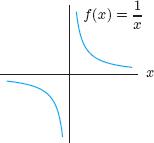
Figure 2.74: Graph of f(x) = 1/x: Not defined at 0

Figure 2.75: Cost of mailing a letter
What Does Continuity Mean Numerically?
Continuity is important in practical work because it means that small errors in the independent variable lead to small errors in the value of the function.
Example: Suppose that f(x) = x2 and that we want to compute f(π). Knowing f is continuous tells us that taking x = 3.14 should give a good approximation to f(π), and that we can get a better approximation to f(π) by using more decimals of π.
Example: If p(x) is the cost of mailing a letter weighing x ounces, then p(0.99) = p(1) = 46¢, whereas p(1.01) = 66¢, because as soon as we get over 1 ounce, the price jumps up to 66¢. So a small difference in the weight of a letter can lead to a significant difference in its mailing cost. Hence p is not continuous at x = 1.
Definition of Continuity
We now define continuity using limits. The idea of continuity rules out breaks, jumps, or holes by demanding that the behavior of a function near a point be consistent with its behavior at the point:
The function f is continuous at x = c if f is defined at x = c and
![]()
The function is continuous on an interval (a, b) if it is continuous at every point in the interval.
Which Functions Are Continuous?
Requiring a function to be continuous on an interval is not asking very much, as any function whose graph is an unbroken curve over the interval is continuous. For example, exponential functions, polynomials, and sine and cosine are continuous on every interval. Functions created by adding, multiplying, or composing continuous functions are also continuous.
Using the Definition to Calculate Derivatives
By estimating the derivative of the function f(x) = x2 at several points, we guessed in Example 5 of Section 2.2 that the derivative of x2 is f′(x) = 2x. In order to show that this formula is correct, we have to use the symbolic definition of the derivative given earlier in this section.
In evaluating the expression
![]()
we simplify the difference quotient first, and then take the limit as h approaches zero.
| Example 5 | Show that the derivative of f(x) = x2 is f′(x) = 2x. |
| Solution | Using the definition of the derivative with f(x) = x2, we have
To take the limit, look at what happens when h is close to 0, but do not let h = 0. Since h ≠ 0, we cancel the common factor of h, giving
because as h gets close to zero, 2x + h gets close to 2x. So
|
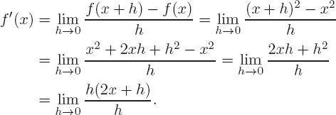

Problems on Limits and the Definition of the Derivative
1. On Figure 2.76, mark lengths that represent the quantities in parts (a) − (e). (Pick any h, with h > 0.)
(a) a + h
(b) h
(c) f(a)
(d) f(a + h)
(e) f(a + h)−f(a)
(f) Using your answers to parts (a)–(e), show how the quantity ![]() can be represented as the slope of a line on the graph.
can be represented as the slope of a line on the graph.
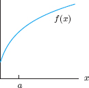
2. On Figure 2.77, mark lengths that represent the quantities in parts (a)–(e). (Pick any h, with h > 0.)
(a) a + h
(b) h
(c) f(a)
(d) f(a + h)
(e) f(a+h)–f(a)
(f) Using your answers to parts (a)–(e), represent the quantity ![]() as the slope of a line on the graph.
as the slope of a line on the graph.

For the expressions in Problems 3–6,
(a) What is the result when we substitute h = 0?
(b) Find the values when we substitute h = 0.1, h = 0.01, h = 0.001, and h = 0.0001.
(c) Use the results of part (b) to estimate the limit as h goes to zero.
3. ![]()
4. ![]()
5. ![]()
6. ![]()
Use a graph to estimate the limits in Problems 7–8.
7. ![]()
8. ![]() (with x in radians)
(with x in radians)
Estimate the limits in Problems 9–12 by substituting smaller and smaller values of h. For trigonometric functions, use radians. Give answers to one decimal place.
10. ![]()
11. ![]()
12. ![]()
In Problems 13–16, does the function f(x) appear to be continuous on the interval 0 ≤ x ≤ 2? If not, what about on the interval 0 ≤ x ≤ 0.5?
13.

14.

15.

16.

17. The graph of y = f(x) is in Figure 2.78. Does the function f(x) appear to be continuous on the given interval?
(a) 1 ≤ x ≤ 3
(b) 0.5 ≤ x ≤ 1.5
(c) 3 ≤ x ≤ 5
(d) 2 ≤ x ≤ 6


18. The graph of y = f(x) is in Figure 2.79. Does the function f(x) appear to be continuous on the given interval?
(a) 1 ≤ x ≤ 3
(b) 0.5 ≤ x ≤ 1.5
(c) 3 ≤ x ≤ 5
(d) 4 ≤ x ≤ 5
In Problems 19–22, find the limit by simplifying the expression.
19. ![]()
20. ![]()
21. ![]()
22. ![]()
Are the functions in Problems 23–28 continuous on the given intervals?
23. f(x) = x + 2 on −3 ≤ x ≤ 3
24. f(x) = 2x on 0 ≤ x ≤ 10
25. f(x) = x2 + 2 on 0 ≤ x ≤ 5
26. f(x) = ![]() on 2 ≤ x ≤ 3
on 2 ≤ x ≤ 3
27. f(x) = ![]() on 0 ≤ x ≤ 2
on 0 ≤ x ≤ 2
28. f(x) = ![]() on 0 ≤ x ≤ 2
on 0 ≤ x ≤ 2
Which of the functions described in Problems 29–33 are continuous?
29. The number of people in a village as a function of time.
30. The distance traveled by a car in stop-and-go traffic as a function of time.
31. The weight of a baby as a function of time during the second month of the baby's life.
32. The number of pairs of pants as a function of the number of yards of cloth from which they are made. Each pair requires 3 yards.
33. You start in North Carolina and go westward on Interstate 40 toward California. Consider the function giving the local time of day as a function of your distance from your starting point.
Use the definition of the derivative to show how the formulas in Problems 34–43 are obtained.
34. If f(x) = 5x, then f′(x) = 5.
35. If f(x) = 3x − 2, then f′(x) = 3.
36. If f(x) = x2 + 4, then f′(x) = 2x.
37. If f(x) = 3x2, then f′(x) = 6x.
38. If f(x) = x − x2, then f′(x) = 1 − 2x.
39. If f(x) = 5x2 + 1, then f′(x) = 10x.
40. If f(x) = 2x2 + x, then f′(x) = 4x + 1.
41. If f(x) = −2x3, then f′(x) = −6x2.
42. If f(x) = 1 − x3, then f′(x) = −3x2.
43. If f(x) = 1/x, then f′(x) = −1/x2.
1Statistical Abstracts of the United States 2004–2005, Table 796.
2www.nass.usda.gov:81/ipedb/farmnum.htm, accessed April 11, 2005.
3http://www.prb.org/Publications/Datasheets/2010/2010wpds, accessed September 2012.
4http://2010.census.gov/2010census/, accessed September 2012.
5Statistical Abstracts of the US, 1985, US Department of Commerce, Bureau of the Census, p. 22, and http://www.census.gov/compendia/statab/cats/population/estimates_and_projections–states_metropolitan_areas_cities.html, accessed September 2012.
6The World Almanac and Book of Facts 2005, p. 151 (New York). Production workers include nonsupervisory workers in mining, manufacturing, construction, transportation, public utilities, wholesale and retail trade, finance, insurance, real estate, and services.
7“State-conditional fertilizer yield response on western Kenyan farms”, by P. Marenya, C. Barrett, Social Science Research Network, abstract = 1141937, 2009.
8en.wikipedia.org/wiki/Photovoltaics. Accessed February 2013. A gigawatt measures power and can be used to measure energy-generating capacity.
9The Worldwatch Institute, Vital Signs 2001, p. 47 (New York: W.W. Norton, 2001).
10Adapted from John B. West, Respiratory Physiology, 4th Ed. (New York: Williams and Wilkins, 1990).
11OC Register, May 9, 2007; The New York Times, May 14, 2007.
12http://minerals.usgs.gov/ds/2005/140/gold.pdf, accessed September 2012.
132008 Annual Report to Stockholders, accessed at www.thehersheycompany.com.
14http://www.fao.org/economic/ess/ess-publications/ess-yearbook/ess-yearbook2010/en/, accessed September 2012.
15www.climate.org/topics/sea-level, accessed June 5, 2011.
16www.rain-tree.com/facts.htm, accessed June 2009.
17www.facebook.com/press, accessed June 2009.
18www.census.gov/population/international/data/worldpop. Accessed February 2013.
19www.asymco.com/2011/07/13/itunes-app-total-downloads-finally-overtook-song-downloads/, accessed January 21, 2013.
20www.mjperry.blogspot.com/2011/11/ndakota-oil-continues-exponential.html, accessed January 21, 2013.
22In the Boston Globe, March 13, 1985, Representative William Gray (D–Pa.) was reported as saying: “It's confusing to the American people to imply that Congress threatens national security with reductions when you're really talking about a reduction in the increase.”
23Statistical Abstracts of the United States 2004–2009, Table 99.
24www.bts.gov/publications/national_transportation_statistics/html/table_01_ll.html. Accessed April 27, 2011.
25From Paul A. Samuelson, Economics, 11th edition (New York: McGraw-Hill, 1981).
26www.epa.gov/climatechange/effects/coastal/sap4-1.html, Coastal Sensitivity to Sea-Level Rise: A Focus on the Mid-Atlantic Region, US Climate Change Science Program, January 2009.
27www.internetworldstats.com/facebook.htm, accessed January 21, 2013.
28T. Carlson, “Über Geschwindigkeit und Grösse der Hefevermehrung in Würze”, Biochem. Z., 1913.
29Data from L. von Bertalanffy, General System Theory, p. 177 (New York: Braziller, 1968).
30http://www.csmonitor.com/USA/Education/2010/0610/Graduation-rate-for-US-high-schoolers-falls-for-second-straight-year, accessed September 2012.
31From Peter D. Taylor, Calculus: The Analysis of Functions (Toronto: Wall & Emerson, Inc., 1992).