Before we delve into the extended examples later in this book, you will require a Python environment and a working knowledge of TensorFlow. Therefore, this chapter will show you how to install a Python environment ready to run the code in this book. Once that’s in place, I’ll cover the basics of the TensorFlow machine-learning library.
How to Set Up Your Python Environment
All the code in this book was developed with the Python distribution Anaconda and Jupyter notebooks. To set up Anaconda, first download and install it for your operating system. (I used Windows 10, but the code is not dependent on this system. Feel free to use a version for Mac, if you prefer.) You may retrieve Anaconda by accessing https://anaconda.org/ .

On the Anaconda web site, at the top right of the page, you will find a link to download the required software

The screen you see when you start Anaconda
Python packages (like NumPy) are updated regularly and very often. It can happen that a new version of a package makes your code stop working. Functions are deprecated and removed, and new ones are added. To solve this problem, in Anaconda, you can create what is called an environment. This is basically a container that holds a specific Python version and specific versions of the packages you decide to install. With this, you can have a container for Python 2.7 and NumPy 1.10 and another with Python 3.6 and NumPy 1.13, for example. You may have to work with existing code that has been developed with Python 2.7, and, therefore, you must have a container with the right Python version. But, at the same time, it may be that you require Python 3.6 for your projects. With containers, you can ensure all this at the same time. Sometimes different packages conflict with each other, so you must be careful and avoid installing all packages you find interesting in your environment, especially if you are developing packages under a deadline. Nothing is worse than discovering that your code is no longer working, and you don’t know why.
Note
When you define an environment, try to install only the packages you really need, and pay attention when you update them, to make sure that any upgrade does not break your code. (Remember: Functions are deprecated, removed, added, or frequently changed.) Check the documentation of updates before upgrading, and do so only if you really need the updated features.
You can create an environment from the command line, using the conda command , but to get an environment up and running for our code, everything can be done from the graphical interface. This is the method I will explain here, because it is the easiest. I suggest that you read the following page on the Anaconda documentation, to understand in detail how to work within its environment: https://conda.io/docs/user-guide/tasks/manage-environments.html .
Creating an Environment
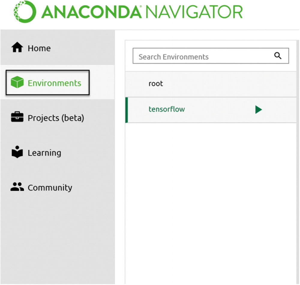
To create a new environment, you first must go into the Environments section of the application, by clicking the related link from the left navigation pane (indicated in the figure by a black rectangle)

To create a new environment, you must click the Create button (indicated with a plus sign) from the middle navigation pane. In the figure, a red arrow indicates the location of the button.
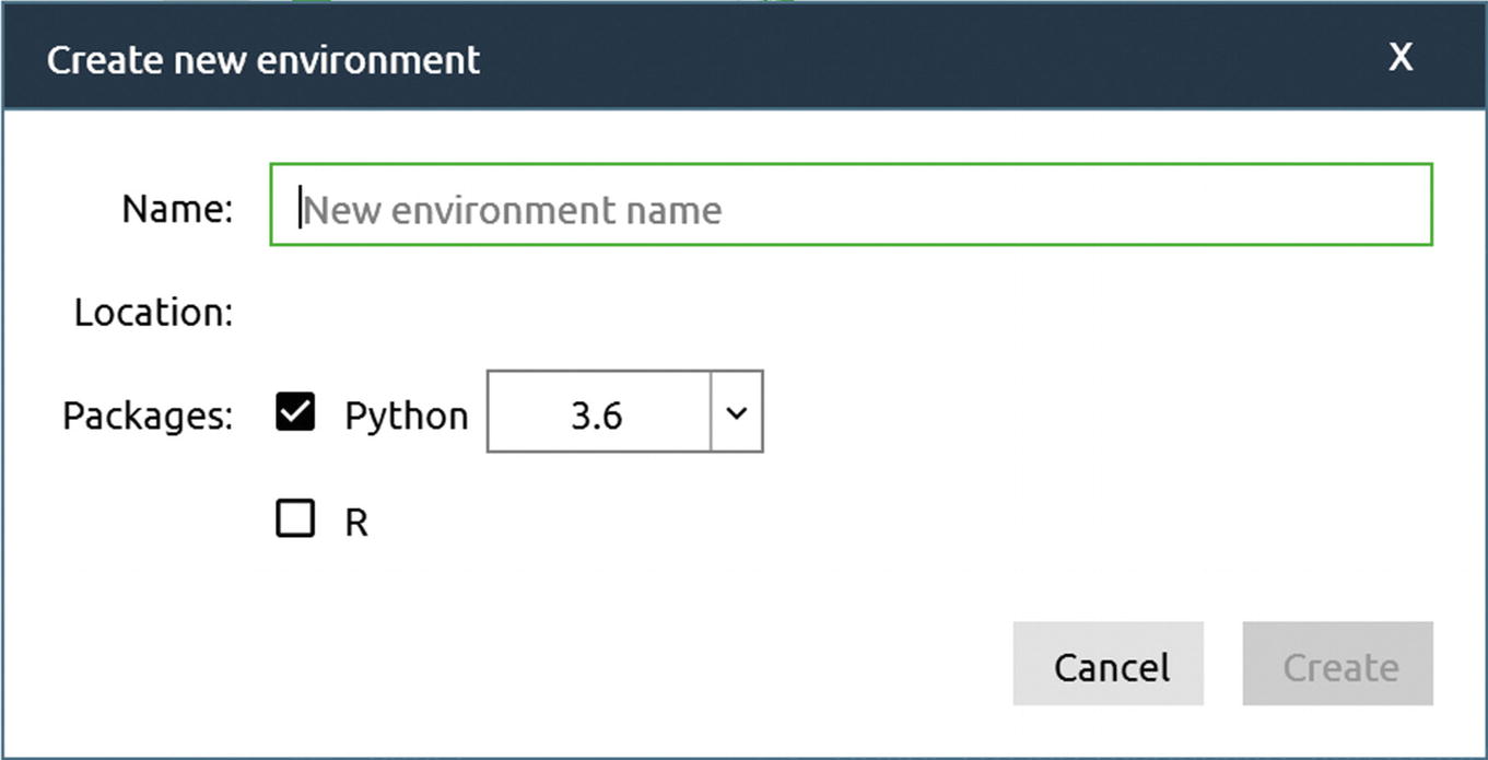
The window you will see when you click the Create button indicated in Figure 1-4
You can choose any name. In this book, I used the name tensorflow. As soon as you type a name, the Create button becomes active (and green). Click it and wait a few minutes until all the necessary packages are installed. Sometimes, you may get a pop-up window telling you that a new version of Anaconda is available and asking if you want to upgrade. Feel free to click yes. Follow the on-screen instructions until Anaconda navigator starts again, in the event you received this message and clicked yes.
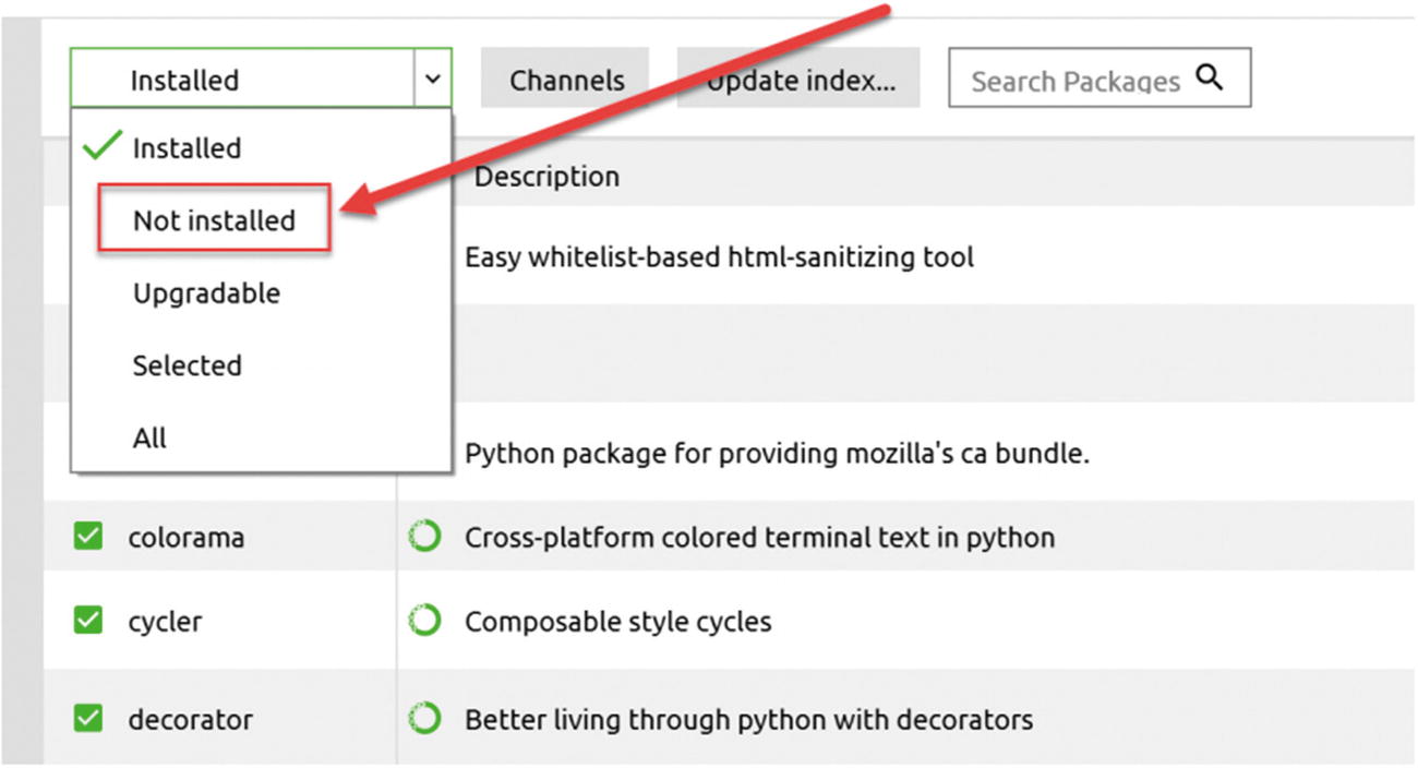
Selecting the Not installed value from the drop-down menu
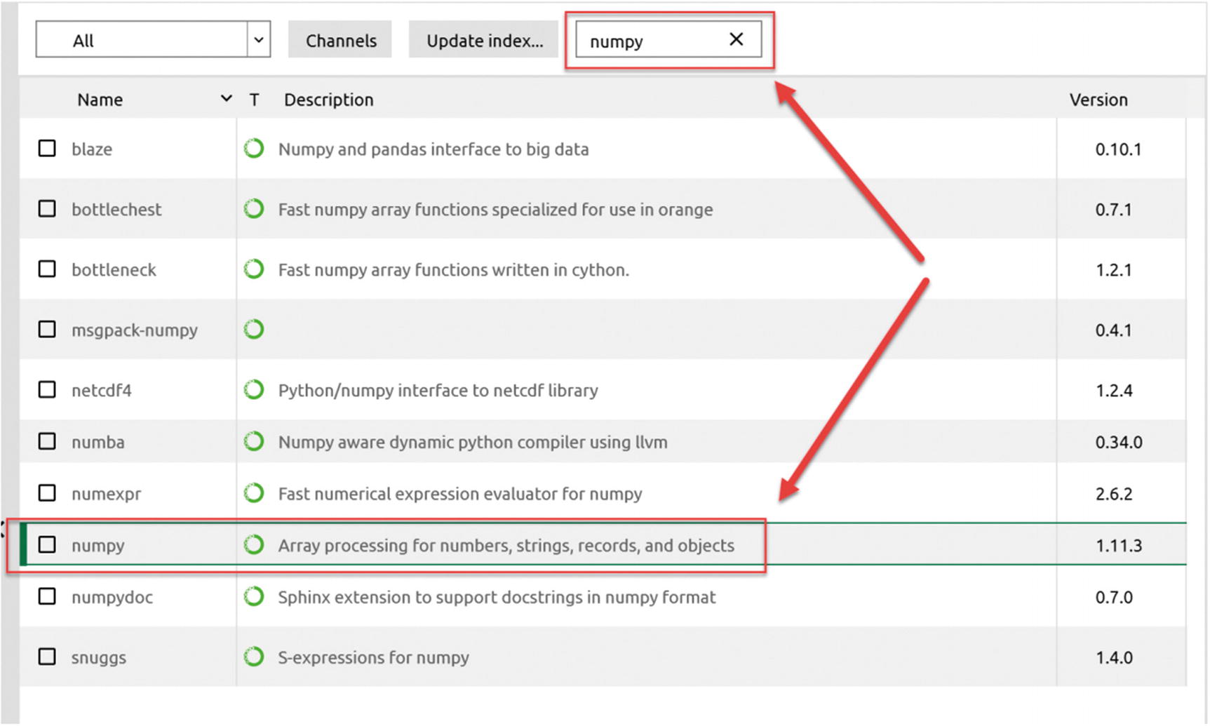
Type “numpy” in the search field, to include it in the package repository
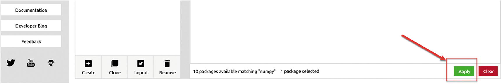
After you have selected the numpy package for installation, click the green Apply button. The button is at the lower right of the interface.
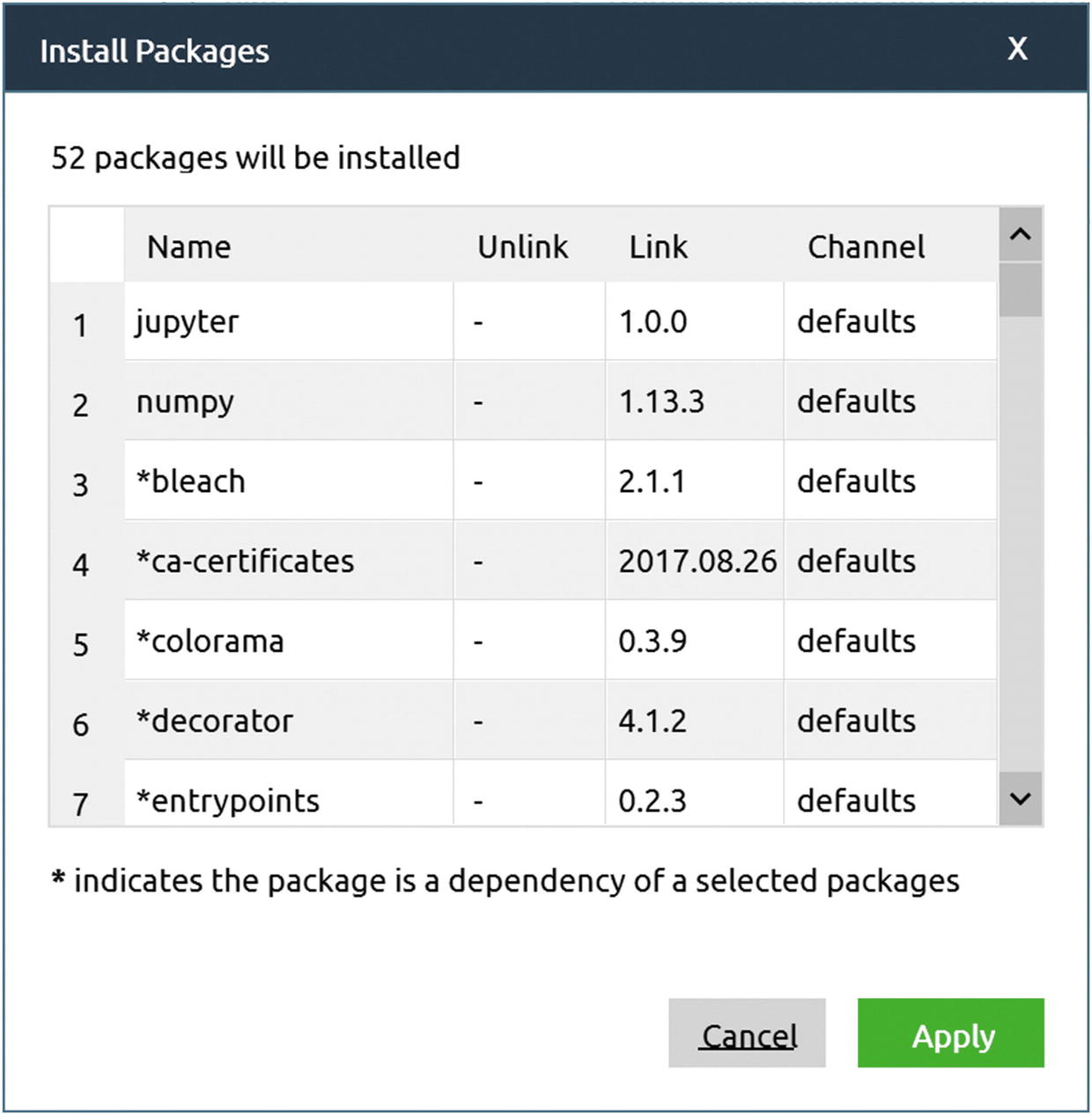
When installing a package, the Anaconda navigator will check if what you want to install depends on other packages that are not installed. In such a case, it will suggest that you install the missing (but necessary) packages from an additional window. In our case, 52 additional packages were required by the NumPy library on a newly installed system. Simply click Apply to install all of them.
numpy (1.13.3): For doing numerical calculations
matplotlib (2.1.1): To produce nice plots, as the ones you will see in this book
scikit-learn (0.19.1): This package contains all the libraries related to machine learning and that we use, for example, to load datasets.
jupyter (1.0.0): To be able to use the Jupyter notebooks
Installing TensorFlow
Installing TensorFlow is slightly more complex. The best way to do this is to follow the instructions given by the TensorFlow team, available at the following address: www.tensorflow.org/install/ .

If you type “anaconda” in the Start menu search field in Windows 10, you should see at least two entries: Anaconda Navigator, where you created the TensorFlow environment, and Anaconda Prompt
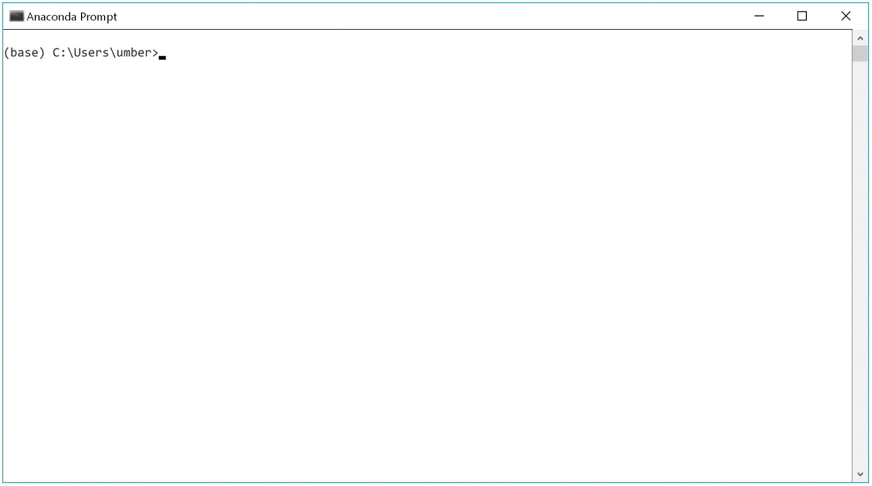
This is what you should see when you select Anaconda Prompt. Note that the user name will be different. You will see not umber (my username) but your username.
At the command prompt , you first must activate your new “tensorflow” environment. This is necessary to let the Python installation know in which environment you want to install TensorFlow. To do this, simply type the following command: activate tensorflow. Your prompt should change to this: (tensorflow) C:Usersumber>.
Remember: Your username will be different (you will see not umber in your prompt but your username). I will assume here that you will install the standard TensorFlow version that uses only the CPU (and not the GPU) version. Just type the following command: pip install --ignore-installed --upgrade tensorflow.
Now let the system install all the necessary packages. This may take a few minutes (depending on several factors, such as your computer speed or your Internet connection). You should not receive any error message. Congratulations! Now you have an environment in which you can run code using TensorFlow.
Jupyter Notebooks
The Jupyter Notebook is an open-source web application that allows you to create and share documents that contain live code, equations, visualizations and narrative text. Uses include: data cleaning and transformation, numerical simulation, statistical modeling, data visualization, machine learning, and much more.
It is widely used in the machine learning community, and it is a good idea to learn how to use it. Check the Jupyter project web site at http://jupyter.org/ .
This site is very instructive and includes many examples of what is possible. All the code you find in this book has been developed and tested using Jupyter notebooks. I assume that you already have some experience with this web-based development environment. In case you need a refresher, I suggest you check the documentation you can find on the Jupyter project web site at the following address: http://jupyter.org/documentation.html .
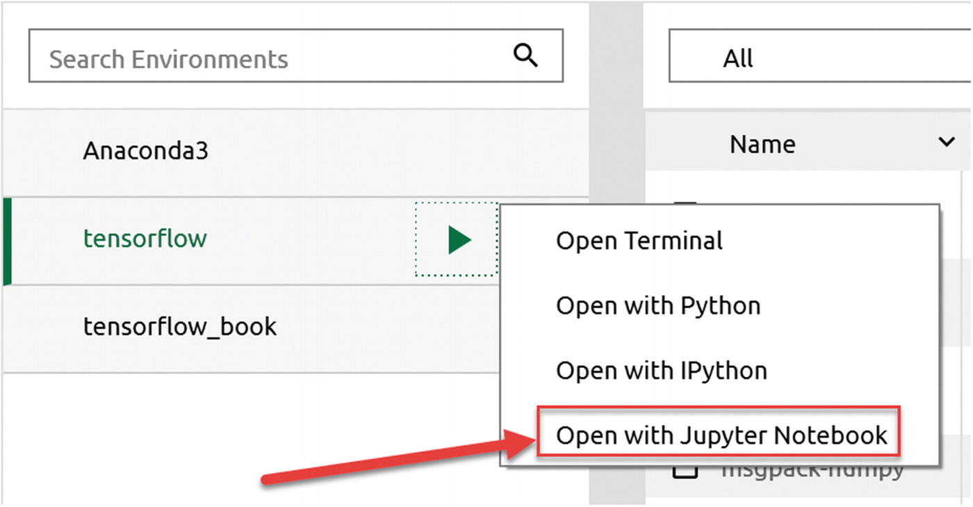
To start a Jupyter notebook in your new environment, click the triangle to the right of the “tensorflow” environment name and click Open with Jupyter Notebook
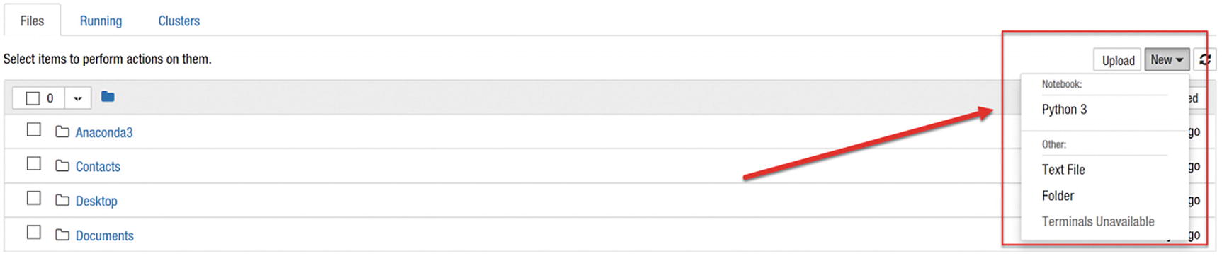
To create a new notebook, click the New button located at the top-right corner of the page and select Python 3
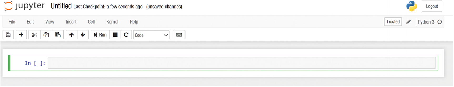
When you create an empty notebook, an empty page will open that should look like this one
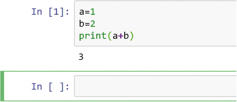
After typing some code in the cell, pressing Shift+Enter will evaluate the code in the cell
The preceding code gives the result of a+b, that is, 3. A new empty cell for you to type in is automatically created after the result is given. For more information on how to add comments, equations, inline plots, and much more, I suggest that you visit the Jupyter web site and check the documentation provided.
Note
In case you forget the folder your notebook is in, you can check the URL of the page. For example, in my case, I have http://localhost:8888/notebooks/Documents/Data%20Science/Projects/Applied%20advanced%20deep%20learning%20(book)/chapter%201/AADL%20-%20Chapter%201%20-%20Introduction.ipynb. You will notice that the URL is simply a concatenation of the folders in which the notebook is located, separated by a forward slash. A %20 character simply means a space. In this case, my notebook is in the folder: Documents/Data Science/Projects/… and so forth. I often work with several notebooks at the same time, and it is useful to know where each notebook is located in case you forget (I sometimes do).
Basic Introduction to TensorFlow
Before starting to use TensorFlow, you must understand the philosophy behind it. The library is heavily based on the concept of computational graphs, and unless you understand how those work, you cannot understand how to use the library. I will give you a quick introduction to computational graphs and show you how to implement simple calculations with TensorFlow. At the end of the next section, you should understand how the library works and how we will use it in this book.
Computational Graphs

The simplest graph that we can build, showing a simple variable
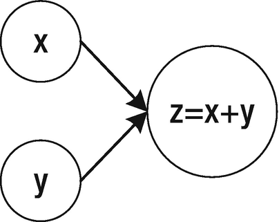
A basic computational graph for the sum of two variables
The nodes at the left of Figure 1-17 (the ones with x and y inside) are variables, while the bigger node indicates the sum of the two variables. The arrows show that the two variables, x and y, are inputs to the third node. The graph should be read (and computed) in topological order, which means that you should follow the arrows that will indicate in which order you have to compute the different nodes. The arrow will also tell you the dependencies between the nodes. To evaluate z, you first must evaluate x and y. We can also say that the node that performs the sum is dependent on the input nodes.
An important aspect to understand is that such a graph only defines the operations (in this case, the sum) to perform on two input values (in this case, x and y) to obtain a result (in this case, z). It basically defines the “how.” You must assign values to the input x and y and then perform the sum to obtain z. The graph will give you a result only when you evaluate all the nodes.
Note
In this book, I will refer to the “construction” phase of a graph, when defining what each node is doing, and the “evaluation” phase, when we will actually evaluate the related operations.
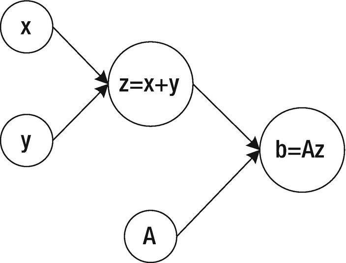
A computational graph to calculate the quantity A(x + y), given three input quantities: x, y, and A
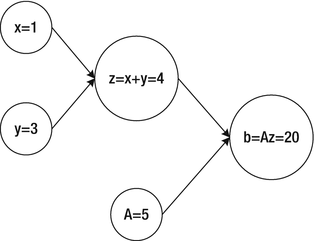
To evaluate the graph in Figure 1-18, we must assign values to the input nodes x, y, and A and then evaluate the nodes through the graph
A neural network is basically a very complicated computational graph, in which each neuron is composed by several nodes in the graph that feed its output to a certain number of other neurons, until a certain output is reached. In the next section, we will build the simplest neural network of all: one with a single neuron. Even with such a simple network, we will be able to do some pretty fun stuff.
TensorFlow allows you to build very complicated computational graphs very easily. And by construction, it separates their evaluation from the construction. (Remember that to compute a result, you must assign values and evaluate all the nodes.) In the next sections, I will show you how this works: how to build computational graphs and how to evaluate them.
Note
Remember that tensorflow first builds a computational graph (in the so-called construction phase) but does not automatically evaluate it. The library keeps the two steps separate, so that you can compute your graph several times with different inputs, for example.
Tensors
1 → a scalar
[1,2,3] → a vector
[[1,2,3], [4,5,6]] → a matrix or a two-dimensional array
Examples of Tensors with Ranks 0, 1, 2, and 3
Rank | Mathematical Entity | Python Example |
|---|---|---|
0 | Scalar (for example, length or weight) | L=30 |
1 | A vector (for example, the speed of an object in a two-dimensional plane) | S=[10.2,12.6] |
2 | A matrix | M=[[23.2, 44.2], [12.2, 55.6]] |
3 | A 3D matrix (with three dimensions) | C = [[[1],[2]],[[3],[4]], [[5], [6]]] |
data type (for example, float32)
shape (for example, [2,3], meaning a tensor with two rows and three columns)
tf.Variable
tf.constant
tf.placeholder
The tf.constant and the tf.placeholder values are, during a single-session run (more on that later), immutable. Once they have a value, they will not change. For example, a tf.placeholder could contain the dataset you want to use for training your neural network. Once assigned, it will not change during the evaluation phase. A tf.Variable could contain the weights of your neural networks. They will change during training, to find their optimal values for your specific problem. Finally, a tf.constant will never change. I will show you in the next section how to use the three different types of tensors and what aspect you should consider when developing your models.
Creating and Running a Computational Graph
Let’s start using tensorflow to create a computational graph.
Note
Remember: We always keep the construction phase (when we define what a graph should do) and its evaluation (when we perform the calculations) separate. tensorflow follows the same philosophy: first you construct a graph, and then you evaluate it.

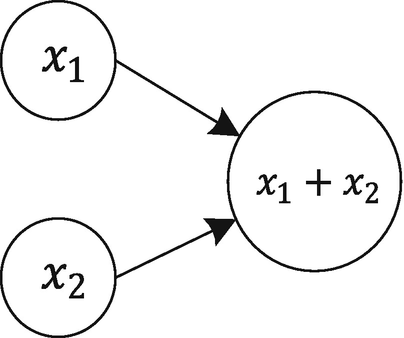
The computational graph for the sum of two tensors
Computational Graph with tf.constant
This will simply give you the evaluated result of z that is, as expected, 3. This version of the code is rather simple and does not require much, but it is not very flexible. x1 and x2 are fixed and cannot be changed during the evaluation, for example.
Note
In TensorFlow, you first must create a computational graph, then create a session, and finally run your graph. These three steps must always be followed to evaluate your graph.
Remember: You can also ask tensorflow to evaluate only an intermediate step. For example, you might want to evaluate x1 (not very interesting, but there are many cases in which it will be useful, for example, when you want to evaluate your graph and, at the same time, the accuracy and the cost function of a model), as follows: sess.run(x1).
You will get the result 1, as expected (you expected that, right?). At the end, remember to close the session with sess.close() to free up used resources.
Computational Graph with tf.Variable
This will work and give you the result 3, as you would expect.
Note
When working with variables, remember always to add a global initializer (tf.global_variables_initializer()) and run the node in your session at the beginning, before any other evaluation. We will see in many examples during the book how this works.
Computational Graph with tf.placeholder
Remember that x1=[1,5] and x2=[1,1] meaning that z=x1+x2=[1,5]+[1,1]=[2,6], because the sum is done element by element.
Use tf.placeholder for entities that will not change at each evaluation phase. Usually, those are input values or parameters that you want to keep fixed during the evaluation but may change with each run. (You will see several examples later in the book.) Examples include input dataset, learning rate, etc.
Use tf.Variable for entities that will change during the calculation, for example, the weights of our neural networks, as you will see later in the book.
Use tf.constant for entities that will never change, for example, fix values in your model that you don’t want to change anymore.
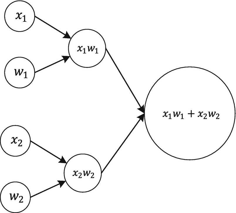
The computational graph for the calculation x1w1 + x2w2
This is simply 1 × 2 + 3 × 4 = 2 + 12 = 14 (remember that we have fed the values 1, 2, 3, and 4 in feed_dict, in the previous step). In the Chapter 2, we will draw the computational graph for a single neuron and apply what we have learned in this chapter to a very practical case. Using that graph, we will be able to do linear and logistic regression on a real dataset. As always, remember to close the session with sess.close() when you are done.
Note
In TensorFlow, it can happen that the same piece of code runs several times, and you can end up with a computational graph with multiple copies of the same node. A very common way of avoiding such a problem is to run the code tf.reset_default_graph() before the code that constructs the graph. Note that if you separate your construction code from your evaluation code appropriately, you should be able to avoid such problems. We will see later in the book in many examples how this is working.
Differences Between run and eval
And that is very useful, as will become clear in the next section about the life cycle of a node. Additionally, evaluating many nodes at the same time will make your code shorter and more readable.
will evaluate z. But this time, you must explicitly tell TensorFlow which session you want to use (you may have several defined). This is not very practical, and I prefer to use the run() method to get several results at the same time (for example, the cost function, accuracy, and F1 score). There is also a performance reason to prefer the first method, as explained in the next section.
Dependencies Between Nodes
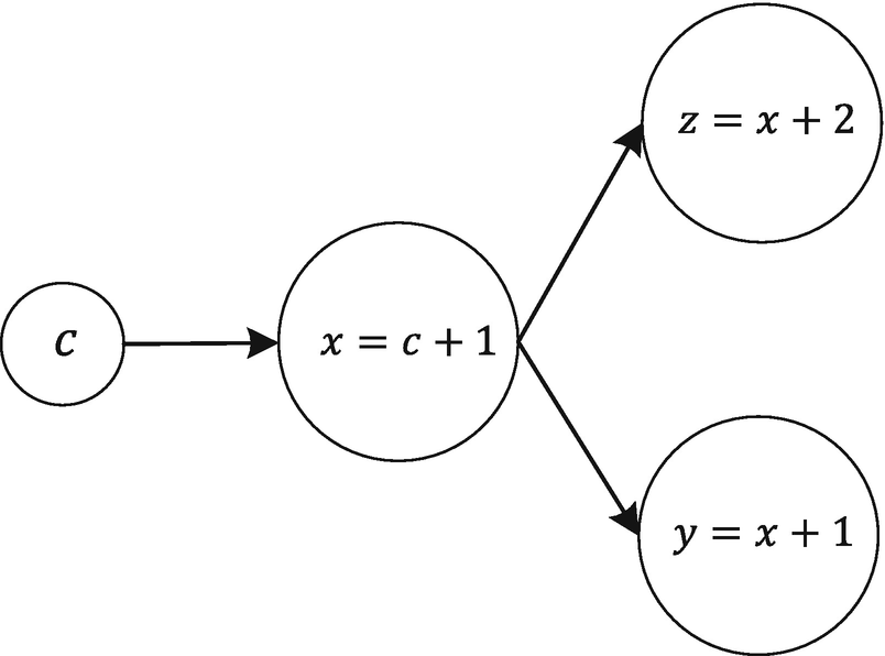
The computational graph that the code cited at the beginning of the section builds
As you can see, z and y both depend from x. The problem with the code as we have written, is that TensorFlow will not reuse the result of the previous evaluation of c and x. This means that it will evaluate the node for x one time when evaluating z and again when evaluating y. In this case, for example, using the code yy, zz = sess.run([y,z]) will evaluate y and z in one run, and x only once.
Tips on How to Create and Close a Session
There are some cases in which the explicit declaration of the session is preferred. For example, it is rather common to write a function that performs the actual graph evaluation and that returns the session, so that additional evaluation (for example, of the accuracy or similar metrics) can be done after the main training has finished. In this case, you cannot use the second version, because it would close the session immediately after finishing the evaluation, therefore making additional evaluations with the session results impossible.
Note
If you are working in an interactive environment such as Jupyter notebooks and you want to split your evaluation code on multiple notebook cells, it is easier to declare the session as sess = tf.Session(), perform the calculations needed, and then, at the end, close it. In this way, you can intercalate evaluations, graphs, and text. In case you are writing code that will not be interactive, it is sometimes preferable (and less error-prone) to use the second version, to make sure that the session is closed at the end. Additionally, with the second method, you don’t have to specify the session when using the eval() method.
The material covered in this chapter should give you all you need to build your neural networks with tensorflow. What I explained here is by no means complete or exhaustive. You should really take some time and go on the official TensorFlow web site and study the tutorials and other materials there.
Note
In this book I use a lazy programming approach. That means that I explain only what I want you to understand, nothing more. The reason is that I want you to focus on the learning goals for each chapter, and I don’t want you to be distracted by the complexity that lies behind the methods or the programming functions. Once you understand what I am trying to explain, you should invest some time and dive deeper into the methods and libraries, using the official documentation.