In this chapter, you will look at a very important technique often used when training deep networks: regularization. You will look at techniques such as the ℓ2 and ℓ1 methods, dropout, and early stopping. You will see how these methods help avoid the problem of overfitting and achieve much better results from your models, when applied correctly. You will look at the mathematics behind the methods and at how to implement it in Python and TensorFlow correctly.
Complex Networks and Overfitting
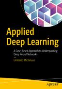
MSE for the training (continuous line) and the dev dataset (dashed line) for the neural network with 4 layers, each having 20 neurons
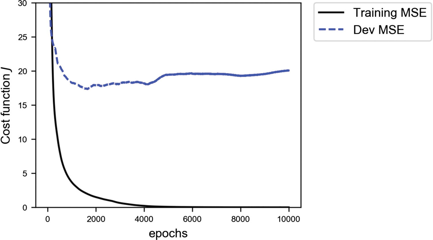
Predicted value vs. the real value for the target variable (the house price). You will notice how in the left-hand plot, for the training data, the prediction is almost perfect, while on the plot on the right, for the dev dataset, the predictions are more spread.
What can we do in this case to avoid the problem of overfitting? One solution, of course, would be to reduce the complexity of the network, that is, reducing the number of layers and/or the number of neurons in each layer. But, as you can imagine, this strategy is very time-consuming. You must try several network architectures to see how the training error and the dev error behave. In this case, this is still a viable solution, but if you are working on a problem for which the training phase takes several days, this can be quite difficult and extremely time-consuming. Several strategies have been developed to deal with this problem. The most common is called regularization, the focus of this chapter.
What Is Regularization?
Before going into the different methods, I would like to quickly discuss what the deep-learning community understands by the term regularization . The term has deeply (pun intended) evolved over time. For example, in the traditional sense (from the ’90s), the term is reserved only to as a penalty term in the loss function (Christopher M. Bishop, Neural Networks for Pattern Recognition, New York: Oxford University Press, 1995). Lately the term has gained a much more broader meaning. For example, Ian Goodfellow et al. (Deep Learning, Cambridge, MA, MIT Press, 2016) define it as “any modification we make to a learning algorithm that is intended to reduce its test error but not its training error.” Jan Kukačka et al. (“Regularization for deep learning: a taxonomy,” arXiv:1710.10686v1, available at https://goo.gl/wNkjXz ) generalize the term even further and offer the following definition: “Regularization is any supplementary technique that aims at making the model generalize better, i.e., produce better results on the test set.” So, be aware when using the term, and always be precise about what you mean.
You may also have heard or read the claim that regularization has been developed to fight overfitting. This is also a way of understanding it. Remember: A model that is overfitting the training dataset is not generalizing well to new data. This definition can also be found online, along with all the others. Although merely definitions, it is important to have a familiarity with them, so that you may better understand what is meant when reading papers or books. This is a very active research area, and to give you an idea, Kukačka et al., in their review paper referenced above, list 58 different regularization methods. Yes, 58; that is not a typo. But it is important to understand that in their general definition, SGD (stochastic gradient descent) also is considered a regularization method, something not everyone agrees on. So be warned, when reading research material, check what is understood by the term regularization.
In this chapter, you will look at the three most common and well-known methods: ℓ1, ℓ2, and dropout, and I will briefly discuss early stopping, although this method does not, technically speaking, fight overfitting. ℓ1 and ℓ2 achieve a so-called weight decay, by adding a so-called regularization term to the cost function, while dropout simply removes, in a random fashion, nodes from the network during the training phase. To understand the three methods properly, we must study them in detail. Let’s start with probably the most instructive one: ℓ2 regularization.
At the end of the chapter, we will explore a few other ideas about how to fight overfitting and get the model to generalize better. Instead of changing or modifying the model or the learning algorithm, we will consider strategies with the idea of modifying the training data, to make learning more effective.
About Network Complexity
I would like to spend a few moments discussing briefly a term I’ve used very often: network complexity. You have read here, as you can almost anywhere, that with regularization, you want to reduce network complexity. But what does that really mean? Actually, it is relatively difficult to give a definition of network complexity, so much so that no one does it. You can find several research papers on the problem of model complexity (note that I did not say network complexity), with roots in information theory. You will see in this chapter how, for example, the number of weights that is different than zero will change dramatically with the number of epochs, with the optimization algorithm, and so on, therefore making this vaguely intuitive concept of complexity dependent also on how long you train your model. To make a long story short, the term network complexity should be used only on an intuitive level, because, theoretically, it is a very complex concept to define. A complete discussion of the subject would be way beyond the scope of this book.
ℓp Norm
![$$ leftVert {x}_p
ightVert =sqrt[p]{sum limits_{kern1.5em i}{left|{x}_i
ight|}^p}kern2.125em pin mathbb{R} $$](http://images-20200215.ebookreading.net/10/2/2/9781484237908/9781484237908__applied-deep-learning__9781484237908__images__463356_1_En_5_Chapter__463356_1_En_5_Chapter_TeX_Equa.png)
where the sum is performed over all components of the vector x.
Let’s begin with the most instructive norm: the ℓ2.
ℓ2 Regularization
One of the most common regularization methods, ℓ2 regularization consists of adding a term to the cost function that has the goal of effectively reducing the capacity of the network to adapt to complex datasets. Let’s first have a look at the mathematics behind the method.
Theory of ℓ2 Regularization

 is the predicted value, w is the vector of all the weights of our network, including the bias, and m is the number of observations. Now let’s define a new cost function


is called a regularization term and is nothing else than the ℓ2-norm squared of w multiplied by a constant factor λ/2m. λ is called the regularization parameter.
Note
The new regularization parameter, λ, is a new hyperparameter that you must tune to find the optimal value.
![$$ {w}_{j,left[n+1
ight]}={w}_{j,left[n
ight]}-gamma frac{partial ilde{J}left({w}_{left[n
ight]}
ight)}{partial {w}_j}={w}_{j,left[n
ight]}-gamma frac{partial Jleft({w}_{left[n
ight]}
ight)}{partial {w}_j}-frac{gamma lambda}{m}{w}_{j,left[n
ight]} $$](http://images-20200215.ebookreading.net/10/2/2/9781484237908/9781484237908__applied-deep-learning__9781484237908__images__463356_1_En_5_Chapter__463356_1_En_5_Chapter_TeX_Eque.png)

![$$ {w}_{j,left[n+1
ight]}={w}_{j,left[n
ight]}left(1-frac{gamma lambda}{m}
ight)-lambda frac{partial Jleft({w}_{left[n
ight]}
ight)}{partial {w}_j} $$](http://images-20200215.ebookreading.net/10/2/2/9781484237908/9781484237908__applied-deep-learning__9781484237908__images__463356_1_En_5_Chapter__463356_1_En_5_Chapter_TeX_Equg.png)
This is the equation that we must use for the weights update. The difference with the one we already know from plain GD is that, now, the weight wj, [n] is multiplied with a constant  , and, therefore, this has the effect of effectively shifting the weight values during the update toward zero, making the network less complex (intuitively), thus fighting overfitting. Let’s try to see what is really happening to the weights, by applying the method to the Boston housing dataset.
tensorflow Implementation
 , then add it to the cost function. The model construction remains almost the same. We can do it with the following code:

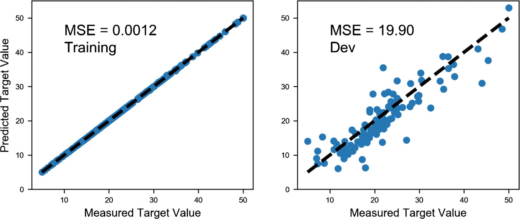
Weights distribution for each layer


Q is quite a big number. But already, without regularization, it is interesting to note that we have roughly 48% of the weights that after 10,000 epochs are less than 10−10, so, effectively, zero. This is the reason I warned you about talking about complexity in terms of numbers of learnable parameters . Additionally, using regularization will change the scenario completely. Complexity is a difficult concept to define: it depends on many things, among others, architecture, optimization algorithm, cost function, and number of epochs trained.
Note
Defining the complexity of a network only in terms of number of weights is not completely correct. The total number of weights gives an idea, but it can be quite misleading, because many may be zero after the training, effectively disappearing from the network, and making it less complex. It is more correct to talk about “Model Complexity,” instead of network complexity, because many more aspects are involved than simply how many neurons or layers the network has.
Incredibly enough, only half of the weights play a role in the predictions in the end. This is the reason I told you in Chapter 3 that defining the network complexity only with the parameter Q is misleading. Given your problem, your loss function, and optimizer, you may well end up with a network that when trained is much simpler than it was at construction phase. So be very careful when using the term complexity in the deep learning world. Be aware of the subtleties involved.
Percentage of Weights Less Than 1e-3 with and Without Regularization After 1000 Epochs
Layer | % of Weights Less Than 1e-3 for λ = 0 | % of Weights Less Than 1e-3 for λ = 3 |
|---|---|---|
1 | 0.0 | 20.0 |
2 | 0.25 | 41.5 |
3 | 0.75 | 60.5 |
4 | 0.25 | 66.0 |
5 | 0.0 | 35.0 |

Behavior of the MSE for the training (continuous line) dataset and for the dev (dashed) dataset for our network varying λ.
As you can see with small values of λ (effectively without regularization), we are in an overfitting regime (MSEtrain ≪ MSEdev): slowly the MSEtrain increases, while the MSEdev remains roughly constant. Until λ ≈ 7.5, the model overfits the training data, then the two values cross, and the overfitting finishes. After that, they grow together, at which point the model cannot capture the fine data structures anymore. After the crossing of the lines, the model becomes too simple to capture the features of the problem, and, therefore, the errors grow together, and the error on the training dataset gets bigger, because the model doesn’t even fit the training data well. In this specific case, a good value to choose for λ would be about 7.5, nearly the value when the two lines cross, because there, you are no longer in an overfitting region, as MSEtrain ≈ MSEdev. Remember: The main goal of having the regularization term is to get a model that generalizes in the best way possible when applied to new data. You can look at it in an even different way: a value of λ ≈ 7.5 gives you the minimum of MSEdev outside the overfitting region (for λ ≲ 7.5); therefore, it would be a good choice. Note that you may observe for your problems a very different behavior for your optimizing metric, so you will have to decide on a case-by-case basis what the best value for λ is that works for you.
Note
A good way to estimate the optimal value of the regularization parameter λ is to plot your optimizing metric (in this example, the MSE) for the training and dev datasets and observe how they behave for various values of λ. Then choose the value that gives the minimum of your optimizing metric on the dev dataset and, at the same time, gives you a model that no longer overfits your training data.

Decision boundary without regularization. White points are of the first class, and the black of the second.
Now let’s apply regularization to the network, exactly as we did before, and see how the decision boundary is modified. Here, we will use a regularization parameter λ = 0.1.

Decision boundary, as predicted by the network with ℓ2 regularization and with a regularization parameter λ = 0.1

Decision boundaries for a complex network with λ = 0.1 and for one with just one neuron. The two boundaries almost overlap completely.
ℓ1 Regularization
Now we will look at a regularization technique that is very similar to ℓ2 regularization. It is based on the same principle, adding a term to the cost function. This time, the mathematical form of the added term is different, but the method works very similarly to what I explained in the previous sections. Let’s again first have a look at the mathematics behind the algorithm.
Theory of ℓ1 Regularization and tensorflow Implementation

Weights distribution comparison between the model without the ℓ1 regularization term (λ = 0, light gray) and with ℓ1 regularization (λ = 3, dark gray)
once with λ = 0, and once with λ = 3.
As you can see, ℓ1 regularization has the same effect as ℓ2. It reduces the effective complexity of the network, reducing many weights to zero.
Comparison of Percentage of Weights Less Than 1e-3 with and Without Regularization
Layer | % of Weights Less Than 1e-3 for λ = 0 | % of Weights Less Than 1e-3 for λ = 3 |
|---|---|---|
1 | 0.0 | 52.7 |
2 | 0.25 | 53.8 |
3 | 0.75 | 46.3 |
4 | 0.25 | 45.3 |
5 | 0.0 | 60.0 |
Are Weights Really Going to Zero?
![$$ {w}_{12,5}^{left[3
ight]} $$](http://images-20200215.ebookreading.net/10/2/2/9781484237908/9781484237908__applied-deep-learning__9781484237908__images__463356_1_En_5_Chapter__463356_1_En_5_Chapter_TeX_IEq6.png) (from layer 3) plotted vs. the number of epochs for our artificial dataset with two features, ℓ2 regularization, γ = 10−3, λ = 0.1, after 1000 epochs. You can see how it quickly decreases to zero. The value after 1000 epochs is 2 · 10−21, so, for all purposes, zero.
(from layer 3) plotted vs. the number of epochs for our artificial dataset with two features, ℓ2 regularization, γ = 10−3, λ = 0.1, after 1000 epochs. You can see how it quickly decreases to zero. The value after 1000 epochs is 2 · 10−21, so, for all purposes, zero.
Weight ![$$ {w}_{12,5}^{left[3
ight]} $$](http://images-20200215.ebookreading.net/10/2/2/9781484237908/9781484237908__applied-deep-learning__9781484237908__images__463356_1_En_5_Chapter__463356_1_En_5_Chapter_TeX_IEq7.png) plotted vs. the epochs
for our artificial dataset with two features, ℓ2 regularization, γ = 10−3, λ = 0.1, trained for 1000 epochs
plotted vs. the epochs
for our artificial dataset with two features, ℓ2 regularization, γ = 10−3, λ = 0.1, trained for 1000 epochs
![$$ {w}_{j,left[n+1
ight]}={w}_{j,left[n
ight]}left(1-frac{gamma lambda}{m}
ight)-frac{gamma partial Jleft({w}_{left[n
ight]}
ight)}{partial {w}_j} $$](http://images-20200215.ebookreading.net/10/2/2/9781484237908/9781484237908__applied-deep-learning__9781484237908__images__463356_1_En_5_Chapter__463356_1_En_5_Chapter_TeX_Equk.png)
![$$ frac{partial Jleft({w}_{left[n
ight]}
ight)}{partial {w}_j}approx 0 $$](http://images-20200215.ebookreading.net/10/2/2/9781484237908/9781484237908__applied-deep-learning__9781484237908__images__463356_1_En_5_Chapter__463356_1_En_5_Chapter_TeX_Equl.png)
![$$ {w}_{j,left[n+1
ight]}-{w}_{j,left[n
ight]}=-{w}_{j,left[n
ight]}frac{gamma lambda}{m} $$](http://images-20200215.ebookreading.net/10/2/2/9781484237908/9781484237908__applied-deep-learning__9781484237908__images__463356_1_En_5_Chapter__463356_1_En_5_Chapter_TeX_Equm.png)


Weight ![$$ {w}_{12,5}^{left[3
ight]} $$](http://images-20200215.ebookreading.net/10/2/2/9781484237908/9781484237908__applied-deep-learning__9781484237908__images__463356_1_En_5_Chapter__463356_1_En_5_Chapter_TeX_IEq8.png) plotted vs. the epochs
for our artificial dataset with two features, ℓ2 regularization, γ = 10−3, λ = 0.1, trained for 1000 epochs (continuous line) together with a pure exponential decay (dashed line), provided for illustrative purposes
plotted vs. the epochs
for our artificial dataset with two features, ℓ2 regularization, γ = 10−3, λ = 0.1, trained for 1000 epochs (continuous line) together with a pure exponential decay (dashed line), provided for illustrative purposes
Note that when using regularization, you end up having tensors with a lot of zero elements, called sparse tensors. You can then profit from special routines that are extremely efficient with sparse tensors. This is something to keep in mind when you start moving toward more complex models, but a subject too advanced for this book and that would require too much space.
Dropout
This effectively removes all elements that have a probability less than keep_prob. Of much importance when doing predictions on a dev dataset is that no dropout be used!
Note
During training, dropout removes nodes randomly each iteration. But when doing predictions on a dev dataset, the entire network without dropout must be used. In other words, you must set keep_prob=1.
Dropout can be layer-specific. For example, for layers with many neurons, keep_prob can be small. For layers with a few neurons, one can set keep_prob = 1.0, effectively keeping all neurons in such layers.

Cost function for the training dataset for our model with two values of the keep_prob variable: 1.0 (no dropout) and 0.5. The other parameters are: γ = 0.01. The models have been trained for 5000 epochs. No mini-batch has been used. The oscillating line is the one evaluated with regularization.

MSE for the training and dev datasets with dropout (keep_prob=0.4)

MSE for the training and dev datasets without dropout (keep_prob=1.0)
In Figure 5-13, the MSEdev grows after dropping at the beginning. The model is in clear extreme overfitting regime (MSEtrain ≪ MSEdev), and it generalizes worse and worse when applied to the new data. In Figure 5-12, you can see how MSEtrain and MSEdev are of the same order of magnitude, and the MSEdev does not continue to grow. So, we have a model that is a lot better at generalizing than the one whose results are shown in Figure 5-13.
Note
When applying dropout, your metric (in this case, the MSE) will oscillate, so don’t be surprised when trying to find the best hyperparameters, if you see your optimizing metric oscillating.
Early Stopping

MSE for the training and the dev datasets without dropout (keep_prob=1.0). Early stopping consists in stopping the learning phase at the iteration when the MSEdev is minimum (indicated with a vertical line in the plot). At right, you can see a zoom of the left plot for the first 1000 epochs.
Early stopping simply consists of stopping the training at the point at which the MSEdev has its minimum (see Figure 5-14, the minimum is indicated by a vertical line in the figure). Note that this is not an ideal way to solve the overfitting problem. Your model will still most probably generalize very badly to new data. I usually prefer to use other techniques. Additionally, this is also time-consuming and a manual process that is very error-prone. You can get a good overview of the different application contexts by checking the Wikipedia page for early stopping: https://goo.gl/xnKo2s .
Additional Methods
Get more data. This is the simplest way of fighting overfitting. Unfortunately, very often in real life, this is not possible. Keep in mind that this is a complicated matter that I will discuss at length in the next chapter. If you are classifying cat pictures taken with a smartphone, you may think of getting more data from the Web. Although this may seem a perfectly good idea, you may discover that the images have varying quality, that possibly not all the images are really of cats (what about cat toys?). Also, you may find only images of young white cats, and so on. Basically, your additional observations may probably come from a very different distribution than your original data, and that will be a problem, as you will see. So, when getting additional data, consider the potential problems well before proceeding.
Augment your data. For example, if you are working with images, you can generate additional ones by rotating, stretching, shifting, etc., your images. That is a very common technique that may really be useful.
Resolving the problem of making the model generalize better on new data is one of machine learning’s biggest goals. It is a complicated problem that requires experience and tests. Lots of tests. Much research is going on that tries to solve these kinds of bugs when working on very complex problems. I will discuss additional techniques in the next chapter.