In this chapter, I will discuss what a neuron is and what its components are. I will clarify the mathematical notation we will require and cover the many activation functions that are used today in neural networks. Gradient descent optimization will be discussed in detail, and the concept of learning rate and its quirks will be introduced. To make things a bit more fun, we will then use a single neuron to perform linear and logistic regression on real datasets. I will then discuss and explain how to implement the two algorithms with tensorflow.
To keep the chapter focused and the learning efficient, I have left out a few things on purpose. For example, we will not split the dataset into training and test parts. We simply use all the data. Using the two would force us to do some proper analysis, and that would distract from the main goal of this chapter and make it way too long. Later in the book, I will conduct a proper analysis of the consequences of using several datasets and see how to do this properly, especially in the context of deep learning. This is a subject that requires its own chapter.
You can do wonderful, amazing, and fun things with deep learning. Let’s start to have fun!
The Structure of a Neuron
Deep learning is based on large and complex networks made up of a large number of simple computational units. Companies on the forefront of research are dealing with networks with 160 billion parameters [1]. To put things in perspective, this number is half that of the stars in our galaxy, or 1.5 times the number of people who ever lived. On a basic level, neural networks are a large set of differently interconnected units, each performing a specific (and usually relatively easy) computation. They recall LEGO toys, with which you can build very complex things using very simple and basic units. Neural networks are similar. Using relatively simple computational units, you can build very complex systems. We can vary the basic units, changing how they compute the result, how they are connected to each other, how they use the input values, and so on. Roughly formulated, all those aspects define what is known as the network architecture. Changing it will change how the network learns, how accurate the predictions are, and so on.
Those basic units are known, due to a biological parallel with the brain [2], as neurons. Basically, each neuron does a very simple thing: takes a certain number of inputs (real numbers) and calculates an output (also a real number). In this book, our inputs will be indicated by xi ∈ ℝ (real numbers), with i = 1, 2, …, nx, where i ∈ ℕ is an integer and nx is the number of input attributes (often called features). As an example of input features, you can imagine the age and weight of a person (so, we would have nx = 2). x1 could be the age, and x2 could be the weight. In real life, the number of features easily can be very big. In the dataset that we will use for our logistic regression example later in the chapter, we will have nx = 784.


Note
Practitioners mostly use the following nomenclature: wi refers to weights, b bias, xi input features, and f the activation function.
Owing to a biological parallel, the function f is called the neuron activation function (and sometimes transfer function), which will be discussed at length in the next sections.
- 1.
Combine linearly all inputs xi, calculating
 ;
; - 2.
Apply f to z, giving the output
 .
.
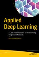
The computational graph for the neuron described in the text
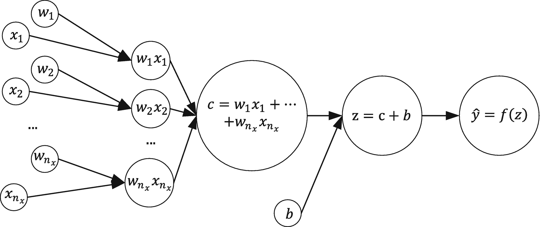
The neuron representation mostly used by practitioners
The inputs are not put in a bubble . This is simply to distinguish them from nodes that perform an actual calculation.
The weights’ names are written along the arrow. This means that before passing the inputs to the central bubble (or node), the input first will be multiplied by the relative weight, as labeled on the arrow. The first input, x1, will be multiplied by w1, x2, by w2, and so on.
The central bubble (or node) will perform several calculations at the same time. First, it will sum the inputs (the xiwi for i = 1, 2, …, nx), then sum to the result the bias b, and, finally, apply to the resulting value the activation function.


The following
representation
is a simplified version of Figure
2-2
. Unless otherwise stated, it is usually understood that the output is
 . The weights are often not explicitly reported in the neuron representation.
Matrix Notation


 as
as
 → neuron output
f(z) → activation function (or transfer function) applied to z
w → weights (vector with nx components)
b → bias
Python Implementation Tip: Loops and NumPy
The calculation that we have outlined in the equation (3) can be done in Python by standard lists and with loops, but those tend to be very slow, as the number of variables and observations grows. A good rule of thumb is to avoid loops, when possible, and to use NumPy (or TensorFlow, as we will see later) methods as often as possible.
The actual values are not relevant for our purposes. We are simply interested in how fast Python can multiply two lists, element by element. The times reported were measured on a 2017 Microsoft surface laptop and will vary greatly, depending on the hardware the code runs on. We are not interested in the absolute values, but only on how much faster NumPy is in comparison with standard Python loops. To time Python code in a Jupyter notebook, we can use a “magic command.” Usually, in a Jupyter notebook, these commands start with %% or %. A good idea is to check the official documentation, accessible from http://ipython.readthedocs.io/en/stable/interactive/magics.html , to better understand how they work.
The numpy code needed only 21 ms, or, in other words, was roughly 100 times faster than the code with standard loops. NumPy is faster for two reasons: the underlying routines are written in C, and it uses vectorized code as much as possible to speed up calculations on big amounts of data.
Note
Vectorized code refers to operations that are performed on multiple components of a vector (or a matrix) at the same time (in one statement). Passing matrices to NumPy functions is a good example of vectorized code. NumPy will perform operations on big chunks of data at the same time, obtaining a much better performance with respect to standard Python loops, which must operate on one element at a time. Note that part of the good performance NumPy is showing is also owing to the underlying routines being written in C.
While training deep learning models, you will find yourself doing this kind of operation over and over, and, therefore, such a speed gain will make the difference between having a model that can be trained and one that will never give you a result.
Activation Functions
There are many activation functions at our disposal to change the output of our neuron. Remember: An activation function is simply a mathematical function that transforms z in the output  . Let’s have a look at the most used.
Identity Function


The identity function
Sigmoid Function

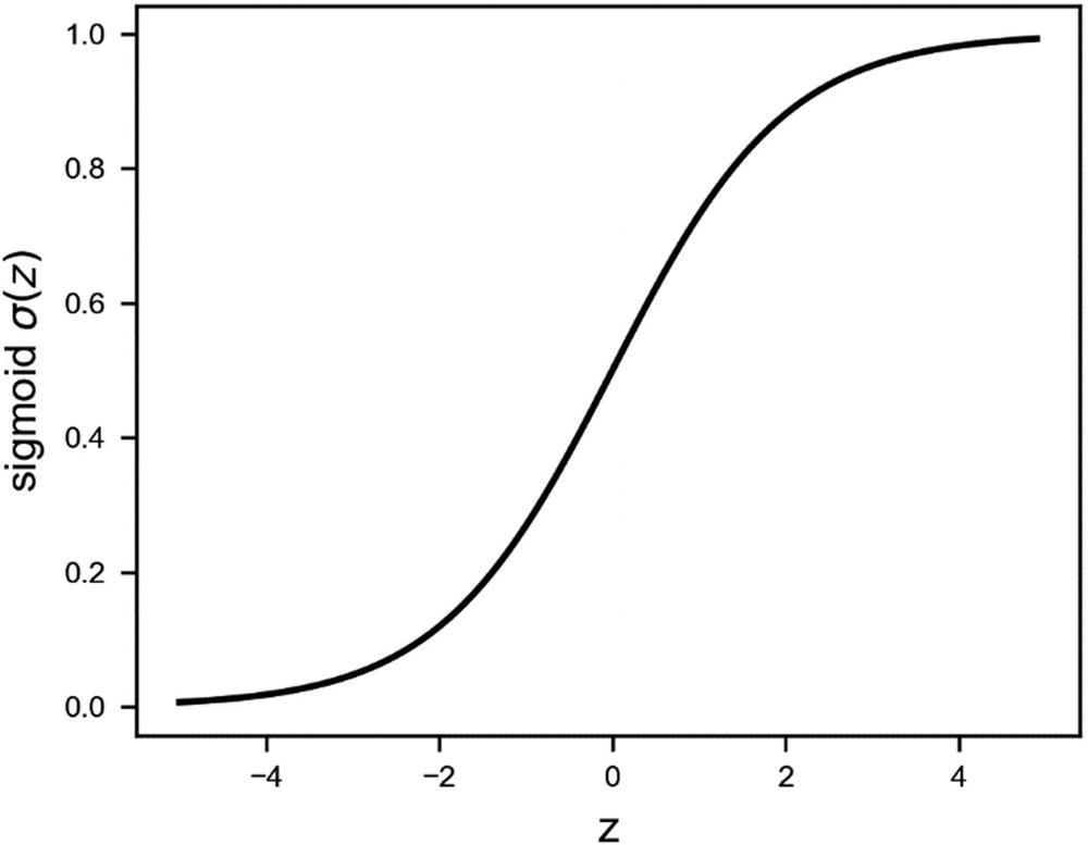
The sigmoid activation function is an s-shaped function that goes from 0 to 1
Note
Although σ(z) should never be exactly 0 or 1, while programming in Python, the reality can be quite different. due to a very big z (positive or negative), Python may round the results to exactly 0 or 1. This could give you errors while calculating the cost function (I will give you a detailed explanation and practical example later in the chapter) for classification, because we will need to calculate log σ(z) and log(1 − σ(z)) and, therefore, Python will try to calculate log0, which is not defined. This may occur, for example, if we don’t normalize our input data correctly, or if we don’t initialize our weights correctly. For the moment, it is important to remember that although mathematically everything seems under control, the reality while programming can be more difficult. It is something that is good to keep in mind while debugging models that, for example, give nan as a result for the cost function.
Note
It is very useful to know that if we have two numpy arrays, A and B, the following are equivalent: A/B is equivalent to np.divide(A,B), A+B is equivalent to np.add(A,B), A-B is equivalent to np.subtract(A,B), and A*B is equivalent to np.multiply(A,B). In case you are familiar with object-oriented programming, we say that in numpy, basic operations, such as /, *, +, and -, are overloaded. Note also that all of these four basic operations in numpy act element by element.
As stated previously, 1.0 + np.exp(-z) is equivalent to np.add(1.0, np.exp(-z)), and 1.0 / (np.add(1.0, np.exp(-z))) to np.divide(1.0, np.add(1.0, np.exp(-z))). I want to draw your attention to another point in the formula. np.exp(-z) will have the dimensions of z (usually a vector that will have a length equal to the number of observations), while 1.0 is a scalar (a one-dimensional entity). How can Python sum the two? What happens is what is called broadcasting.1 Python, subject to certain constraints, will “broadcast ” the smaller array (in this case, the 1.0) across the larger one, so that at the end, the two have the same dimensions. In this case, the 1.0 becomes an array of the same dimension as z, all filled with 1.0. This is an important concept to understand, as it is very useful. You don’t have to transform numbers in arrays, for example. Python will take care of it for you. The rules on how broadcasting works in other cases are rather complex and beyond the scope of this book. However, it is important to know that Python is doing something in the background.
Tanh (Hyperbolic Tangent Activation) Function


The tanh (or hyperbolic function) is an s-shaped curve that goes from -1 to 1
ReLU (Rectified Linear Unit) Activation Function


It is useful to spend a few moments exploring how to implement the ReLU function in a smart way in Python. Note that when we will start using TensorFlow, we will have it already implemented for us, but it is very instructive to observe how different Python implementations can make a difference when implementing complex deep-learning models.
- 1.
np.maximum(x, 0, x)
- 2.
np.maximum(x, 0)
- 3.
x * (x > 0)
- 4.
(abs(x) + x) / 2
The difference is stunning . The Method 1 is four times faster than the Method 4. The numpy library is highly optimized, with many routines written in C. But knowing how to code efficiently still makes a difference and can have a great impact. Why is np.maximum(x, 0, x) faster than np.maximum(x, 0)? The first version updates x in place, without creating a new array. This can save a lot of time, especially when arrays are big. If you don’t want to (or can’t) update the input vector in place, you can still use the np.maximum(x, 0) version.
Note
Remember: When optimizing your code, even small changes may make a huge difference. In deep-learning programs, the same chunk of code will be repeated millions and billions of times, so even a small improvement will have a huge impact in the long run. Spending time to optimize your code is a necessary step that will pay off.
Leaky ReLU

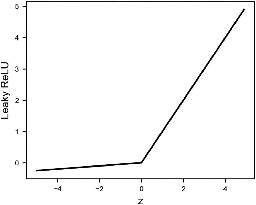
The Leaky ReLU activation function with α = 0.05
Swish Activation Function


The Swish activation function for three different values of the parameter β
ImageNet is a large database of images that is often used to benchmark new network architectures or algorithms, such as, in this case, networks with a different activation function.
Other Activation Functions
ArcTan

Exponential Linear unit (ELU)

Softplus

Note
Practitioners almost always use only two activation functions: the sigmoid and the ReLU (the ReLU probably most often). With both, you can achieve good results, and, given a complex enough network architecture, both can approximate any nonlinear function [5,6]. Remember that when using tensorflow, you will not have to implement the functions by yourself. tensorflow will offer an efficient implementation for you to use. But it is important to know how each activation function behaves, to understand when to use which one.
Cost Function and Gradient Descent : The Quirks of the Learning Rate
Now that you understand clearly what a neuron is, I will discuss what it means for it (and, in general, for a neural network) to learn. This will allow us to introduce concepts such as hyperparameters and learning rate. In almost all neural network problems, learning simply means finding the weights (remember that a neural network is composed of many neurons, and each neuron will have its own set of weights) and biases of the network that minimize a chosen function, which is usually called the cost function and typically indicated by J.
In calculus, there are several methods for finding the minimum of a given function analytically. Unfortunately, in all neural network applications, the number of weights is so big that it is not possible to use these methods. Numerical methods must be relied on, the most famous being gradient descent. It is the easiest method to understand, and it will give you the perfect basis from which to understand the more complex algorithms that you will see later in the book. Let me give a brief overview on how it works, because it is one of the best algorithms in machine learning to introduce the reader to the concept of learning rate and its quirks.
- 1.
Iteration 0: Choose a random initial guess w0
- 2.
Iteration n + 1 (with n starting from 0): The weights at iteration n + 1, wn + 1 will be updated from the previous values at iteration n, wn, using the formula


To decide when to stop, we could check when the cost function J(w) stops changing too much, or, in other words, you could define a threshold ϵ and stop at any iteration q > k (with k an integer that you have to find) that satisfies | J(wq + 1) − J(wq) | < ϵ for all q > k. The problem with this approach is that it is complicated, and this check is very expensive in terms of performance when implemented in Python (remember: you will have to do this step a very large number of times), so, usually, people simply let the algorithm run for a fixed big number of iterations and check the final results. If the result is not what is expected, they increase the fixed big number. How big? Well, that depends on your problem. What you do is choose a certain number of iterations (for example, 10,000 or 1,000,000) and let the algorithm run. At the same time, you plot the cost function vs. the number of iterations, and you check that the number of iterations you have chosen is sensible. Later in this chapter, you will see a practical example in which I will show you how to check if the number you chose was big enough. For the moment, you should know that you simply stop the algorithm after a fixed number of iterations.
Note
Why this algorithm converges toward the minimum (and how to show it) is beyond the scope of this book, would make this chapter too long, and distract the reader from the main learning goal, which is to make you understand what the effect of choosing a specific learning rate is and what the consequences are of choosing too big or too small a rate.
We will assume here that the cost function is differentiable. This is not usually the case, but a discussion of this issue goes well beyond the scope of this book. People tend to use a practical approach in this case. The implementations work very well, and so these kinds of theoretical problems are usually ignored by a large number of practitioners. Remember that in deep-learning models, the cost function becomes an incredibly complex function, and studying it is almost impossible.
The series wn will hopefully converge toward the minimum location, after a reasonable amount of iterations. The parameter γ is called the learning rate and is one of the most important parameters required in the neural network learning process.
Note
To distinguish it from weights, the learning rate is called a hyperparameter. We will encounter more of those. A hyperparameter is a parameter whose value is not determined by training and usually set before the learning process begins. In contrast, the values of parameters w and b are derived via training.
The word hopefully, has been chosen for good reason. It is possible that the algorithm will not converge toward the minimum. It is even possible that the series wn will oscillate between values without converging at all—or diverge outright. Choose γ too big or too small, and your model will not converge (or converge too slowly). To understand why this is the case, let’s consider a practical case and see how the method works while choosing different learning rates.
Learning Rate in a Practical Example

 the jth feature and the ith observation. In the example here, we have just one feature, so we don’t need the subscript j. The cost function can be implemented in Python easily as
Our goal is to find the values for w0 and w1 that minimize J(w0, w1).


Because ∂f(w0, w1, xi)/∂w0 = 1 and ∂f(w0, w1, xi)/∂w1 = xi, the previous equations are the ones that must be implemented in Python, if we want to code the gradient descent algorithm by ourselves.
Note
The derivation of the equations in (2.11) has the goal of showing how the equations for gradient descent become very complicated very quickly, even for a very easy case. In the next section, we will build our first model with tensorflow. One of the best aspects of the library is that all those formulas are calculated automatically, and you don’t have to bother calculating anything. Implementing equations such as the ones in shown here and debugging them can take quite some time and prove to be impossible the moment you are dealing with large neural networks of interconnected neurons.
I have omitted in this book the complete Python implementation of the example, because it would require too much space.
It is instructive to check how the model works, by varying the learning rate. In Figures 2-10, 2-11, and 2-12, the contour lines2 of the cost functions have been drawn, and on top of these, the series (w0, n, w1, n) has been plotted, as points to visualize how the series converges (or doesn’t). In the figures, the minimum is indicated by a circle placed approximately at the center. We will consider the values γ = 0.8 (in Figure 2-10), γ = 2 (in Figure 2-11), and γ = 0.05 (in Figure 2-12). The different estimates, wn, are indicated with points. The minimum is indicated by the circle approximately in the middle of the image.
In the first case (in Figure 2-10), the converging is well behaved, and in just eight steps, the method converges toward the minimum. When γ = 2 (Figure 2-11), the method makes steps that are too big (remember: the steps are given by −γ∇J(w) and therefore the bigger γ the bigger the steps) and unable to get close to the minimum. It keeps oscillating around it, without reaching it. In this case, the model will never converge. In the last case, when γ = 0.05 (Figure 2-12), the learning is so slow that it will take many more steps to get close to the minimum. In some cases, the cost function may be so flat around the minimum that the method takes such a big number of iterations to converge that, practically, you will not get close enough to the real minimum in a reasonable amount of time. In Figure 2-12, 300 iterations are plotted, but the method is not even very close to the minimum.
Note
Choosing the right learning rate is of paramount importance when coding the learning part of a neural network. Choose too big a rate, and the method may just bounce around the minimum, without ever reaching it. Choose too small a rate, and the algorithm may become so slow that you will not be able to find the minimum in a reasonable amount of time (or number of iterations). A typical sign of a learning rate that is too big is that the cost function may become nan (“not a number,” in Python slang). Printing the cost function at regular intervals during the training process is a good way of checking such kind of problems. This will give you a chance to stop the process and avoid wasting time (in case you see nan appearing). A concrete example appears later in the chapter.

Illustration of a gradient descent algorithm with well-behaved convergence
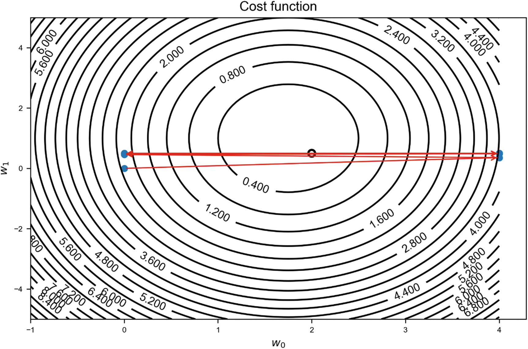
Illustration of a gradient descent algorithm when the learning rate is too big. The method is not able to converge toward the minimum.
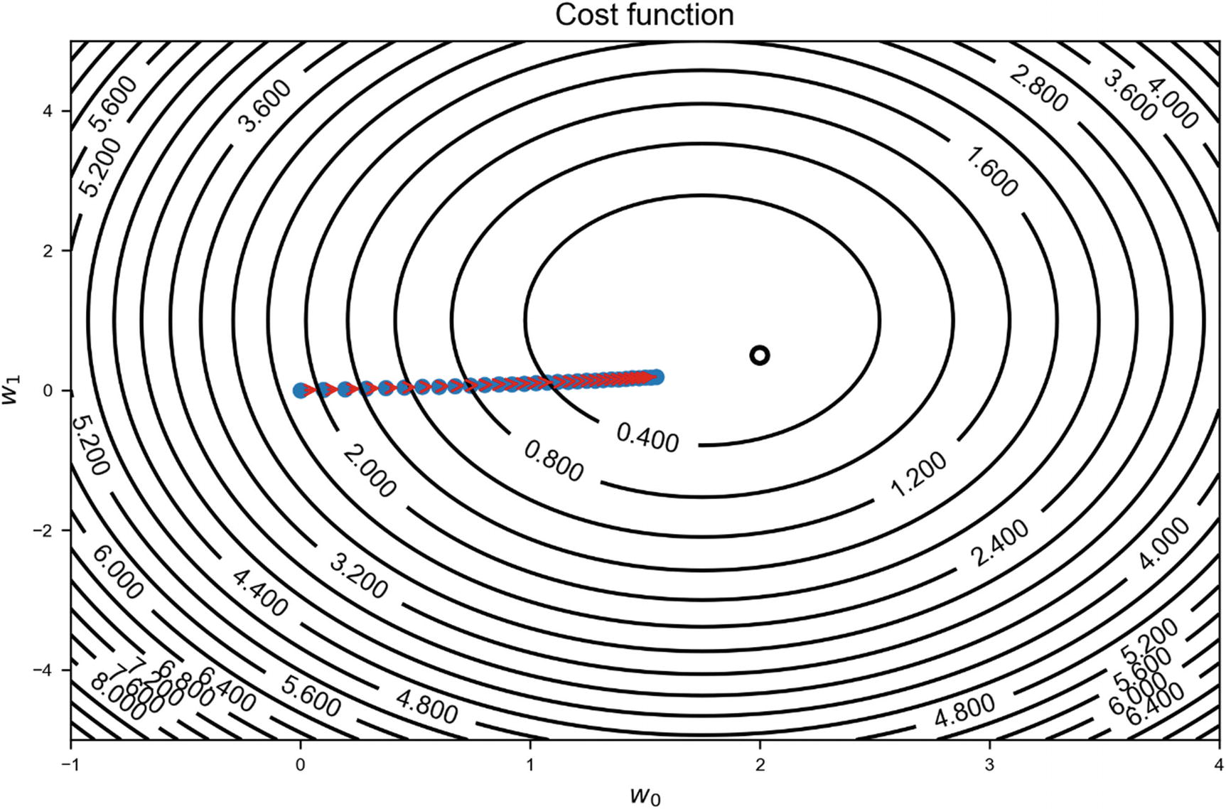
Illustration of a gradient descent algorithm when the learning rate is too small. The method is so slow that it will take a huge number of iterations to converge toward the minimum.
Sometimes it is efficient to change the learning rate during the process. You start with a bigger value to get close to the minimum faster, and then you reduce it progressively, to make sure that you get as close as possible to the real minimum. I will discuss this approach later in the book.
Note
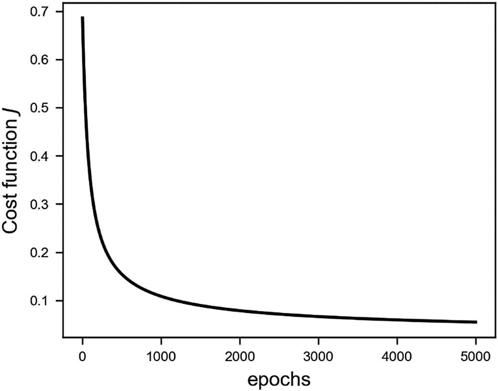
There are no fixed rules on how to choose the right learning rate. It depends on the model, on the cost function, on the starting point, and so on. A good rule of thumb is to start with γ = 0.05 and then see how the cost function behaves. It is rather common to plot J(w) vs. the number of iterations, to check that it decreases and the speed at which it is decreasing.

The cost function vs. the number of iterations (only the first eight are considered)
γ = 0.05 → J is decreasing, which is good, but after eight iterations, we have not reached a plateau, so we must use many more iterations, until we see that J is not changing much anymore.
γ = 2 → J is not decreasing. We should check our learning rate to see if it helps. Trying smaller values would be a good starting point.
γ = 0.8 → The cost function decreases rather quickly and then remains constant. That is a good sign and indicates that we have reached a minimum.
Remember also that the absolute value of the learning rate is not relevant. What is important is the behavior. We can multiply our cost function by a constant, and that would not influence our learning at all. Don’t look at the absolute values; check how fast and how the cost function is behaving. Additionally, the cost function will almost never reach zero, so don’t expect it. The value of J at its minimum is almost never zero (it depends on the functions itself). In the section about linear regression, you will see an example in which the cost function will not reach zero.
Note
When training your models, remember to always check the cost function vs. the number of iterations (or number of swipes over the entire training set, called epochs). This will give you an efficient way of estimating if the training is efficient, if it is working at all, and give you hints on how to optimize it.
Now that we have defined the basis, we will use a neuron to solve two simple problems with machine learning: linear and logistic regression.
Example of Linear Regression in tensorflow
The first type of regression will offer an opportunity to understand how to build a model in tensorflow. To explain how to perform linear regression efficiently with one neuron, I must first explain some additional notation. In the previous sections, I discussed inputs  . These are the so-called features that describe an observation. Normally, we have many observations. As briefly explained before, we will use an upper index to indicate the different observations between parentheses. Our ith observation will be indicated with x(i), and the jth feature of the ith observations will be indicated as
  . We will indicate the number of observations with m.
Note
In this book, m is the number of observations, and nx is the number of features. Our jth feature of the ith observation will be indicated with  . In deep-learning projects, the bigger the m the better. So be prepared to deal with a huge number of observations.
You will remember that I have said many times that numpy is highly optimized to perform several parallel operations at the same time. To get the best performance possible, it is important to write our equations in matrix form and feed the matrices to numpy. In this way, our code will be as efficient as possible. Remember: Avoid loops at all costs whenever possible. Let’s spend some time now in writing all our equations in matrix form. In this way, our Python implementation will be much easier later.

 in matrix form. If you recall our neuron discussion, we have defined a z(i) = wTx(i) + b for one observation i. Putting each observation in a column, we can use the following notation:
 as
as
where with f (z), we intend the function f be applied element by element to the matrix z.
Note
Although z has dimensions 1 × m, we will use the term matrix for it and not vector, to use consistent names in the book. This will also help you to remember that we should always use matrix operations. For our purposes, z is simply a matrix with just one row.
X has dimensions nx × m
z has dimensions 1 × m
 has dimensions 1 × m
w has dimensions nx × 1
b has dimensions 1 × m
Now that the formalism is clear, we will prepare the dataset.
Dataset for Our Linear Regression Model
CRIM: Per capita crime rate by town
ZN: Proportion of residential land zoned for lots over 25,000 square feet
INDUS: Proportion of non-retail business acres per town
CHAS: Charles River dummy variable (= 1 if tract bounds river; 0 otherwise)
NOX: Nitric oxides concentration (parts per 10 million)
RM: Average number of rooms per dwelling
AGE: Proportion of owner-occupied units built prior to 1940
DIS: Weighted distances to five Boston employment centers
RAD: Index of accessibility to radial highways
TAX: Full-value property-tax rate per $10,000
PTRATIO: Pupil-teacher ratio by town
B - 1000(Bk - 0.63)^2 - Bk: Proportion of blacks by town
LSTAT: % lower status of the population
MEDV: Median value of owner-occupied homes in $1000s
Our target variable MEDV, the one we want to predict, is the median price of the house in $1000s for each suburb. For our example, we don’t have to understand or study the features . My goal here is to show you how to build a linear regression model with what you have learned. Normally, in a machine-learning project, you would first study your input data, check their distribution, quality, missing values, and so on; however, I will skip this part to concentrate on how to implement what you learned with tensorflow.
Note
In machine learning, the variable we want to predict is usually called the target variable.
 according to the formula
 is the average
of the jth feature, and
is the average
of the jth feature, and  is its standard deviation. This can be easily calculated in numpy with the following function:
To normalize our features numpy array, we must simply call the function features_norm = normalize(features). Now each feature contained in the numpy array features_norm will have an average of zero and a standard deviation of one.
Note
It is generally a good idea to normalize the features, so that their average is zero, and the standard deviation is one. Sometimes, some features are much bigger than others and can have a stronger influence on the model, thus bringing wrong predictions. Particular care is needed when the dataset is split into training and test datasets, to have consistent normalizations.
The train_x array has dimensions of (13, 506), and that is exactly what we expect. Remember for our discussion that X has dimensions nx × m.
Neuron and Cost Function for Linear Regression

where the sum is over all m observations.
Note that in tensorflow, you don’t have to explicitly declare the number of observations. You can use None in the code. In this way, you will be able to run the model on any dataset independently of the number of observations, without modifying your code.
 as y_, because we don’t have a hat in Python. Let me clarify a bit which line of code does what.
X = tf.placeholder(tf.float32, [n_dim, None]) → contains the matrix X, which must have dimensions nx × m. Remember that in our code, n_dim is nx and that m is not declared explicitly in tensorflow. In its place, we use None.
Y = tf.placeholder(tf.float32, [1, None]) → contains the output values
 , which must have dimensions 1 × m. Here, this means that instead of m, we use None, because we want to use the same model for different datasets (that will have a different number of observations).
learning_rate = tf.placeholder(tf.float32, shape=()) → contains the learning rate as a parameter instead of a constant, so that we can run the same model varying it, without creating a new neuron each time.
W = tf.Variable(tf.zeros([n_dim, 1])) → defines and initializes the weights, w, with zeros. Remember that the weights, w, must have dimensions nx × 1.
b = tf.Variable(tf.zeros(1)) → defines and initializes the bias, b, with zero.
init = tf.global_variables_initializer() → creates a piece of the graph that initializes the variable and adds it to the graph.
y_ = tf.matmul(tf.transpose(W),X)+b → calculates the output of the neuron. The output of a neuron is
 . Because the activation function for linear regression is the identity, the output is
  . Remember that b being a scalar is not a problem. Python broadcasting will take care of it, expanding it to the right dimensions
, to make the sum between a vector wT X and a scalar b possible.
. Remember that b being a scalar is not a problem. Python broadcasting will take care of it, expanding it to the right dimensions
, to make the sum between a vector wT X and a scalar b possible.cost = tf.reduce_mean(tf.square(y_-Y)) → defines the cost function. tensorflow provides an easy and efficient way of calculating the average—tf.reduce_mean()—that simply performs the sum of all the elements of the tensor and divides it by the number of elements.
training_step = tf.train.GradientDescentOptimizer(learning_rate).minimize(cost) → tells tensorflow which algorithm to use to minimize the cost function. In tensorflow language, the algorithms used to minimize the cost function are called optimizers. We now use gradient descent with the given learning rate. Later in the book, other optimizers will be extensively studied.
sess = tf.Session() → creates a tensorflow session.
sess.run(init) → runs the initialization of the different element of the graphs.
cost_history = np.empty(shape=[0], dtype = float) → creates an empty vector (for the moment with zero elements) in which the value of our cost function at each iteration is stored.
for loop... → In this loop, tensorflow performs the gradient descent steps that we have discussed earlier and updates the weights and the bias. In addition, it will save in the array cost_history the value of the cost function each time: cost_history = np.append(cost_history, cost_).
if (epoch % 1000 == 0)... → Every 1000 epochs we will print the value of the cost function. This is an easy way of checking if the cost function is really decreasing or if nans are appearing. If you perform some initial tests in an interactive environment (such as a Jupyter notebook), you can stop the process if you see that the cost function is not behaving as you expect.
return sess, cost_history → returns the session (in case you want to calculate something else) and the array containing the cost function values (we will use this array to plot it).

The cost function resulting in our model applied to the Boston dataset with a learning rate of γ=0.01. We plot only the first 500 epochs, since the cost function has almost already reached its final value.

The predicted target value vs. the measured target value for our model, applied to our trianing data
The points lay reasonably well around the line, so it seems we can predict our price to a certain degree. A more qualitative method for estimating the accuracy of our regression is the MSE itself (which, in our case, is simply our cost function). Whether the value we are obtaining (22.08 in 1000 USD) is good enough depends on the problem you are trying to solve, or the constraint and requirements you have been given.
Satisficing and Optimizing a Metric
We have seen that it is not easy to decide whether a model is good. Figure 2-15 will not allow us to describe quantitively how good (or not good) our model is. For this, we must define a metric.
Satisficing metric → Searching through available alternatives until an acceptability threshold is met, for example, code running (RT) time, which minimizes the cost function subject to RT < 1 sec, or choosing among modes the one that has an RT < 1 sec
Optimizing metric → Searching through available alternatives to maximize a specific metric, for example, choosing the model (or the hyperparameters) that maximize accuracy
Note
If you have several metrics, you should always choose one optimizing and the rest satisficing.

The cost function for linear regression applied to the Boston dataset for three learning rates: 0.1 (solid line), 0.01 (dashed line), and 0.001 (dotted line). The smaller the learning rate, the slower the learning process.
As expected for very small learning rates (0.001), the gradient descent algorithm is very slow in finding the minimum, whereas with a bigger value (0.1), the method works quickly. This kind of plot is very useful for giving you an idea of how fast and how good the learning process is going. You will see cases later in the book where the cost function is much less well behaved. For example, when applying dropout regularization, the cost function will not be smooth anymore.
Example of Logistic Regression
Logistic regression is a classic classification algorithm. To keep it simple, we will consider here a binary classification. This means that we will deal with the problem of recognizing two classes, which we will label as 0 or 1, only. We will need an activation function different from the one we used for linear regression, a different cost function to minimize, and a slight modification of the output of our neuron. Our goal is to be able to build a model that can predict if a certain new observation is of one of two classes. The neuron should give as output the probability P(y = 1| x) of the input x to be of class 1. We will then classify our observation as of class 1, if P(y = 1| x) > 0.5, or of class 0, if P(y = 1| x) < 0.5.
Cost Function


In Chapter 10, I will provide a complete derivation of logistic regression from scratch, but for the moment, tensorflow will take care of all the details—derivatives, gradient descent implementation, and so on. We only have to build the right neuron, and we will be on our way.
Activation Function

The Dataset
To build an interesting model, we will use a modified version of the MNIST dataset. You will find all relevant information from the following link: http://yann.lecun.com/exdb/mnist/ .
The MNIST database is a large database of handwritten digits that we can use to train our model. The MNIST database contains 70,000 images. “The original black and white (bilevel) images from NIST were size normalized to fit in a 20×20 pixel box while preserving their aspect ratio. The resulting images contain grey levels as a result of the anti-aliasing technique used by the normalization algorithm. The images were centered in a 28×28 image by computing the center of mass of the pixels, and translating the image so as to position this point at the center of the 28×28 field” (source: http://yann.lecun.com/exdb/mnist/ ).

The 36,003rd digit in the dataset. It is easly recognizable as a 5
Now comes a very important point. The labels in our dataset as imported will be 1 or 2 (they simply tell you which digit the image represents). However, we will build our cost function with the assumptions that our class’s labels are 0 and 1, so we must rescale our y_train_tr array.
Note
When doing binary classification, remember to check the values of the labels you are using for training. Sometimes, using the wrong labels (not 0 and 1) may cost you quite some time in understanding why the model is not working.

Six random digits chosen from the dataset. The relative rescaled labels (remember: labels in our dataset are now 0 or 1) are given in brackets.
tensorflow Implementation
 may get very close to zero or one (the sigmoid function assumes values very close to 0 or 1 for very big negative or positive values of z). Remember that in the cost function
, you have the two terms tf.log(y_) and tf.log(1-y_), and because the log function is not defined for a value of zero, if y_ is 0 or 1, you will get a nan, because the code will try to evaluate tf.log(0). As an example, we can run the model with a learning rate of 2.0. After only one epoch, you already will get a nan value for the cost function. And it is easy to understand why, if you print out the value for b before and after the first training step. Simply modify your model code and use the following version:
may get very close to zero or one (the sigmoid function assumes values very close to 0 or 1 for very big negative or positive values of z). Remember that in the cost function
, you have the two terms tf.log(y_) and tf.log(1-y_), and because the log function is not defined for a value of zero, if y_ is 0 or 1, you will get a nan, because the code will try to evaluate tf.log(0). As an example, we can run the model with a learning rate of 2.0. After only one epoch, you already will get a nan value for the cost function. And it is easy to understand why, if you print out the value for b before and after the first training step. Simply modify your model code and use the following version:You see how b goes from 0 to -0.05966223 and then to nan? Therefore, z = wTX + b turns into nan, then y = σ(z) also turns into nan, and, finally, the cost function, being a function of y, will also result in nan. This is simply because the learning rate is way too big.
What is the solution? You should try a different (read: much smaller) learning rate.

The cost function vs. epochs for a learning rate of 0.005
You could also try to run the previous model (with a learning rate of 0.005) for more epochs . You will discover that at about 7000 epochs, the nan will reappear. The solution here would be to reduce the learning rate with an increasing number of epochs. A simple approach, such as halving the learning rate every 500 epochs, will get rid of the nans. I will discuss a similar approach in more detail later in the book.
References
- [1]
Jeremy Hsu, “Biggest Neural Network Ever Pushes AI Deep Learning,” https://spectrum.ieee.org/tech-talk/computing/software/biggest-neural-network-ever-pushes-ai-deep-learning , 2015.
- [2]
Raúl Rojas, Neural Networks: A Systematic Introduction, Berlin: Springer-Verlag, 1996.
- [3]
Delve (Data for Evaluating Learning in Valid Experiments), “The Boston Housing Dataset,” www.cs.toronto.edu/~delve/data/boston/bostonDetail.html , 1996.
- [4]
Prajit Ramachandran, Barret Zoph, Quoc V. Le, “Searching for Activation Functions,” arXiv:1710.05941 [cs.NE], 2017.
- [5]
Guido F. Montufar, Razvan Pascanu, Kyunghyun Cho, and Yoshua Bengio, “On the Number of Linear Regions of Deep Neural Networks,” https://papers.nips.cc/paper/5422-on-the-number-of-linear-regions-of-deep-neural-networks.pdf , 2014.
- [6]
Brendan Fortuner, “Can Neural Networks Solve Any Problem?”, https://towardsdatascience.com/can-neural-networks-really-learn-any-function-65e106617fc6 , 2017.