Building complex networks with TensorFlow is quite easy, as you have probably realized by now. A few lines of code are enough to construct networks with thousands (and even more) parameters. It should be clear by now that problems arise while training such networks. It is difficult, unstable, and slow to test hyperparameters, because a run over a few hundred epochs may take hours. This is not only a performance problem; otherwise, it would suffice to use faster and faster hardware. The problem is that very often, the convergence process (the learning) does not work at all. It stops, it diverges, or it never gets close to the minimum of the cost function. We need ways of making the training process efficient, fast, and reliable. You will look at two of the main strategies that will help with the training of complex networks: dynamic learning rate decay and optimizers that are smarter than plain gradient descent ([GD] such as RMSProp, Momentum, and Adam).
Dynamic Learning Rate Decay
I mentioned several times that the learning rate γ is a very important parameter and that choosing it badly will make your model not perform. Refer again to Figure 2-12, which shows you how choosing a learning rate that is too big will make your gradient descent algorithm bounce around the minimum and not converge. Without discussing them, let’s rewrite the equations that describe the weight and bias update described in Chapter 2 when discussing the gradient descent algorithm. (Remember: I described the algorithm for a problem with two weights w0 and w1.)
As a reminder, following is an overview of the notation. (Please refer again to Chapter 2, if you don’t remember how the gradient descent is working.)
w0, [n]: Weight 0 at iteration n
w1, [n]: Weight 1 at iteration n
J(w0, [n], w1, [n]): Cost function at iteration n
γ: Learning rate
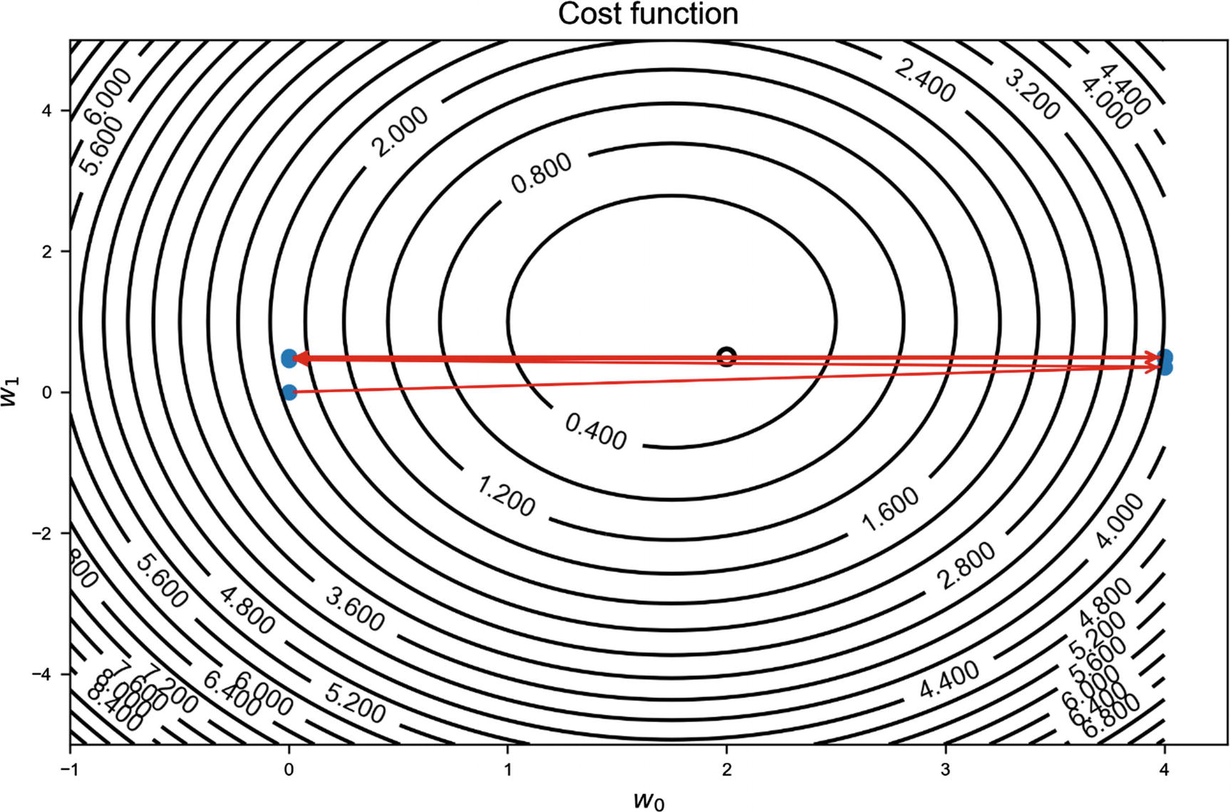
To show the effect of what I will discuss, we will consider the same problem described in the section “Learning Rate in a Practical Example,” in Chapter 2. Plotting the weights w0, n, w1, n on the contour lines of the cost function for γ = 2 (see Figure 4-1) shows (as you will remember from Chapter 2) how the values of weights oscillate around the minimum of (w0, n, w1, n). Here, the problem of a learning rate that is too big is clearly visible. The algorithm cannot converge, because the steps that it takes are too big to be able to get close to the minimum. The different estimates wn are indicated with points in Figure 4-1. The minimum is indicated by the circle approximately in the middle of the image.
Figure 4-1
Illustration of the gradient descent algorithm. Here, the learning rate of γ = 2 has been chosen
But you may have noticed that in our algorithm, we made a pretty important decision (without stating it explicitly): we keep the learning rate constant for each iteration. But there is no reason for doing so. On the contrary, it is quite a bad idea. Intuitively, a big learning rate will make the convergence move fast at the beginning, but as soon as you are around the minimum, you will want to use a much smaller learning rate, to allow the algorithm to converge in the most efficient way toward the minimum. We want to have a learning rate that starts (relatively) big and then decreases with the iterations. But how should it decrease? There are several methods that are used today, and in the next section, we will look at those used most frequently and how to implement them in Python and TensorFlow. We will use the same problem with which Figure 4-1 and 2-12 were generated and compare the behavior of the different algorithms. Please take some time to review the section in Chapter 2 on gradient descent, to have the material clear in your head before reading the next sections.
Iterations or Epochs?
Before looking at the various methods, I would like to shed some light on the question: what are the iterations we are talking about? Are they epochs? Technically, this is not the case. An iteration is when you update your weights. Consider, for example, mini-batch gradient descent. In that case, an iteration occurs after each mini-batch (when you update the weights). Consider the Zalando dataset in Chapter 3: 60,000 training cases and a mini-batch size of 50. In that case, you would have 1200 iterations in an epoch. What is important for the decrease of the learning rate is the number of updates you perform on the weights, not the number of epochs. If you used stochastic gradient descent (SGD) on the Zalando dataset (update the weights after each observation), you would have 60,000 iterations, and you might need to decrease the learning more than with mini-batch gradient descent, because it is updated more often. In the case of batch gradient descent, where you update your weight after one complete sweep over the training data, you would update the learning rate exactly once each epoch.
Note
Iterations in dynamic learning rate decay refer to the step in the algorithm in which the weights are updated. For example, if you use SGD on the Zalando dataset in Chapter 3, with a mini-batch size of 50, in one epoch (a sweep over the 60,000 training observations), you have 1200 iterations.
This is very important to understand correctly. If you do, you can choose the parameters of the different algorithms for learning rate decay properly. If you choose them thinking that the learning rate is updated only after each epoch, you may make big mistakes.
Note
For each algorithm that decreases dynamically, the learning rate will introduce new hyperparameters that you must optimize, adding some complexity to your model-selection process.
Staircase Decay
The staircase decay method is the most basic one to use. It consists of reducing the learning rate manually in the code and hard-coding the changes, based on what seems to work. For example, how can we make the GD algorithm converge in Figure 4-1, starting with a γ = 2? Let’s consider the following decay (in which we have indicated with j the iteration number):
Simply including this with the Python code
gamma0 = 2.0
if (j < 4):
gamma = gamma0
elif j>=4:
gamma = gamma0 /5.0
will give a converging algorithm (see Figure 4-2). Here, the initial learning rate of γ0 = 2 has been chosen, and from the iteration 4, γ = 0.4 has been used. The different estimates wn are indicated with points. The minimum is indicated by the circle approximately in the middle of the image. The algorithm is now able to converge. Each point has been labeled with the iteration number, to make following the weights update easier.
Figure 4-2
Illustration of gradient descent algorithm with a staircase decay method
The first steps are big, and then, as we decrease the learning rate to 0.4 at iteration 4, they become smaller, and the GD is able to converge toward the minimum. With this simple modification, we have achieved a nice result. The problem is that when dealing with complicated datasets and models (such as we did in Chapter 3), this process requires (if it works) a lot of tests. You will have to reduce the learning rate several times, and finding the right iteration and values for the learning rate decrease is a really challenging task, so much so that it is actually not usable, unless you are dealing with very easy datasets and networks. The method is also not very stable, and, depending on the data you have, may require continuous tuning. TL;DR1: don’t use it.
Table 4-1
Additional Hyperparameters Introduced
Hyperparameter
Example
The iteration at which the algorithm will update the learning rate
In this example, we choose iteration number 4
The values of the learning rate after each change (multiple values)
In this example, we had, from iteration 1 to 3, γ = 2, and, from iteration 4, γ = 0.4.
Step Decay
Something slightly more automatic is the so-called step decay. This method reduces the learning rate by a constant factor every certain number of iterations. Mathematically, it can be written as
where ⌊a⌋ indicates the integer part of a, and D (indicated in the code later with epoch_drop) is an integer constant that we can tune. For example, using the following code:
epochs_drop = 2
gamma = gamma0 / (np.floor(j/epochs_drop)+1)
will again give a convergent algorithm. In Figure 4-3, the initial learning rate of γ0 = 2 has been chosen, and every 2 iterations, the learning rate decreases according to γ0/⌊j/2+1⌋. The different estimates wn are indicated with points. The minimum is indicated by the circle approximately in the middle of the image. The algorithm is now able to converge. Each point has been labeled with the iteration number, to make following the weights update easier.
Figure 4-3
Illustration of gradient descent algorithm with step decay
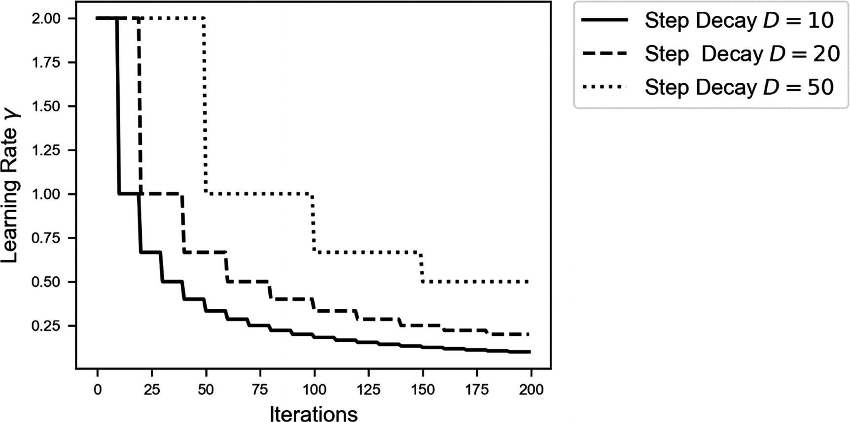
It is important to have an idea of how fast the learning rate is decreasing. You don’t want to have a learning rate close to zero after only a few iterations; otherwise, your convergence will never succeed. In Figure 4-4, you can see a comparison of how fast (or slow) the learning rate is decreasing for three values for D.
Figure 4-4
Decrease in the learning rate for three values of D: 10, 20, and 50, using the step decay algorithm
Note, for example, how with D = 10, the learning rate is roughly 10 times smaller after only 100 iterations! If you make your learning rate decrease too fast, you may see your convergence grind to a halt after only a few iterations. Always try to get an idea of how fast your γ is decreasing.
Note
A good way of getting a feel for how fast your learning rate is decreasing is to try to determine after how many iterations γ is ten times smaller than the initial value. Keep in mind that if you get a γ = γ0/10 after 10D iterations, you will get γ = γ0/100 after only 100D iterations, and γ = γ0/103 after only 103D iterations, and so on. If this occurs, what is needed can be answered only by testing the rate properly with several values of D.
Let’s consider a concrete example. Suppose you are training your model with 1e-5 observations for 5000 epochs, with a mini-batch sizes of 50 and a starting learning rate of γ0 = 0.2. If you choose D = 10 without thinking, you will have
after only 100 epochs, so you will not gain much by using 5000 epochs if you reduce the learning rate so quickly.
Table 4-2
Additional Hyperparameters Introduced
Hyperparameter
Example
Parameter D
D = 10
Inverse Time Decay
Another way of updating the learning rate is with the formula called inverse time decay
where ν is a parameter called the decay rate. In Figure 4-5, you can see a comparison of the learning rate decrease for three parameters of ν: 0.01, 0.1, and 0.8. In Figure 4-5, you also can see how the learning rate decreases for the three different values of ν. Note that the y axis has been plotted in logarithmic scale, to make the entity of the changes easier to compare. Note that the y axis is logarithmic.
Figure 4-5
Decreased learning rate for three values of ν: 0.01, 0.1, and 0.8, using the inverse time decay algorithm
This method also makes the GD algorithm discussed in Chapter 2 converge. In Figure 4-6, you can see how the weights converge toward the minimum location after only a few iterations when choosing ν = 0.2. In Figure 4-6, the initial learning rate of γ0 = 2 has been chosen, and an inverse time decay algorithm with ν = 0.2 has been used. The different estimates wn are indicated with points. The minimum is indicated by the circle approximately in the middle of the image. The algorithm is now able to converge. Each point has been labeled with the iteration number, to make following the weights update easier.
Figure 4-6
Illustration of gradient descent algorithm with inverse time decay for ν = 0.2
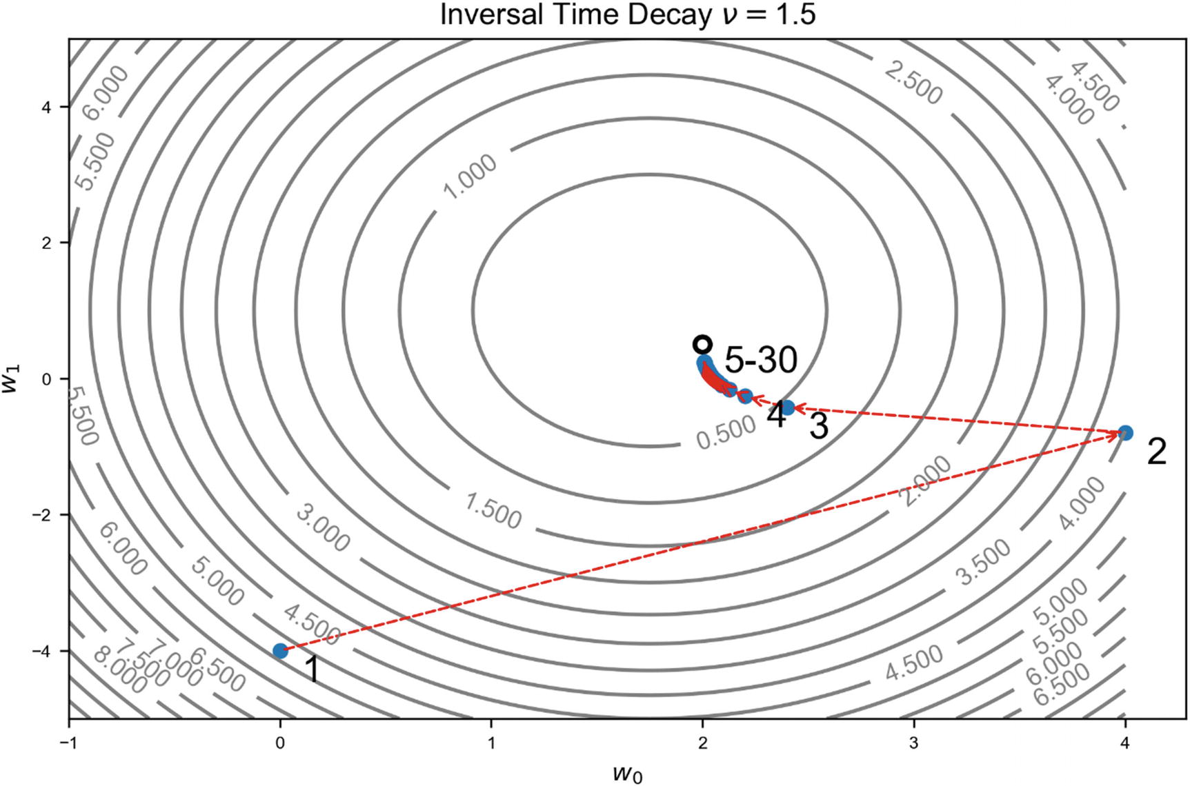
It is very interesting to see what happens if we choose a bigger value for ν. In Figure 4-7, the initial learning rate of γ0 = 2 has been chosen, and an inverse time decay algorithm with ν = 1.5 has been used. The different estimates wn are indicated with points. The minimum is indicated by the circle approximately in the middle of the image. The algorithm is now able to converge. Each point has been labeled with the iteration number, to make following the weights update easier.
Figure 4-7
Illustration of the gradient descent algorithm for ν = 1.5
What we observe in Figure 4-7 makes perfect sense. Increasing ν makes the learning rate decrease faster, and, therefore, more steps are required to reach the minimum, because the learning rate is increasingly smaller, in comparison to what happens in Figure 4-6. We can compare the behavior of the cost functions for the two values of ν. In Figure 4-8, you can see in plot (A) the cost function vs. the number of epochs. At first sight, the two seem to converge equally as fast. But let’s zoom around J = 0 in plot (B). You can clearly see how with ν = 0.2 the convergence is much faster, because the learning rate is bigger than for ν = 1.5.
Figure 4-8
Cost function vs. the number of epochs. In plot (A), the entire range of values that the cost functions assume are plotted. In plot (B), the area around J = 0 has been zoomed in to show how the cost functions decrease much faster for smaller values of ν.
Table 4-3
Additional Hyperparameters Introduced
Hyperparameter
Example
Decay rate v
v = 0.2
Exponential Decay
Another way of reducing the learning rate is according to the formula called exponential decay
See Figure 4-9 to get an idea of the speed of the learning rate. Note that the y axis has been plotted in logarithmic scale, to make the entity of the changes easier to compare. Note how for ν = 0.01, after 200 iterations (not epochs), the learning rate is already a factor 1000 smaller than that at the start!
Figure 4-9
Decrease in the learning rate for three values of ν: 0.01, 0.1, and 0.8, and T = 100, using the exponential decay algorithm
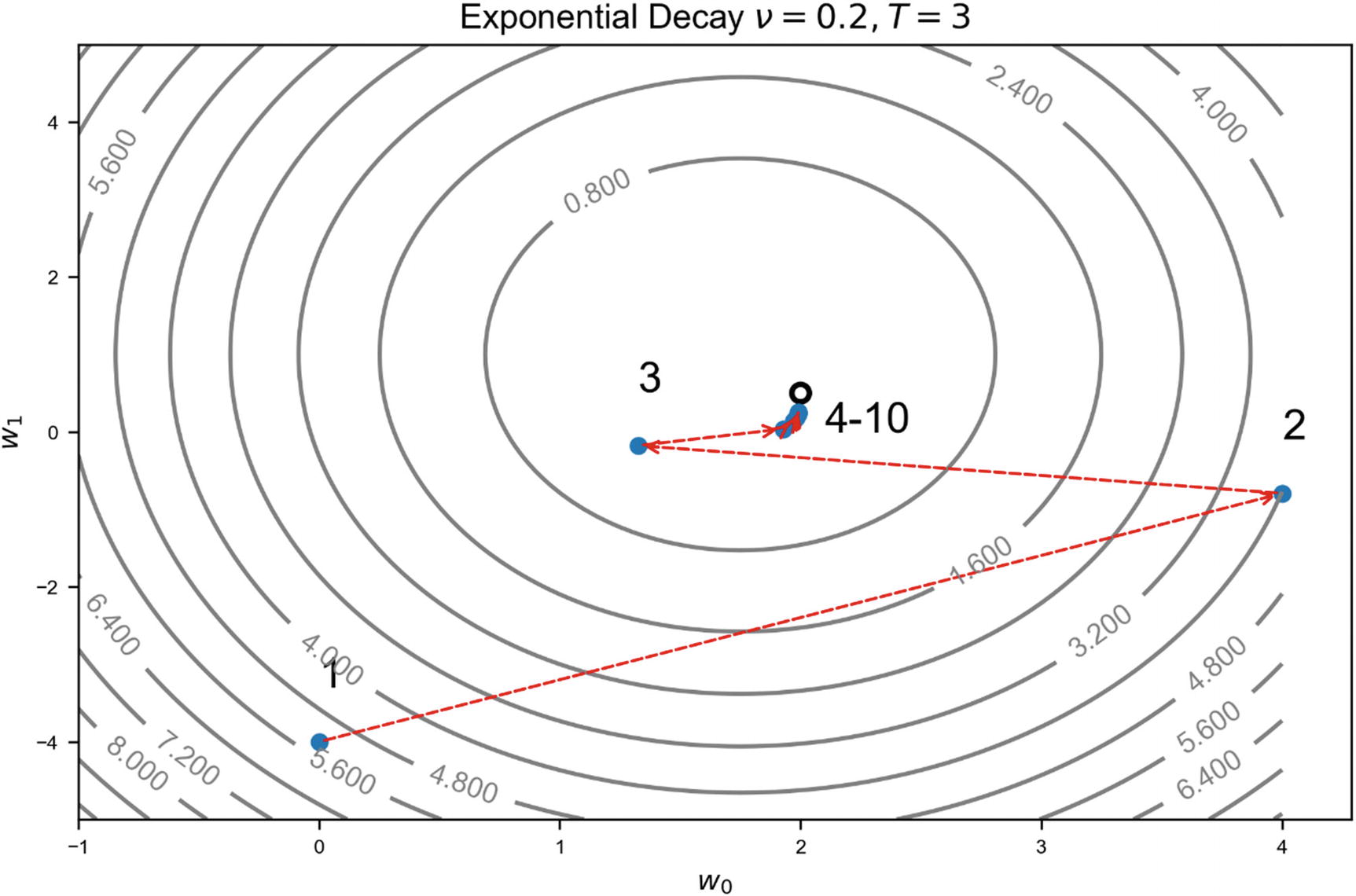
We can apply this method to our problem with ν = 0.2 and T = 3 and, again, the algorithm converges. In Figure 4-10, the initial learning rate of γ0 = 2 has been chosen, and an exponential decay algorithm with ν = 0, 2 and T = 3 has been used. The different estimates wn are indicated with points. The minimum is indicated by the circle approximately in the middle of the image. The algorithm is now able to converge. Each point has been labeled with the iteration number, to make following the weights update easier.
Figure 4-10
Illustration of the gradient descent algorithm for exponential decay
Table 4-4
Additional Hyperparameters Introduced
Hyperparameter
Example
Decay rate v
v = 0.2
Decay steps T
T = 3
Natural Exponential Decay
Another way of reducing the learning rate is according to the formula called natural exponential decay
This case is particularly interesting because it allows you to learn a few important things. Consider first Figure 4-11, to compare how different values of ν relate to different decreases in speed for the learning rate.
Figure 4-11
Decreased learning rate for three values of ν: 0.01, 0.1, and 0.8 and T = 100, using the natural exponential decay algorithm. Note that the y axis has been plotted in logarithmic scale, to make the entity of the changes easier to compare. Note how for ν = 0.8 after 200 iterations (not epochs), the learning rate is already a factor 1064 smaller than that at the start.
I would like to draw your attention to the values on the y axis (note that it is using a logarithmic scale). For ν = 0.8 after 200 iterations, the learning rate is a factor of 10−64 of the initial value! Practically zero. That means that already after a few iterations, no more updates can occur, because the learning rate is too small. To give you an idea of the scale of 10−64, a hydrogen atom is “only” roughly 10−11m! So, unless you are very careful with the choice of ν, you will not get very far.
Consider Figure 4-12, for which I have plotted our weights, as they are updated with the GD algorithm, for two values of the learning rate: 0.2 (dotted) and 0.5 (continuous).
Figure 4-12
Illustration of the gradient descent algorithm with natural exponential decay
To check the convergence, we need to zoom in around the minimum. You’ll see that in Figure 4-13. In case you are wondering why the minimum seems to be in a different position relative to the contour lines as in Figure 4-12, this is because the contour lines are not the same, because in Figure 4-13, we are much closer to the minimum.
Figure 4-13
Illustration of the gradient descent algorithm zoomed in around the minimum. The same method and parameters used in Figure 4-12 have been used here.
Now we see something that makes again sense. The continuous line is for ν = 0.5; therefore, the learning rate decreases much faster and does not manage to reach the minimum. In fact, after only 7 iterations, we have γ = 0.06, and after 20 iterations, we have γ = 9 · 10−5, a value so small that the convergence no longer manages to proceed at a reasonable speed! Again, it is very instructive to check the cost function decrease for the two parameters (see Figure 4-14).
Figure 4-14
Cost function vs. the number of epochs for natural exponential decay for two values of ν = 0.2 and 0.5. In plot (A), the entire range of values that the cost functions assume are plotted. In plot (B), the area around J = 0 has been zoomed in to show how the cost functions decrease much faster for smaller values of ν.
We see with plot (B) how the cost function for ν = 0.5 does not reach zero and becomes practically constant, because the learning rate is too small. You may think that by using more iterations, the method will eventually converge, but that is not the case. Refer to Figure 4-15 to see that the convergence process actually stops, owing to the learning rate being almost zero after a while. In the figure, the initial learning rate of γ0 = 2 has been chosen, and an exponential decay algorithm with ν = 0.5 has been used. The GD does not manage to reach the minimum. The different estimates wn are indicated with points. The minimum is indicated by the circle approximately in the middle of the image. The algorithm is now able to converge. Each point has been labeled with the iteration number, to make following the weights update easier.
Figure 4-15
Illustration of the gradient descent algorithm zoomed in around the minimum for 200 iterations
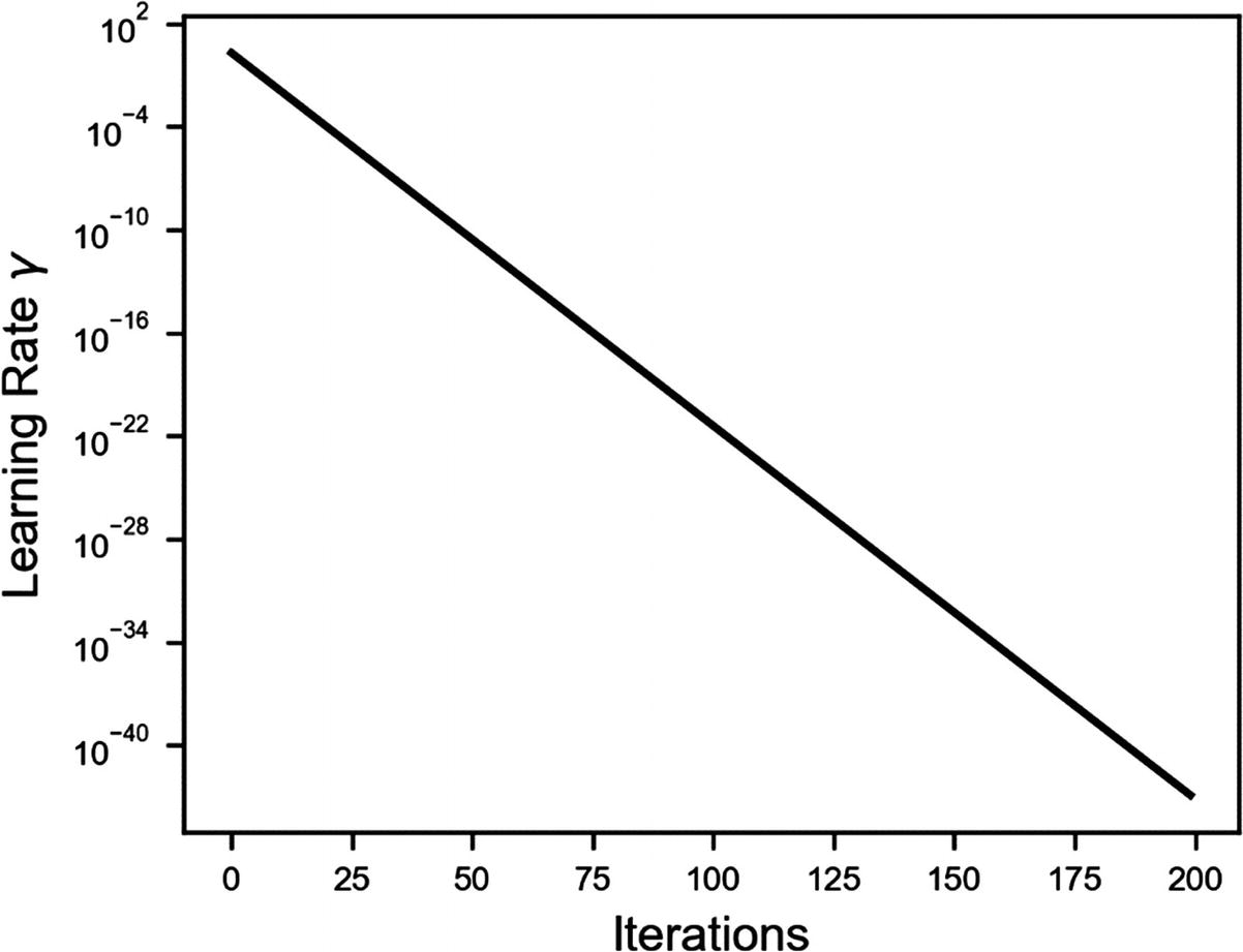
Let’s check the learning rate during this process for ν = 0.5 (see Figure 4-16). Check the values along the y axis. The learning rate reaches 10−40 after roughly 175 iterations. For all practical purposes, it is zero. The GD algorithm will not update the weights anymore, regardless of how many iterations you let it run.
Figure 4-16
Learning rate vs. the number of iterations with natural exponential decay for ν = 0.5. Note that the y axis is in logarithmic scale, to better highlight the change of γ.
To finish, let’s compare the methods by putting them on the same plot, to get an idea of the relative behavior. In Figure 4-17, you can see three plots tracking the learning rate decay for each method with different parameters.
Figure 4-17
Comparison of different parameters of the learning rate decay for the algorithm indicated
Note
You should be aware of how fast your learning rate is decreasing, to avoid it becoming practically zero and stopping your convergence altogether.
tensorflow Implementation
I should briefly talk about how tensorflow implements the methods I just explained, because there are a few details that you should know. In tensorflow, you can find the following functions to perform dynamic learning rate decay:2
Polynomial decay is a slightly more complex way of decreasing the learning rate. This had not been discussed, because it is rarely used, but you can read the documentation on the TensorFlow web site, to get an idea of how it works.
TensorFlow uses an additional parameter to give you a bit more flexibility. Take, for example, the inverse time decay method. Our equation for the learning rate decay was
where we have two parameters: γ0 and ν. TensorFlow uses three parameters:
where νds is called in TensorFlow code decay_step. The formula you will find in the TensorFlow official documentation in Python code is
to link TensorFlow language with our notation, as follows:
global_step → j (number of iterations)
decay_rate → ν
decay_step → νds
learning_rate → γo (initial learning rate)
You may ask yourself why you want to have this additional parameter. The parameter, mathematically speaking, is redundant. We can simply set our ν to the same value of ν/νds, and we would get the same result. The problem, practically, is that j (the number of iterations) gets very big very quickly, and, therefore, our ν may need to assume very small values, to be able to get a reasonable learning rate decrease. The goal of the parameter νds is to scale the number of iterations. For example, you can set this parameter to νds = 105, thereby making the decrease of the learning rate occur on a scale of 105 iterations, instead of every single iteration. If you have a huge dataset with 108 observations, and you use a mini-batch size of 50, you will get 2 · 106 iterations for each epoch. Suppose you then want your learning rate to be 1/5 of the initial value after 100 epochs. For this, you would need a ν = 2 · 10−8, a rather small value that, more important, depends on the size of your dataset and the mini-batch size. If you “normalize,” so to speak, the number of iterations, you can choose a value for ν that can remain constant, if you choose to change, for example, the mini-batch size. There is an additional practical reason (more important than that I just discussed), which is the following: the tensorflow function has an additional parameter: staircase, which can assume the values of True or False. If set to True, the following function is used:
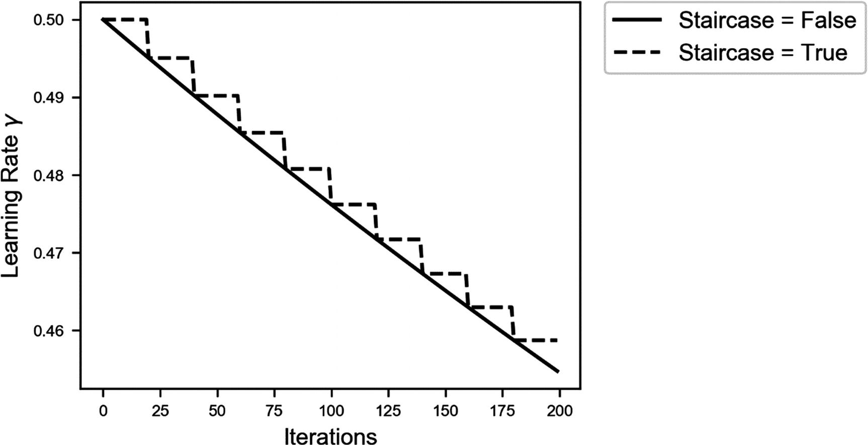
And, therefore, you get an update only for each νds iteration, instead of continuously. In Figure 4-18, you can see the difference for ν = 0.5 and νds = 20 for 200 iterations. You may want to keep your learning rate constant for ten epochs before updating it.
Figure 4-18
Learning rate decay with the two variations obtained with tensorflow with staircase = True and False
The same parameters are needed by the functions tf.train.inverse_time_decay, tf.train.natural_exp_decay, and tf.train.polynomial_decay. They work in the same way, and the purpose of the additional parameter is what I just described. Don’t be confused when implementing the methods in tensorflow, if you need this additional parameter. I will show you how to implement it for inverse time decay, but it works in the same exact way for all the other types. You need the following additional lines of code:
The only difference is the additional parameter in the minimize function: global_step = global_step. The minimize function will update the global_step variable with the iteration number with each update. That’s all. It works in the same way for the other functions.
The only difference is for the function piecewise_constant, which requires different parameters: x, boundaries, and values. For example (from the TensorFlow documentation):
…use a learning rate that’s 1.0 for the first 100000 steps, 0.5 for steps 100001 to 110000, and 0.1 for any additional steps
This would require
boundaries = [100000, 110000]
values = [1.0, 0.5, 0.1]
The code
boundaries = [b1,b2,b3, ..., bn]
values = [l1,l12,l23,l34, ..., ln]
will give a learning rate of l1 before b1 iterations, l12 between b1 and b2 iterations, l23 between b2 and b3 iterations, and so on. Keep in mind that with this method, you must set manually all the values and boundaries in the code. This will require quite some patience, if you want to test each combination to see whether it is working well. An implementation of the step decay algorithm in TensorFlow would look like this:
Let’s try to apply the methods you just learned to a realistic scenario. For this, we will employ the Zalando dataset used in Chapter 3. Please check Chapter 3 again, to see how to load the dataset and how to prepare the data. At the end of the chapter, we wrote the functions to construct a model with many layers and a function to train it. Let’s consider a model with 4 hidden layers, each containing 20 neurons. Let’s compare how the model learns with a starting initial learning rate of 0.01, keep that constant, and then apply the inverse time decay algorithm, starting with a γ0 = 0.1, ν = 0.1, and νds = 103 (see Figure 4-19).
Figure 4-19
Cost function behavior for a neural network of 4 layers, each having 20 neurons, applied to the Zalando dataset. The continous line is for a model with a constant learning rate of γ = 0.01. A dashed line is for a network in which we have used the inverse time decay algorithm, with a γ0 = 0.1, ν = 0.1, and νds = 103.
So, even with a starting learning rate ten times larger, the algorithm is much more efficient. Is has been proven in several research papers that applying a dynamic learning rate makes learning faster and more efficient, as we have noted in this case.
Note
Unless you are using optimization algorithms that include a learning rate change during training (you will see them in the next sections), it is generally a good idea to use dynamic learning rate decay. This makes learning stable and usually faster. The downside is that you have more hyperparameters to tune.
Normally, it is a good idea, when using dynamic learning rate decay, to start with an initial learning rate γ0 bigger than you would normally use. Because γ is decreasing, this won’t normally create problems and will make the convergence at the beginning (one hopes) faster. As you should now expect, there are no fixed rules on which method works better. Each case and dataset is different, and some testing is always required, to see which parameter value yields the best results.
Common Optimizers
Until now, we have used gradient descent to minimize our cost function. That is not the most efficient way to proceed, and there are some modifications to the algorithm that can make it much faster and more efficient. This is a very active area of research, and you will find an incredible number of algorithms, based on different ideas, to make the learning faster. I will cover here the most instructive and well-known ones: Momentum, RMSProp, and Adam. Additional material that you can consult to investigate the most exotic algorithms has been written by S. Ruder, in a paper titled An overview of gradient descent optimization algorithms (available at https://goo.gl/KgKVgG). The paper is not for beginners and requires an extensive mathematical background, but it gives an overview of such unusual algorithms as Adagrad, Adadelta, and Nadam. Additionally, it reviews weights update schemes applicable in distributed in such environments as Hogwild!, Downpour SGD, and many more. Surely, it is a read worth your time.
To understand the basic idea of Momentum (and partially, too, RMSProp and Adam), you first must understand what exponentially weighted averages are.
Exponentially Weighted Averages
Let’s suppose that you are measuring a quantity θ (it could be the temperature where you live) over time—once a day, for example. You will have a series of measurements that we can indicate with θi, where i goes from 1 to a certain number N. Bear with me, if, at the beginning, this does not make much sense; however, let’s define recursively a quantity vn as
and so on, with β, a real number with 0 < β < 1. Generally, we could write the nth term as
Now let’s write all the terms, v1, v2, and so on, just as a function of β and θi (so, not recursively). For v2, we have
for v3,
Generalizing, we obtain
Or, more elegantly (without the three dots),
Now let’s try to understand what this formula means. First, note that the term βn disappears if we choose v0 = 0. Let’s do that (we set v0 = 0) and consider now what remains:
Are you still with me? Now comes the interesting part. Let’s define the convolution between two sequences.3 Consider two sequences: xn and hn. The convolution between the two (which we indicate with the symbol ∗) is defined by
Now, because we have only a finite number of measurements for our quantity θi, we will have
Therefore, we can write vn as a convolution as
where we have defined
To get an idea of what that means, let’s plot together θn, bn, and vn. To do this, let’s assume that θn has a Gaussian shape (the exact form is not relevant, it is only for illustrative purposes), and let’s take β = 0.9 (see Figure 4-20).
Figure 4-20
A plot (left) showing θn (solid line) and bn (dotted line) together, and one (right) showing the points that must be summed to obtain vn for n = 50
Now I’ll discuss briefly Figure 4-20. The Gaussian curve (θn) will be convoluted with bn to obtain vn. The result can be seen in the plot at right. All those terms, (1 − β)βn − iθi for i = 1, …, 50 (plotted at right), will be summed to obtain v50. Intuitively, vn is the average of all θn for n = 1, …, 50. Each term is then multiplied by a term (bn) that is 1 for n = 50 and then decreases rapidly for n, decreasing toward 1. Basically, this is a weighted average, with an exponentially decreasing weight (thus the name). The terms farther from n = 50 are less and less relevant, while the terms close to n = 50 get more weight. This is also a moving average. For each n, all the preceding terms are added, each multiplied by a weight (bn).
I would like now to show you why there is this factor 1 − β in bn. Why not choose only βn? The reason is very simple. The sum of bn over all positive n is equal to 1. Let’s see why. Consider the following equation:
where we have used the fact that for β < 1, we have , and that for a geometric series, we have
The algorithm we described to calculate vn is nothing else than the convolution of our quantity θi, with a series the sum of which is equal to 1 and has the form (1 − β)βi.
Note
The exponentially weighted average vn of a series of a quantity θn is the convolution vn = θn ∗ bn of our quantity θi, with bn = (1 − β)βn, where bn has the property that its sum over the positive values of n is equal to 1. It has the intuitive meaning of a moving average, in which each term is multiplied by weights given by the sequence bn.
As you choose β smaller and smaller, the number of points θn that have a weight significantly different from zero decreases, as you can see in Figure 4-21, in which the series bn for different values of β is plotted.
Figure 4-21
The series bn for three values of β: 0.9, 0.8, and 0.3. Note that as β gets smaller, the series is significantly different from zero for an increasingly smaller number of values around n = 0.
This method is at the very core of the Momentum optimizer and more advanced learning algorithms, and you will see in the next sections how it works in practice.
Momentum
You will remember that in plain gradient descent, the weights updates are calculated with the equations
The idea behind the Momentum optimizer is to use exponentially weighted averages of the corrections of the gradient and then use them for the weights updates. More mathematically we calculate
and we will then perform the updates with the equations
where usually vw, [0] = 0 and vb, [0] = 0 are chosen. That means, as you can now understand from the discussion about exponentially weighted averages from the previous section, that instead of using the derivatives of the cost functions with respect to the weights, we update the weights with a moving average of the derivatives. Usually, experience shows that a bias correction could theoretically be neglected.
Note
The Momentum algorithm uses an exponential weighted average of the derivatives of the cost function with respect to the weights for the weights updates. In this way, not only the derivatives at a given iteration are used, but also the past behavior is considered. It may happen that the algorithm oscillates around the minimum, instead of converging directly. This algorithm can escape from plateaus much more efficiently than standard gradient descent.
Sometimes, you find in books or blogs a slightly different formulation (I provide here only the equation for the weights, w, for brevity).
The idea and meaning remain the same. It is simply a slightly different mathematical formulation. I find that the method I described is easier to understand intuitively with the notion of sequence convolution and of weighted averages than this second formulation. Another formulation that you will find (and one that TensorFlow uses) is
where ηt is called by TensorFlow Momentum (the superscript t indicates that this variable is used by TensorFlow). In this formulation, the weight update assumes the form
where, again, the superscript t indicates that the variable is the one used by TensorFlow. Although it seems different, this formulation is completely equivalent to the formulation I gave you at the beginning of this section.
The TensorFlow formulation and the one I discussed previously are equivalent, if we choose
That can be seen by simply comparing the two different equations for the weights updates. Typically, values around η = 0.9 in TensorFlow implementations are used, and they generally work well.
Implementing Momentum in TensorFlow is extraordinarily easy. Just replace the GradientDescentOptimizer with tf.train.MomentumOptimizer(learning_rate = learning_rate, momentum = 0.9).
The Momentum almost always converges faster than plain gradient descent.
Note
Comparing the different parameters in the different optimizers is wrong. The learning rate, for example, has a different meaning in the different algorithms. What you should compare is the best convergence speed you can achieve with several optimizers, regardless of the choice of parameters. Comparing the GD for a learning rate of 0.01 with Adam (covered later) for the same learning rate does not make much sense. You should compare the optimizers with the parameters that give you the best and fastest convergence, to decide which one to use.
In Figure 4-22, you can see the cost function for the problem discussed in the previous section for plain gradient descent (with γ = 0.05) and for Momentum (with γ = 0.05 and η = 0.9). You can see how the Momentum optimizer oscillates around the minimum. What is difficult to see on the y scale is that with Momentum, J reaches a much lower value.
Figure 4-22
Cost function vs. the number of epochs for plain gradient descent (with γ = 0.05) and for Momentum (with γ = 0.05 and η = 0.9). You can see how the Momentum optimizer oscillates a bit around the minimum.
More interesting is to check how the Momentum optimizer chooses its path along the cost function surface. In Figure 4-23, you can see a 3D surface plot of the cost function. The continuous line is the path that the gradient descent optimizer chooses, along the maximum steepness, as expected. The dashed line is the one that the Momentum optimizer chooses as it oscillates around the minimum.
Figure 4-23
3D surface plot of the cost function J. The continuous line is the path that the gradient descent optimizer chooses—along the maximum steepness, as expected. The dashed line is the one that the Momentum optimizer chooses as it oscillates around the minimum.
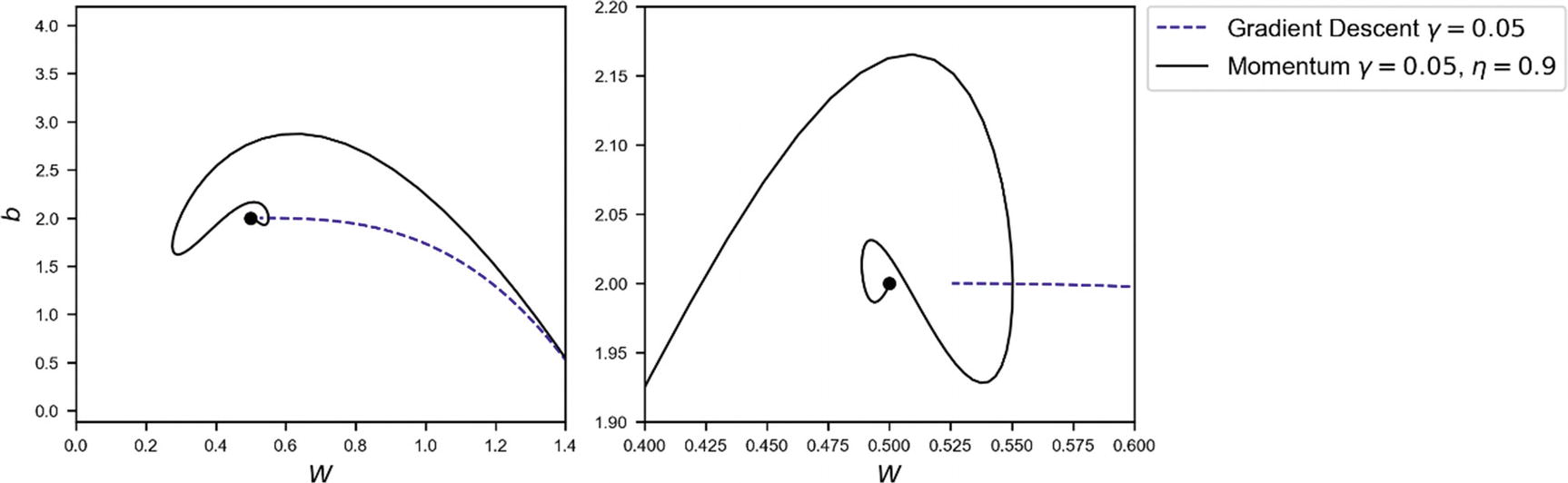
I want to convince you that Momentum is faster and better at converging. To do that, let’s check in the weights plane how the two optimizers behave. In Figure 4-24, you can see the path that the two optimizers have chosen. On the right plot, you can see a zoom around the minimum. You can see how gradient descent after 100 epochs does not manage to reach the minimum, although it seems to choose a more direct path toward the minimum. It gets very close, but not close enough. The Momentum optimizer oscillates around the minimum and reaches it very efficiently.
Figure 4-24
Path that the two optimizers have chosen. The right plot shows a zoom around the minimum. You can see how Momentum reaches the minimum after oscillating around it, while GD does not manage to reach it in 100 epochs.
RMSProp
Let’s move to something a bit more complex, but usually more efficient. Let me give you the mathematical equations, and then we will compare them to the others we have seen so far. At each iteration, we need to calculate
where the symbol ∘ indicates an element-wise product. Then we will do the update of our weights with the equations
So, first you determine an exponential weighted average of the quantities Sw, [n + 1] and Sb, [n + 1] and then use them to modify the derivatives that you use to do your weights updates. The ϵ, usually ϵ = 10−8, is there to avoid the denominator going to zero in case the quantities Sw, [n + 1] and Sb, [n + 1] go to zero. The intuitive idea is that if the derivative is big, then the S quantities are big; therefore, the factors or will be smaller and the learning will slow down. The reverse is also true, so if the derivatives are small, the learning will be faster. This algorithm will make the learning faster for the parameters that are slowing it down. In TensorFlow, it is again particularly easy to use it simply with the following code:
Let’s check what path this optimizer chooses. In Figure 4-25, you can see that RMSProp oscillates around the minimum. While the GD does not reach it, the RMSProp algorithm has time to do several loops around it before reaching it.
Figure 4-25
Path chosen toward the cost function minimum by plain gradient descent and RMSProp. The latter makes loops around the minimum and then reaches it. In the same number of epochs, the GD does not even get that close. Note the scale of the plot on the right. The zoom level is very high. We are looking at an extreme close-up (the GD path is not even visible on this scale) around the minimum.
In Figure 4-26, you can see in 3D the same path along the cost function surface.
Figure 4-26
Path choosen by the GD (γ = 0.05) and RMSProp (γ = 0.05, η = 0.9, ϵ = 10−10) along the surface of the cost function. The red dot indicates the minimum. RMSProp, especially at the beginnig, chooses a more direct path toward the minimum than GD.
In Figure 4-27, you can see GD, RMSProp and Momentum paths. You can see how the RMSProp path is much more direct toward the minimum. It gets close to it very quickly and then oscillates closer and closer. It overshoots a bit at the beginning but then corrects itself quickly and comes back.
Figure 4-27
Path toward the minimum choosen by GD, RMSProp, and Momentum. You can see how the RMSProp path toward the minimum is much more direct. It gets around it very quickly and then oscillates closer and closer.
Adam
The last algorithm we will look at is called Adam (Adaptive Moment estimation). It combines the ideas of RMSProp and Momentum in one optimizer. Like Momentum, it uses an exponential weighted averages of past derivatives, and like RMSProp, it uses the exponentially weighted averages of past squared derivatives.
You will have to calculate the same quantities that you need for Momentum and for RMSProp, and then you must calculate the following quantities:
Similarly, you must calculate
Where we have used β1 for the hyperparameter, we will use it in Momentum and β2 for the one we used in RMSProp. Then, as we did in RMSProp, we will update our weights with the equations
TensorFlow does everything for us, if we simply use the following line:
where, in this case, the typical values for the parameters have been chosen: γ = 0.3, β1 = 0.9, β2 = 0.999, and ϵ = 10−8. Note that because this algorithm adapts the learning rate to the situation, we can start with a bigger learning rate, to speed up the convergence.
In Figure 4-28, you can see the path around the minimum chosen by GD and the Adam optimizer. Adam, too, oscillates around the minimum, but it reaches it without problems. On the right plot (a zoom around the minimum), you can see how the algorithm gets very close to the minimum. To give you an idea of how good the optimizer is, after just 200 epochs, the weights and bias get to 0.499983, 2.000047, which is really close to the minimum (remember that the minimum is at w = 0.5 and b = 2.0).
Figure 4-28
Path that GD and Adam optimizers choose after 200 epochs. Note the amount of loops that Adam takes around the minimum. Regardless, the opimizer is really efficient compared to the plain GD.
I haven’t shown you all the optimizers together, since you would see a lot of loops, and that would not really teach you anything.
Which Optimizer Should I Use?
In short, you should use Adam. It is generally considered faster and better than other methods. This does not mean that is always the case. There are recent research papers that indicate how these optimizers could generalize poorly on new datasets (see, for example, Ashia C. Wilson, Rebecca Roelofs, Mitchell Stern, Nathan Srebro, and Benjamin Recht, “The Marginal Value of Adaptive Gradient Methods in Machine Learning,” at https://goo.gl/Nzc8bQ). And there are other papers that endorse use of GD with a dynamical learning rate decay. It mostly depends on your problem. But, generally, Adam is a very good starting point.
Note
If you are unsure about which optimizer to start with, use Adam. It is generally considered faster and better than other methods.
To give you an idea of how good Adam can be, let’s apply it to the Zalando dataset. We will use a network with 4 hidden layers, each with 20 neurons. The model we will use is the one discussed at the very end of Chapter 3. Figure 4-29 shows how the cost function converges faster when using Adam optimization, compared to GD. Additionally, in 100 epochs, GD reaches an accuracy of 86%, while Adam reaches 90%. Note that I have not changed anything in the model, except the optimizer! For Adam, I have used the following code:
Cost function of the Zalando dataset for a network with 4 hidden layers, each with 20 neurons. The continous line is plain GD, with a learning rate of γ = 0.01, and the dashed line is Adam optimization, with γ = 0.1, β1 = 0.9, β2 = 0.999, and ϵ = 10−8.
As I suggested, when testing complex networks on big datasets, the Adam optimizer is a good place to start. But you should not limit your tests only to this optimizer. A test of other methods is always worthwhile. Perhaps another approach will work better.
Example of Self-Developed Optimizer
Before completing this chapter, I want to show you how to develop your own optimizer, using TensorFlow. This is very useful when you want to use an optimizer that is not directly available. Take, for example, the paper from Neelakantan et al.4 In their research, they show how adding random noise to the gradients when training complex networks allows plain gradient descent to become very effective. They show how a 20-layer deep network can be trained efficiently with standard GD, even starting with poor weight initialization.
If you want to test this method, for example, you cannot use the tf.GradientDescentOptimizer function, because this implements a plain GD, without the noise described in the paper. To test it, you must have access to the gradients in the code, add the noise to them, and then update the weights with the modified gradients. We will not test their method here; that would require too much time and would go beyond the scope of this book, but is instructive to see how to develop plain gradient descent without using the tf.GradientDescentOptimizer and without calculating any derivative manually.
Before constructing our network, we must know the dataset we want to use and what problem (regression, classification, etc.) we want to solve. Let’s make something new with a known dataset. Let’s use the MNIST dataset we used in Chapter 2, but this time, lets perform multiclass classification using the softmax function, as we did on the Zalando dataset in Chapter 3. In Chapter 2, I discussed at length how to load the MNIST dataset with sklearn, so let’s do it in a different (and more efficient) way here. TensorFlow has a method to download the MNIST dataset, including labels already one-hot encoded. This can be done simply with the following lines:
from tensorflow.examples.tutorials.mnist import input_data
You will find the files in the folder (if you are using Windows) c: mpdata. If you want to change the location where the files are stored, you must change the "/tmp/data" parameter of the function read_data_sets. Now, as you probably remember from Chapter 2, the MNIST images are 28 × 28 pixels (784 pixels in total) images, in grayscale, so each pixel can assume a value from 0 to 254. Having this information, we can now construct our network.
X = tf.placeholder(tf.float32, [784, None]) # mnist data image of shape 28*28=784
The preceding code gives you the tensors that contain the gradients of the cost node with respect to W and b, respectively. TensorFlow calculates them for you automatically! If you are interested to know how, check the official documentation of the tf.gradients function at https://goo.gl/XAjRkX. Now we must add nodes to the computational graph that updates the weights, and that is what we do with the lines
new_W = W.assign(W - learning_rate_ * grad_W)
new_b = b.assign(b - learning_rate_ * grad_b)
When we ask TensorFlow to evaluate the nodes new_W and new_b during our session, the weights and bias get updated. Finally, we must modify the function that evaluates the graph, using (for the mini-batch GD) the line
In this way, the new nodes new_W and new_b get evaluated, and, in doing so, TensorFlow updates the weights and bias. The following lines are no longer required:
This function is slightly different than those we have used before, because here, I used some features of TensorFlow to make our life a bit easier. In particular, the line
calculates the total number of mini-batches that we have, because the variable mnist.train.num_examples contains the number of observations we have at our disposal. Then to get the batches, we use
This returns two tensors, containing the training input data (batch_xs) and the one-hot encoded labels (batch_ys). We then simply have to transpose them, because TensorFlow returns the array with observations as rows. We do that with the lines
batch_xs_t = batch_xs.T
batch_ys_t = batch_ys.T
I also added to the function the accuracy calculation, to make it easier to see how well we are doing. Letting the model run with the python call
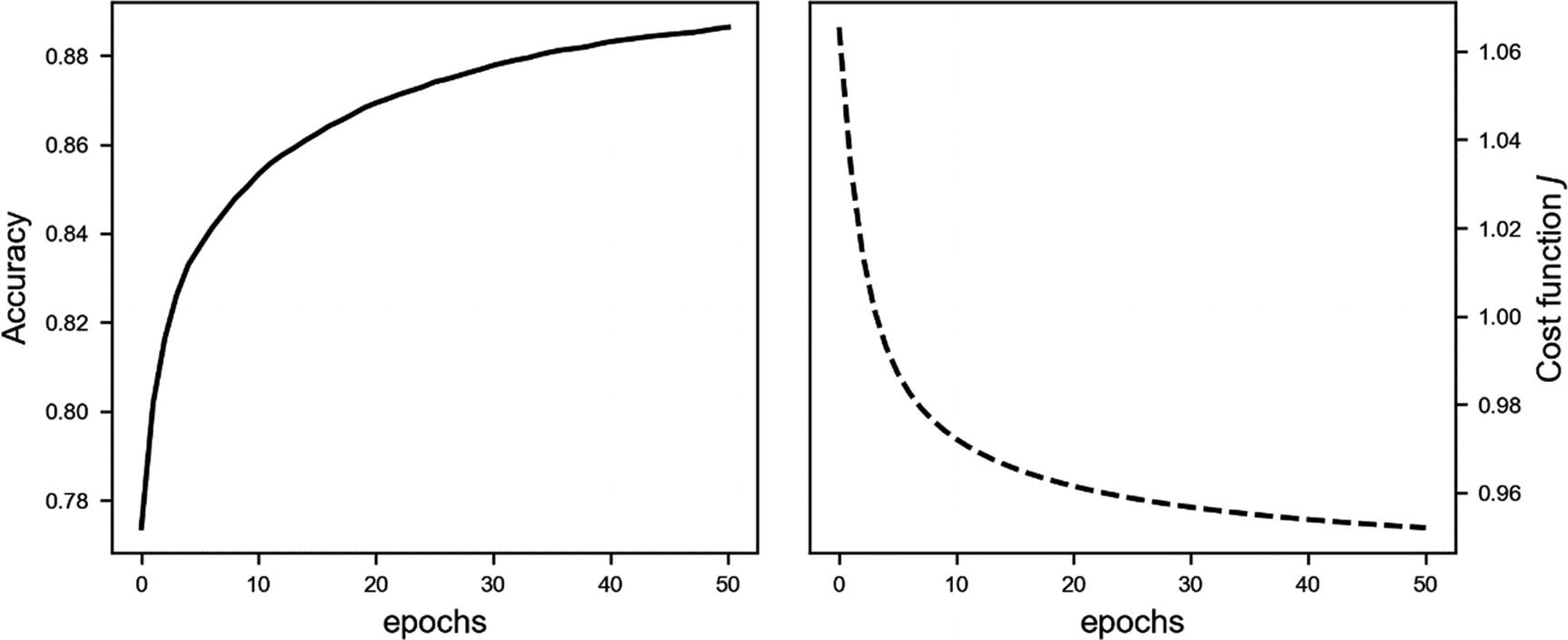
This model will work exactly as the one with the gradient descent optimizer provided by TensorFlow. But now, you have access to the gradients, and you can modify them, add noise to them (if you want to try), and so on. In Figure 4-30, you can see the cost function behavior (on the right side) and the accuracy vs. the epochs (on the left side) that we get with this model.
Note
TensorFlow is a great library, because it gives you the flexibility to build your models basically from scratch. But it is important to understand how the different methods work, to be able to use the library to its fullest. You need to have a very good understanding of the mathematics behind the algorithms, to be able to tune them or to develop variations.
Figure 4-30
Cost function behavior (right) and the accuracy vs. epochs (left) for the neural network with one neuron and with the gradient descent developed with the tf.gradients function
![$$ {w}_{0,left[n+1
ight]}={w}_{0,left[n
ight]}-gamma frac{partial Jleft({w}_{0,left[n
ight]},{w}_{1,left[n
ight]}
ight)}{partial {w}_0} $$](http://images-20200215.ebookreading.net/10/2/2/9781484237908/9781484237908__applied-deep-learning__9781484237908__images__463356_1_En_4_Chapter__463356_1_En_4_Chapter_TeX_Equa.png)
![$$ {w}_{1,left[n+1
ight]}={w}_{1,left[n
ight]}-gamma frac{partial Jleft({w}_{0,left[n
ight]},{w}_{1,left[n
ight]}
ight)}{partial {w}_1} $$](http://images-20200215.ebookreading.net/10/2/2/9781484237908/9781484237908__applied-deep-learning__9781484237908__images__463356_1_En_4_Chapter__463356_1_En_4_Chapter_TeX_Equb.png)


![$$ gamma =frac{gamma_0}{1+
u left[frac{j}{
u_{ds}}
ight]} $$](http://images-20200215.ebookreading.net/10/2/2/9781484237908/9781484237908__applied-deep-learning__9781484237908__images__463356_1_En_4_Chapter__463356_1_En_4_Chapter_TeX_Equk.png)


 , and that for a geometric series, we have


![$$ {v}_{w,left[n+1
ight]}=gamma {v}_{w,left[n
ight]}+eta {
abla}_{mathbf{w}}Jleft({w}_{left[n
ight]},{b}_{left[n
ight]}
ight) $$](http://images-20200215.ebookreading.net/10/2/2/9781484237908/9781484237908__applied-deep-learning__9781484237908__images__463356_1_En_4_Chapter__463356_1_En_4_Chapter_TeX_Equab.png)
![$$ {v}_{w,left[n+1
ight]}={eta}^t{v}_{w,left[n
ight]}+{
abla}_{mathbf{w}}Jleft({w}_{left[n
ight]},{b}_{left[n
ight]}
ight) $$](http://images-20200215.ebookreading.net/10/2/2/9781484237908/9781484237908__applied-deep-learning__9781484237908__images__463356_1_En_4_Chapter__463356_1_En_4_Chapter_TeX_Equac.png)
![$$ {w}_{left[n+1
ight]}={w}_{left[n
ight]}-{gamma}^t{v}_{w,left[n+1
ight]}={w}_{left[n
ight]}-{gamma}^tleft({eta}^t{v}_{w,left[n
ight]}+{
abla}_{mathbf{w}}Jleft({w}_{left[n
ight]},{b}_{left[n
ight]}
ight)
ight)={w}_{left[n
ight]}-{gamma}^t{eta}^t{v}_{w,left[n
ight]}-{gamma}^t{
abla}_{mathbf{w}}Jleft({w}_{left[n
ight]},{b}_{left[n
ight]}
ight) $$](http://images-20200215.ebookreading.net/10/2/2/9781484237908/9781484237908__applied-deep-learning__9781484237908__images__463356_1_En_4_Chapter__463356_1_En_4_Chapter_TeX_Equad.png)


![$$ 1/sqrt{S_{w,left[n+1
ight]}+epsilon } $$](http://images-20200215.ebookreading.net/10/2/2/9781484237908/9781484237908__applied-deep-learning__9781484237908__images__463356_1_En_4_Chapter__463356_1_En_4_Chapter_TeX_IEq2.png) or
or ![$$ 1/sqrt{S_{b,left[n
ight]}+epsilon } $$](http://images-20200215.ebookreading.net/10/2/2/9781484237908/9781484237908__applied-deep-learning__9781484237908__images__463356_1_En_4_Chapter__463356_1_En_4_Chapter_TeX_IEq3.png) will be smaller and the learning will slow down. The reverse is also true, so if the derivatives are small, the learning will be faster. This algorithm will make the learning faster for the parameters that are slowing it down. In TensorFlow, it is again particularly easy to use it simply with the following code:
will be smaller and the learning will slow down. The reverse is also true, so if the derivatives are small, the learning will be faster. This algorithm will make the learning faster for the parameters that are slowing it down. In TensorFlow, it is again particularly easy to use it simply with the following code: