Typically, when talking about deep learning, people think about image recognition, speech recognition, image detection, and so on. These are the most well-known applications, but the possibilities of deep neural networks are endless. In this chapter, I will show you how deep neural networks can be successfully applied to a less conventional problem: the extraction of a parameter in sensing applications. For this specific problem, we will develop the algorithms for a sensor, which I will describe later, to determine the oxygen concentration in a medium, for example, a gas.
The chapter is organized as follows: first, I will discuss the research problem to be solved, then I will explain some introductory material required to solve it, and, finally, I will show you the first results of this ongoing research project.
The Problem Description
The functioning principle of many sensor devices is based on the measurement of a physical quantity, such as voltage, volume, or light intensity, that is typically easy to measure. This quantity must be strongly correlated with another physical quantity, which is the one to be determined and, typically, difficult to measure directly, such as temperature or, in this example, gas concentration. If we know how the two quantities are correlated (typically, via a mathematical model), from the first quantity, we can derive the second, the one we are really interested in. So, in a simplified way, we can imagine a sensor as a black box, which, when given an input (temperature, gas concentration, and so on), produces an output (voltage, volume, or light intensity). The dependence of the output from the input is characteristic of the type of sensing and may be extremely complex. This makes the implementation of the necessary algorithms in real hardware very difficult, or even impossible. Here, we will use the approach to determine the output from the input, using neural networks instead of a set of formulas.
This research project deals with the measurement of oxygen concentration, using the principle of “luminescence quenching”: a sensitive element, a dye substance, is in contact with a gas, of which we want to measure the oxygen content. The dye is illuminated with a so-called excitation light (typically, in the blue part of the light spectrum) and, after absorbing a part of it, it reemits light in a different part of the spectrum (typically, in the red part). The intensity and duration of the emitted light is strongly dependent on the oxygen concentration in the gas in contact with the dye. If the gas has some oxygen in it, part of the emitted light from the dye is suppressed, or “quenched” (from here, the name of the measurement principle), this effect being strongest the higher the amount of oxygen in the gas. The goal of the project is to develop new algorithms to determine the oxygen concentration (input) from a measured signal, the so-called phase shift (output) between the exciting and emitted light. If you don’t understand what this means, don’t worry. it is not required in order for you to understand the content of this chapter. It is enough to intuitively understand that this phase shift measures the change between the light exciting the dye and the one emitted after the “quenching” effect and that this “change” is strongly affected by the oxygen contained in the gas.
The difficulty in the sensor realization is that the response of the system depends (nonlinearly) on several parameters. This dependency is, for most dye molecules, so complex that it is almost impossible to write down equations for the oxygen concentration as a function of all these influencing parameters. The typical approach is, therefore, to develop a very sophisticated empirical model, with many parameters manually tuned.
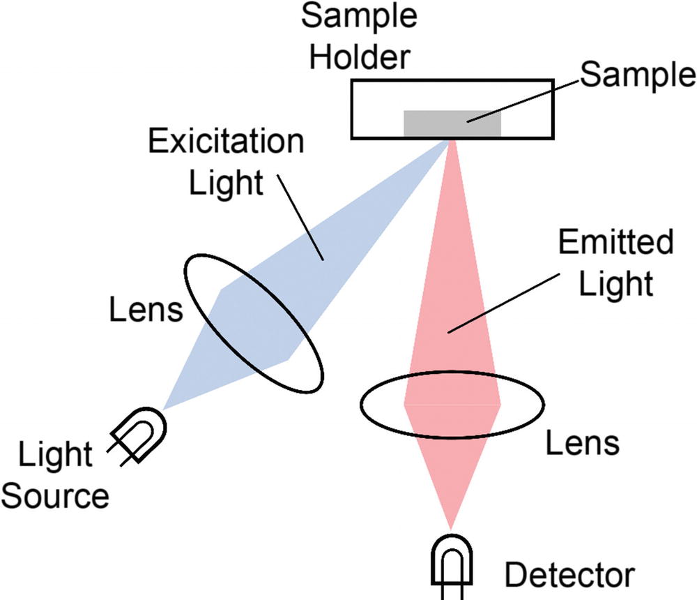
The typical setup for luminescence measurements is shown schematically in Figure 9-1. This setup was used to get the data for the validation dataset. A sample containing the luminescent dye substance is illuminated by an excitation light (the blue light in the figure), emitted by a light-emitting diode, or laser, focused with a lens. The emitted luminescence (the red light at the right of the figure) is collected by a detector with the help of another lens. The sample holder contains the dye and the gas, indicated with the sample in the figure, for which we want to measure the oxygen concentration.
Figure 9-1
Schematic setup of a luminescence measurement system
The luminescence intensity collected by the detector is not constant in time but, rather, decreases. How fast it decreases depends on the amount of oxygen present, typically quantified by a decay time, indicated with τ. The simplest description of this decay is by a single exponential decay function, e−t/τ, characterized by a decay time, τ. A common technique used in practice to determine such a decay time is to modulate the intensity of the excitation light, or, in other words, to vary the intensity in a periodic way, with a frequency f = 2πω, where ω is the so-called angular frequency. The reemitted luminescence light has an intensity that is also modulated, or, in other words, it varies periodically but is characterized by a phase shift θ. This phase shift is related to the decay time τ as tanθ = ωτ. To give you an intuitive understanding of what this phase shift is, consider the light to be represented (if you are a physicist reading this, forgive me), in its simplest form, as a wave with an amplitude varying as a trigonometric function.
The quantity θ is called the phase constant of the wave. Now what happens is that the light that excites the dye has a phase constant θexc, and the light emitted has a different phase constant, θemitted. The measurement principle measures exactly this phase change, θ ≡ θexc − θemitted, because this change is strongly influenced by the oxygen content in the gas. Please keep in mind that this explanation is highly intuitive and, from a physics point of view, not completely correct, but it should give you an approximate understanding of what we are measuring.
To summarize, the measured signal is this phase shift θ, simply called phase in the following text, while the searched quantity (the one we want to predict) is the oxygen concentration in the gas in contact with the dye.
In real life, the situation is, unfortunately, even more complicated. The light phase shift not only depends on the modulation frequency ω and the oxygen concentration O2 in the gas but also nonlinearly on the temperature and chemical composition of the surrounding of the dye molecule. Additionally, only rarely can the decay of the light intensity be described by only one decay time. Most frequently, at least two decay times are needed, further increasing the number of the parameters required to describe the system. Given a laser modulation frequency ω, a temperature T in degrees Celsius, and an oxygen concentration O2 (expressed in % of oxygen contained in air), the system returns the phase θ. In Figure 9-2, you can see a plot of a typical measured tanθ for T = 45∘C and O2 = 4%.
Figure 9-2
Plot of the measured tanθ for T = 45∘C and O2 = 4%
The idea of this research project is to be able to get the oxygen concentration from data without the need of developing any theoretical model for the behavior of the sensor. To do this, we will try to use deep neural networks and let them learn from artificially created data what the oxygen concentration in the gas is for any given phase, and then we will apply our model to real experimental data.
The Mathematical Model
Let’s look at one of the mathematical models that can be used to determine the oxygen concentration. For one thing, it gives an idea of how complicated it is, and for another, it will be used in this chapter to generate the training data set. Without going into the physics involved in the measurement technique, which is beyond the scope of this book, a simple model describing how the phase θ is linked to the oxygen concentration O2 can be described by the following formula:
The quantities f(ω, T), KSV1(ω, T), and KSV2(ω, T) are parameters whose analytical form is unknown and that are specific to the dye molecule used, how old it is, how the sensor is built, and other factors. Our goal is to train a neural network in the laboratory and later deploy it on a sensor that can be used in the field. The main problem here is to determine the frequency- and temperature-dependent function form of f, KSV1, and KSV2. For this reason, commercial sensors usually rely on polynomial or exponential approximations, with enough parameters and on fitting procedures to determine a good enough approximation of the quantities.
In this chapter, we will create the training dataset with the mathematical model just described, then we will apply it to experimental data, to see how well we can predict the oxygen concentration. The goal is a feasibility study to check how well such a method works.
Preparing the training dataset in this case is a bit tricky and convoluted, so before starting, let’s look at a similar but much easier problem, so that you get an understanding of what we want to do in the more complicated case.
Regression Problem
Let’s consider first the following problem. Given a function L(x) with a parameter A, we want to train a neural network to extract the parameter value A from a set of values of the function. In other words, given a set of values of the input variable xi for i = 1, …, N, we will calculate an array of N values Li = L(xi) for i = 1, …, N and use them as input for a neural network. We will train the network to give us as output A. As a concrete example, let’s consider the following function:
This is the so called Lorentzian function, with a maximum in x = 0 and with L(0) = 1. The problem we want to solve here is to determine A, given a certain number of data points of this function. In this case, this is rather simple, because we can do it, for example, with a classical nonlinear fit, or even by solving a simple quadratic equation, but suppose we want to teach a neural network to do that. We want a neural network to learn how to perform a nonlinear fit for this function. With all you learned in this book, this will not prove to be too difficult. Let’s start by creating a training dataset. First, let’s define a function for L(x)
def L(x,A):
y = A**2/(A**2+x**2)
return y
Let’s now consider 100 points and generate an array of all the x points we want to use.
number_of_x_points = 100
min_x = 0.0
max_x = 5.0
x = np.arange(min_x, max_x, (max_x-min_x)/number_of_x_points )
Finally, let’s generate 1000 observations, which we will use as input for our network.
data = np.zeros((number_of_samples, number_of_x_points))
targets = np.reshape(A_v, [1000,1])
for i in range(number_of_samples):
data[i,:] = L(x, A_v[i])
The array data will now contain all observations, each one on a row. Note that to avoid having negative values for A, we have built a check into the code.
if A_v[i] <= 0:
A_v[i] = np.random.random_sample([1])
In this way, if the random value chosen for A is negative, a new random value is assigned instead. You may have noticed that in the equation for L(x), the quantity A always appears squared, so on first sight, a negative value would not be a problem. But remember that this negative value will be the target variable we want to predict. When first developing this model, I had a few negative values for A. The network was not able to distinguish between positive and negative values, thus getting wrong results.
If you check the shape of the array A_v, you get
(1000, 100)
This translates as 1000 observations, each having 100 values that are the different value of L, are calculated at the values of x that we have generated. We also need a dev dataset, of course.
The model converges very fast. The MSE (the cost function) goes from 1.1 at the beginning to ca. 2.5 · 10−4 after 10,000 epochs. After 20,000 epochs, the MSE reaches 10−6. We can plot the predicted vs. the real values, to get a visual check on how the system is doing. In Figure 9-4, you can see how well the system is working.
Figure 9-4
Predicted vs. real values of A
By the way, the MSE on the dev set is 3 · 10−5, so we are probably slightly overfitting the training dataset. One of the reasons is that we are considering a relatively narrow x range: only from 0 to 5. Therefore, when you are dealing with very big values of A (of the order of 2.5, for example), the system tends not to do so well. If you check the same plot as in Figure 9-4 but for the dev dataset (Figure 9-5), you can see how the model has problems with big values of A.
Figure 9-5
Predicted vs. real values of A for the dev dataset
There is another reason for these bad predictions at higher values of A. When we generated the training data, we used the following line of code for the values of A:
This means that the chosen values for A are distributed according to a normal distribution, with an average of 1.0 and a standard deviation of 0.4. There will be very few observations with A bigger than 2.0. You can redo the entire exercise we have done, but this time, choose the values of A from a uniform distribution with the code
This line of code will give you random numbers between 0 and 3.0. After 20,000 epochs, now we will get MSEtrain = 3.8 · 10−6 and MSEdev = 1.7 · 10−6. This time, our predictions on the dev dataset are much better, and there appears to be no overfitting.
Note
When you are generating training data artificially, you should always check it for extreme values. Your training data should cover all possible cases that you expect to see in real life; otherwise, your predictions will fail.
Dataset Preparation
Now let’s start to generate the dataset we will need for the project. This is going to be slightly more difficult, and, as you will see, we will have to spend more time doing this than developing and tuning our network. The goal of this chapter is to show you how you can use neural networks for research projects that are outside the “classical” use-case basis, such as for image recognition. The experimental data consists of 50 measurements of θ; 5 temperatures: 5∘C, 15∘C, 25∘C, 35∘C, and 45∘C; and 10 different oxygen concentration values: 0%, 4%, 8%, 15%, 20%, 30%, 40%, 60%, 80 % , and 100%. Each measurement is composed of 22 frequency measurements for the following values of ω:
0 62.831853
1 282.743339
2 628.318531
3 1256.637061
4 3141.592654
5 4398.229715
6 6283.185307
7 9424.777961
8 12566.370614
9 18849.555922
10 25132.741229
11 31415.926536
12 37699.111843
13 43982.297150
14 50265.482457
15 56548.667765
16 62831.853072
17 75398.223686
18 87964.594301
19 100530.964915
20 113097.335529
21 125663.706144
For the training dataset, we will use only frequencies between 3000 Hz and 100,000 Hz. Owing to the limitations of the experimental setup, artifacts and errors begin to appear below 3000 Hz and above 10,000 Hz. Trying to use all the data made the network perform much worse. That will not be a limitation.
Even if you don’t have the data files, I will explain how I prepared them, so that you can reuse the code for your case. First, the files were saved in one folder called data. I created a list with the names of all the files we wanted to load:
files = os.listdir('./data')
Such information as the temperature and oxygen concentration are encoded in the file name, so we must extract them from it. The file’s name looks like this: 20180515_ PST3-1_45C_Mix8_00.txt. The 45C is the temperature, and 8_00 is the oxygen concentration. To extract the information, I wrote one function.
def get_T_O2(filename):
T_ = float(filename[17:19])
O2_ = float(filename[24:-4].replace('_','.'))
return T_, O2_
This will return two values, one containing the temperature value (T_), and one containing the value of oxygen concentration (O2_). Then I convert the content of the file in a panda data frame, to be able to work with it.
If you want to do something similar, naturally you may have to modify the functions. Now let’s loop over all the files and create lists with the values of T, O2, and the data frames. In the folder data there are 50 files.
frame = pd.DataFrame()
df_list = []
T_list = []
O2_list = []
for file_ in files:
df = get_df(file_)
T_, O2_ = get_T_O2(file_)
df_list.append(df)
T_list.append(T_)
O2_list.append(O2_)
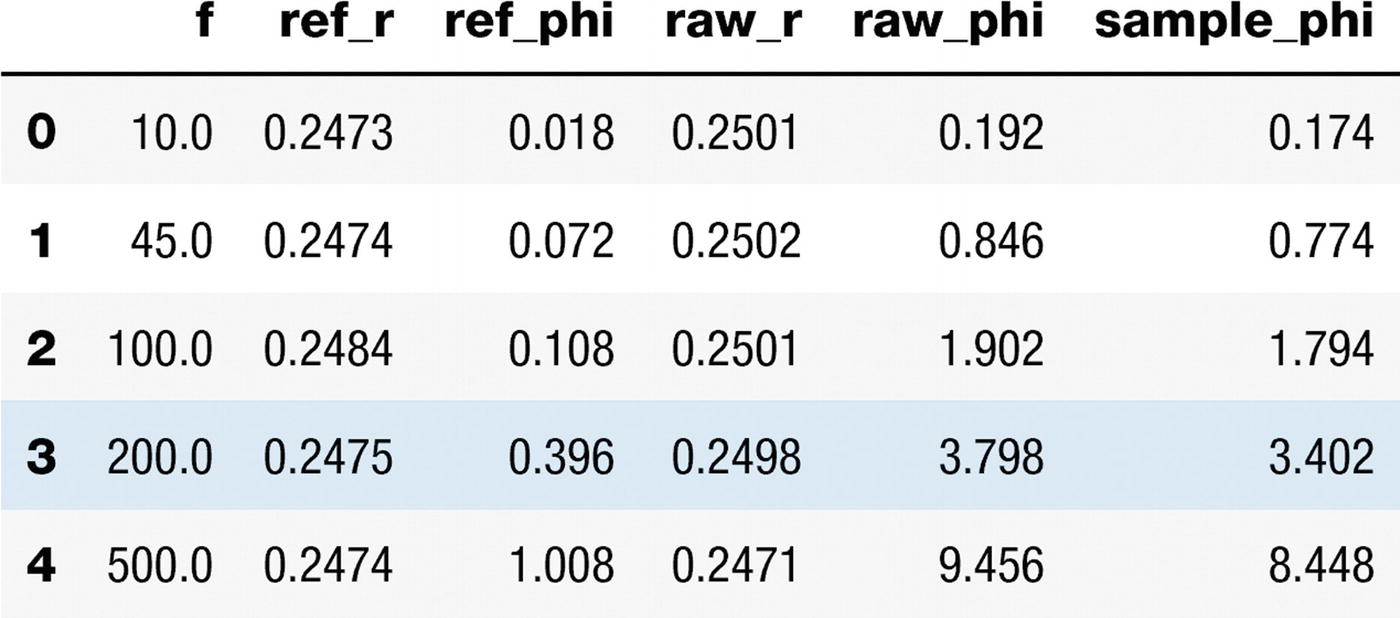
We can check the content of one of the files. Let’s type, for example,
get_df(files[2]).head()
You can see in Figure 9-6 the first five records of the file with index 2.
Figure 9-6
First five records of the file with index 2
The file contains more information than we require.
We have the frequency f, which we must convert to the angular frequency ω (there is a factor 2π between the two), and we must calculate the tangent of θ. We do this with the following code:
adding, in this way, two new columns to each data frame. At this point, we must find a good approximation for f, KSV1, and KSV2, to be able to create our dataset. To give you an example and to make this chapter more concise, let’s consider only one temperature: T = 45∘C. Let’s filter from all our data only that which were measured at this temperature. To do this, we can use the following code:
First, we convert the lists T_list and O2_list to pandas data frames, because, in this format, it is easier to select the right data. Then you may notice that we select all files with T = 45∘C in a data frame files45. Additionally, we select the data frame for T = 45∘C and O2 = 0%, and we call it dfref. The reason is that at the beginning, I gave you a formula for θ that involved tan θ (ω, T, O2 = 0). dfref will contain exactly the measured data for tan θ (ω, T, O2 = 0). Remember that we must model the quantity
I know this is getting complicated, but hold on, we are almost done. Selecting the right data frame from the list of data frames is slightly more complicated but can be done in this way:
from itertools import compress
A = Tdf['T'] == T
data = list(compress(df_list, A))
B = (Tdf['T']==T) & (Odf['O2']==0)
dataref_ = list(compress(df_list, B))
compress is easy to understand. You can find more information on the official documentation page, available at https://goo.gl/xNZEHH. Basically, the idea is that given two lists, d and s, the output of compress(d,s) is given by a new list equal to [(d[0] if s[0]), (d[1] if s[1]), ...]. In our case, A and B are lists made up of Boolean values, so the code returns only the values of df_list for the position in the list A that have True.
Using nonlinear fitting, we will find the values for f, KSV1, and KSV2 for each value of ω we have at our disposal. We must loop over all the values of ω, fit the function
with respect to O2, using the function
def fitfunc(x, f, KSV, KSV2):
return (f/(1.0+KSV*x)+ (1.0-f)/(1+KSV2*x))
to extract f, KSV1, and KSV2 for each O2 value. I did it with this code:
Take some time to study the code. The code is so convoluted because each file contains data at a fixed O2 value. We want to build, for each frequency value, an array containing the values we want to fit as a function of O2. That is why we must do some data wrangling. In the lists f, KSV, and KSV2, we now have the values we found with respect to the frequency. Let’s first select only the values for angular frequencies between 3000 and 100,000.
w_ = w[4:20]
f_ = f[4:20]
KSV_ = KSV[4:20]
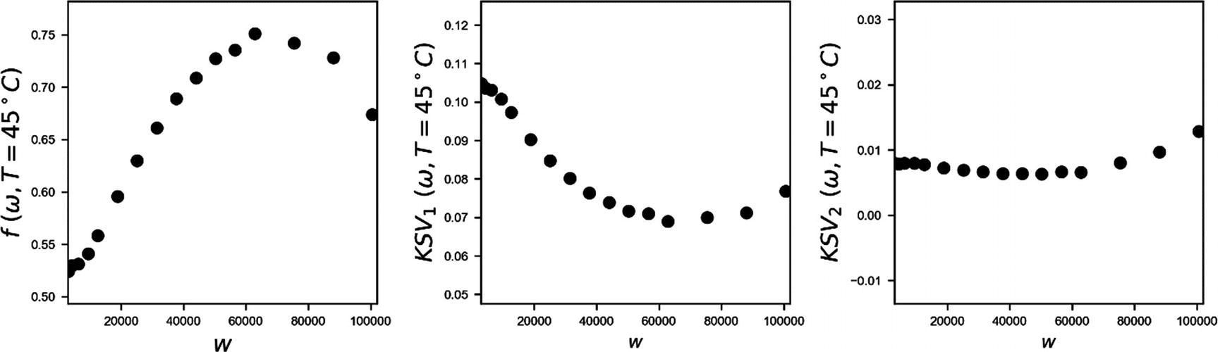
In Figure 9-7, you can see how f, KSV1, and KSV2 depend on the angular frequency.
Figure 9-7
Dependency of f, KSV1, and KSV2 on the angular frequency
There is another small problem we must overcome. We must be able to calculate f, KSV, and KSV2 for any value of ω, not only for the ones we have obtained. To do this, we must use interpolation. To save some time, we will not develop the interpolation functions from scratch. Instead, we will use the interp1d function from the SciPy package.
from scipy.interpolate import interp1d
We will do it in this way:
finter = interp1d(wred, f, kind="cubic")
KSVinter = interp1d(wred, KSV, kind = 'cubic')
KSV2inter = interp1d(wred, KSV2, kind = 'cubic')
Note that finter, KSVinter, and KSV2inter are functions that accept as input a value for ω, as a NumPy array and return the value of f, KSV1, and KSV2, respectively. The continuous line in Figure 9-8 shows the interpolated functions obtained by the points in Figure 9-7.
Figure 9-8
Dependency of f, KSV1, and KSV2 on the angular frequency. The continous line is the interpolated function.
At this point, we have all the ingredients we need. We can finally create our training dataset with the formula
Let’s now create 5000 observations for random values of O2.
X = tf.placeholder(tf.float32, [nx, None]) # Inputs
Y = tf.placeholder(tf.float32, [1, None]) # Labels
# Let's build our network
Z1 = tf.nn.sigmoid(tf.matmul(W1, X) + b1) # n1 x n_dim * n_dim x n_obs = n1 x n_obs
Z2 = tf.nn.sigmoid(tf.matmul(W2, Z1) + b2) # n2 x n1 * n1 * n_obs = n2 x n_obs
Z3 = tf.nn.sigmoid(tf.matmul(W3, Z2) + b3)
Z4 = tf.matmul(W4, Z3) + b4
y_ = Z2
This, at least, is how I began. I chose as output of the network a neuron with an identity activation function y_= Z2. Unfortunately, the training was not working and very unstable. Because I had to predict a percentage, I needed an output between 0 and 100. So, I decided to try a sigmoid activation function multiplied by 100.
y_ = tf.sigmoid(Z2)*100.0
Suddenly, the training worked beautifully. I used the Adam optimizer.
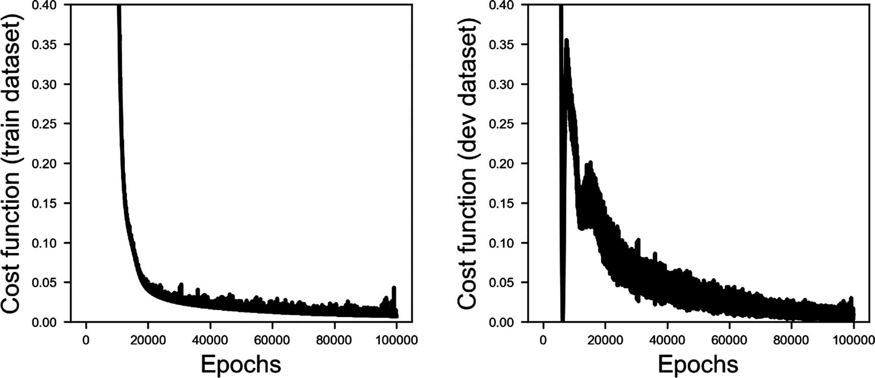
You should understand this code now without too many explanations. It is basically what we have used several times previously. You may have noticed that I have initialized the weights randomly. I tried several strategies, but this seemed to be the one that worked best. It is very instructive to check how the training is going. In Figure 9-10, you can see the cost function evaluated on the training dataset and on the experimental dev dataset. You can see how it oscillates. There are mainly two reasons for this.
The first is that we are using mini-batches, and, therefore, the cost function oscillates
The second reason is that the experimental data is noisy, because the measuring apparatus is not perfect. The gas mixer, for example, has an absolute error of roughly 1–2%, which means that if we have an experimental observation for O2 = 60%, it could be as low as 58% or 59% and as high as 61% or 62%.
Given this error, one should expect to have, on average, an absolute error of ca. 1% in our prediction.
Note
Roughly speaking, the output of a well-trained network will never be able to exceed the accuracy of the target variables used. Remember to always check the errors you may have on your target variables, to estimate how accurate they are. In the preceding example, because our target values for O2 have a maximum absolute error of ±1% (that is, the experimental error), the expected error for the results of the network will be of this order of magnitude.Caution The network will learn the function that produces a certain output, given a specific input. If the output is wrong, the learned function will also be wrong.
Figure 9-10
Cost function vs. the epochs evaluated on the training and on the dev dataset
Finally, let’s check how the network performs.
You should keep in mind that our dev dataset is tiny, making the oscillations even more evident. In Figure 9-11, you can see the predicted value for O2 vs. the measured value. As you can see, they lie beautifully on the diagonal.
Figure 9-11
Predicted value for O2 vs. the measured value
In Figure 9-12, you can see the absolute error calculated on the dev dataset for O2 ∈ [0,100].
Figure 9-12
Absolute error calculated on the dev dataset for O2 ∈ [0,100]
The results are stunningly good. For all values of O2, except for 100%, the error lies below 1%. Remember that our network learned from an artificially created dataset. This network could now be used in this type of sensor without the need of implementing complicated mathematical equations for the estimation of O2. The next phase of this project will be to get automatically ca. 10,000 measurements at various values of the temperature T and the oxygen concentration O2 and use those measurements as a training set to predict both T and O2 at the same time.