In Chapter 2, we did some amazing things with one neuron, but that is hardly flexible enough to tackle more complex cases. The real power of neural networks comes to light when several (thousand, even million) neurons interact with each other to solve a specific problem. The network architecture (how neurons are connected to each other, how they behave, and so on) plays a crucial role in how efficient the learning of a network is, how good its predictions are, and what kind of problems it can solve.
There are many kinds of architectures that have been extensively studied and are very complex, but from a learning perspective, it is important to start from the most simple kind of neural network with multiple neurons. It makes sense to begin with so-called feedforward neural networks, in which data enters at the input layer and passes through the network, layer by layer, until it arrives at the output layer. (This gives the networks their name: feedforward neural networks.) In this chapter, we will consider networks in which each neuron in a layer gets its input from all neurons from the preceding layer and feeds their output into each neuron of the next layer.
As is easy to imagine, with more complexity come more challenges. It is more difficult to achieve fast learning and good accuracy; the number of hyperparameters that are available grows, due to the increased network complexity; and a simple gradient descent algorithm will no longer cut it when dealing with big datasets. When developing models with many neurons, we will need to have at our disposal an expanded set of tools that will allow us to deal with all the challenges that these networks present. In this chapter, we will start to look at some more advanced methods and algorithms that will allow us to work efficiently with big datasets and big networks. These complex networks become good enough to do some interesting multiclass classification, one of the most frequent tasks that big networks are required to perform (for example, handwriting recognition, face recognition, image recognition, and so on), so I have chosen a dataset that will allow us to do some interesting multiclass classification and study its difficulties.
I will start the chapter by discussing the network architecture and the needed matrix formalism. A short overview of the new hyperparameters that come with this new type of network is then given. How to implement multiclass classification using the softmax function , and what kind of output layer is needed, is then explained. Then, before starting with Python code, a brief digression is taken to explain in detail what exactly overfitting is, with a simple example, and how to conduct a basic error analysis with complex networks. Then we will start to use TensorFlow to construct bigger networks, applying them to a MNIST-similar dataset, based on images of clothing items (which will be lots of fun). We will look at how to make the gradient descent algorithm covered in Chapter 2 faster, introducing two new variations: stochastic and mini-batch gradient descent. Then we will look at how to add many layers in an efficient way and how to initialize the weights and the biases in the best way possible, to make training fast and stable. In particular, we will look at Xavier and He initialization for sigmoid and the ReLU activation function, respectively. Finally, a rule of thumb on how to compare complexity of networks going beyond only the number of neurons is offered, and the chapter concludes with some tips on how to choose the right networks.
Network Architecture
 ), several layers (called hidden, because they are sandwiched between the input and the output layers
, so they are “invisible” from the outside, so to speak), and an output layer. In each layer, you may have one to several neurons. The main property of such a network is that each neuron receives input from each neuron in the preceding layer and feeds its output to every neuron in the next layer. In Figure 3-1, you can see a graphical representation of such a network.
), several layers (called hidden, because they are sandwiched between the input and the output layers
, so they are “invisible” from the outside, so to speak), and an output layer. In each layer, you may have one to several neurons. The main property of such a network is that each neuron receives input from each neuron in the preceding layer and feeds its output to every neuron in the next layer. In Figure 3-1, you can see a graphical representation of such a network.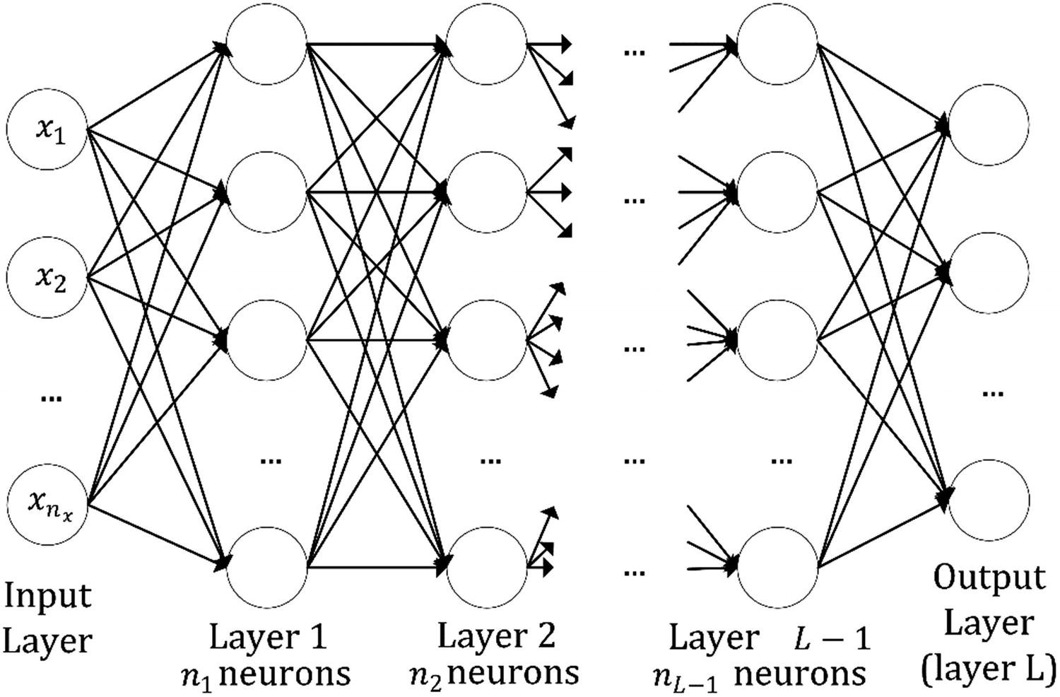
Diagram of a multilayered deep feedforward neural network, in which each neuron receives input from each neuron in the preceding layer and feeds its output to every neuron in the subsequent layer
L: Number of hidden layers, excluding the input layer but including the output layer
nl: Number of neurons in layer l

![$$ {w}_{ikern0.125em j}^{left[l
ight]} $$](http://images-20200215.ebookreading.net/10/2/2/9781484237908/9781484237908__applied-deep-learning__9781484237908__images__463356_1_En_3_Chapter__463356_1_En_3_Chapter_TeX_IEq2.png) . In Figure 3-2, I have drawn only the first two layers (input and layer 1) of our generic network of Figure 3-1, with the weights between the first neuron in the input layer and all the others in layer 1. All other neurons are grayed out for clarity.
. In Figure 3-2, I have drawn only the first two layers (input and layer 1) of our generic network of Figure 3-1, with the weights between the first neuron in the input layer and all the others in layer 1. All other neurons are grayed out for clarity.
The first two layers of a generic neural network , with the weights of the connections between the first neuron in the input layers and the others in the second layer. All other neurons and connections are drawn in light gray, to make the diagram clearer.

This means that our matrix W[1] has dimensions n1 × nx. Of course, this can be generalized between any two layers l and l − 1, meaning that the weight matrix between two adjacent layers l and l − 1, indicated by W[l], will have dimensions nl × nl − 1. By convention, n0 = nx is the number of input features (not the number of observations that we indicate with m).
Note
The weight matrix between two adjacent layers l and l − 1, which we indicate with W[l ], will have dimensions nl × nl − 1, where, by convention, n0 = nx is the number of input features.
The bias (indicated by b in Chapter 2) will be a matrix this time. Remember that each neuron that receives inputs will have its own bias, so when considering our two layers, l and l − 1, we will require nl different values of b. We will indicate this matrix with b[l], and it will have dimensions nl × 1.
Note
The bias matrix for two adjacent layers l and l − 1, which we indicate with b[l], will have dimensions nl × 1.
Output of Neurons
![$$ {widehat{y}}_i^{left[1
ight]} $$](http://images-20200215.ebookreading.net/10/2/2/9781484237908/9781484237908__applied-deep-learning__9781484237908__images__463356_1_En_3_Chapter__463356_1_En_3_Chapter_TeX_IEq3.png) and assume that all neurons in layer l use the same activation function, which we will indicate by g[l]. Then we will have
and assume that all neurons in layer l use the same activation function, which we will indicate by g[l]. Then we will have![$$ {widehat{y}}_i^{left[1
ight]}={g}^{left[1
ight]}left({z}_i^{left[1
ight]}
ight)={g}^{left[i
ight]}kern0.75em left(sum limits_{j=1}^{n_x}left({w}_{ij}^{left[1
ight]} {x}_j+{b}_i^{left[1
ight]}
ight)
ight) $$](http://images-20200215.ebookreading.net/10/2/2/9781484237908/9781484237908__applied-deep-learning__9781484237908__images__463356_1_En_3_Chapter__463356_1_En_3_Chapter_TeX_Equc.png)
![$$ {z}_i^{left[1
ight]}=sum limits_{j=1}^{n_x}left({w}_{ij}^{left[1
ight]} {x}_j+{b}_i^{left[1
ight]}
ight) $$](http://images-20200215.ebookreading.net/10/2/2/9781484237908/9781484237908__applied-deep-learning__9781484237908__images__463356_1_En_3_Chapter__463356_1_En_3_Chapter_TeX_Equd.png)
![$$ {Z}^{left[1
ight]}={W}^{left[1
ight]}X+{b}^{left[1
ight]} $$](http://images-20200215.ebookreading.net/10/2/2/9781484237908/9781484237908__applied-deep-learning__9781484237908__images__463356_1_En_3_Chapter__463356_1_En_3_Chapter_TeX_Eque.png)
where Z[1] will have dimensions n1 × 1, and where with X, we have indicated our matrix with all our observations (rows for the features, and columns for observations), as I have already discussed in Chapter 2. We assume here that all neurons in layer l will use the same activation function that we will indicate with g[l].
![$$ {Z}^{left[l
ight]}={W}^{left[l
ight]}{Z}^{left[l-1
ight]}+{b}^{left[l
ight]} $$](http://images-20200215.ebookreading.net/10/2/2/9781484237908/9781484237908__applied-deep-learning__9781484237908__images__463356_1_En_3_Chapter__463356_1_En_3_Chapter_TeX_Equf.png)
![$$ {Y}^{left[l
ight]}={g}^{left[l
ight]}left({Z}^{left[l
ight]}
ight) $$](http://images-20200215.ebookreading.net/10/2/2/9781484237908/9781484237908__applied-deep-learning__9781484237908__images__463356_1_En_3_Chapter__463356_1_En_3_Chapter_TeX_Equg.png)
where the activation function acts, as usual, element by element.
Summary of Matrix Dimensions
W[l] has dimensions nl × nl − 1 (where we have n0 = nx by definition)
b[l] has dimensions nl × 1
Z[l − 1] has dimensions nl − 1 × 1
Z[l] has dimensions nl × 1
Y[l] has dimensions nl × 1
In each case, l goes from 1 to L.
Example: Equations for a Network with Three Layers

A practical example of a feedforward neural network
![$$ {widehat{Y}}^{left[1
ight]}={g}^{left[1
ight]}left({W}^{left[1
ight]}X+{b}^{left[1
ight]}
ight) $$](http://images-20200215.ebookreading.net/10/2/2/9781484237908/9781484237908__applied-deep-learning__9781484237908__images__463356_1_En_3_Chapter__463356_1_En_3_Chapter_TeX_IEq4.png) , where W[1] has dimensions 3 × nx, b has dimensions 3 × 1, and X has dimensions nx × m
, where W[1] has dimensions 3 × nx, b has dimensions 3 × 1, and X has dimensions nx × m![$$ {widehat{Y}}^{left[2
ight]}={g}^{left[2
ight]}left({W}^{left[2
ight]}{Z}^{left[1
ight]}+{b}^{left[2
ight]}
ight) $$](http://images-20200215.ebookreading.net/10/2/2/9781484237908/9781484237908__applied-deep-learning__9781484237908__images__463356_1_En_3_Chapter__463356_1_En_3_Chapter_TeX_IEq5.png) , where W[2] has dimensions 2 × 3, b has dimensions 2 × 1, and Z[1] has dimensions 3 × m
, where W[2] has dimensions 2 × 3, b has dimensions 2 × 1, and Z[1] has dimensions 3 × m![$$ {widehat{Y}}^{left[3
ight]}={g}^{left[3
ight]}left({W}^{left[3
ight]}{Z}^{left[2
ight]}+{b}^{left[3
ight]}
ight) $$](http://images-20200215.ebookreading.net/10/2/2/9781484237908/9781484237908__applied-deep-learning__9781484237908__images__463356_1_En_3_Chapter__463356_1_En_3_Chapter_TeX_IEq6.png) , where W[3] has dimensions 1 × 2, b has dimensions 1 × 1, and Z[2] has dimensions 2 × m
, where W[3] has dimensions 1 × 2, b has dimensions 1 × 1, and Z[2] has dimensions 2 × m
and your network output, ![$$ {widehat{Y}}^{left[3
ight]} $$](http://images-20200215.ebookreading.net/10/2/2/9781484237908/9781484237908__applied-deep-learning__9781484237908__images__463356_1_En_3_Chapter__463356_1_En_3_Chapter_TeX_IEq7.png) , will have, as expected, dimensions 1 × m.
, will have, as expected, dimensions 1 × m.
All this may seem rather abstract (and, in fact, it is). You will see later in the chapter how easy it is to implement in TensorFlow, simply by building the right computational graph, based on the steps just discussed.
Hyperparameters in Fully Connected Networks
Number of layers: L
Number of neurons in each layer: ni for i from 1 to L
Choice of activation function for each layer: g[l]
Number of iterations (or epochs)
Learning rate
sof tmax Function for Multiclass Classification
You will still have to suffer a bit more theory before getting to some TensorFlow code. The kinds of networks described in this chapter start to be complex enough to be able to perform some multiclass classification with reasonable results. To do this, we must first introduce the softmax function.


So, S(z)i behaves like a probability, because its sum over i is 1, and its elements are all less than 1. We will consider S(z)i as a probability distribution over k possible outcomes. For us, S(z)i will simply be the probability of our input observation of being of class i. Let’s suppose we are trying to classify an observation into three classes. We may get the following output: S(z)1 = 0.1, S(z)2 = 0.6, and S(z)3 = 0.3. That means that our observation has a 10% probability of being of class 1, a 60% probability of being of class 2, and 30% probability of being of class 3. Normally, one chooses to classify the input observation into the class with the higher probability, in this example, class 2, with 60% probability.
Note
We will look at S(z )i as a probability distribution over k with i = 1, …, k possible outcomes. For us, S(z )i will simply be the probability of our input observation being of class i.
To be able to use the softmax function for classification, we will have to use a specific output layer. We will have to use ten neurons, each of which will give zi as its output, and then one neuron that will output S(z). This neuron will have the softmax function as activation function and will have as inputs the 10 outputs, zi, of the last layer with 10 neurons. In TensorFlow, you use the tf.nn.softmax function applied to the last layer with 10 neurons. Remember that this tensorflow function will act element by element. Later in the chapter, you will find a concrete example showing how to implement this from start to finish.
A Brief Digression: Overfitting
One of the most common problems that you will encounter when training deep neural networks will be overfitting. What can happen is that your network may, owing to its flexibility, learn patterns that are due to noise, errors, or simply wrong data. It is very important to understand what overfitting is, so I will give you a practical example of what can happen, to give you an intuitive understanding of it. To make it easier to visualize, I will work with a simple two-dimensional dataset, which I will create for the purpose. I hope that at the end of the next section, you will have a clear idea of what overfitting is.
A Practical Example of Overfitting


where, as usual, m indicates the number of data points we have. I don’t want only to determine all the parameters aj, but also the value of K that best approximates our data. K, in this case, measures our model complexity. For example, for K = 0, we simply have f (x(i)) = a0 (a constant), the simplest polynomial we can think of. For higher K, we have higher order polynomials, meaning that our function is more complex, having more parameters available for training.


To add some random noise to the function, we have used the function np.random.normal(0, 1, size=len(x)), which generates a numpy array of random values from a normal distribution of length len(x), with average 0 and standard deviation 1.

The data we have generated with a = 1, b = 2, and c = 3, as described in the text

The linear model misses the main feature of the data, being too simple. In this case, the model has high bias.

The results for a 2-degree polynomial

The results for a 21-degree polynomial model
Now, this model shows features that we know are wrong, because we created our data. These features are not present, but the model is so flexible that it captures the random variability that we have introduced with noise. Here, I am referring to the oscillations that have appeared using this high-ordered polynomial.

Result of our model, with a 21-degree polynomial fitted to 10 different datasets generated with different random noise values added

Results of our linear model applied to data in which we have randomly changed the random noise. For easier comparison with Figure 3-8, I have used the same scale.
You can see that our model is much more stable. Our linear model does not capture any feature that is dependent on our noise, but it misses the main features of our data (the concave nature). We are talking here of high bias.

Bias and variance
In the case of neural networks, we have many hyperparameters (number of layers, number of neurons in each layer, activation function, and so on), and it is very difficult to know in which regime we are. How can we tell if our model has a high variance or a high bias, for example? I will dedicate an entire chapter to this subject, but the first step in performing this error analysis is to split our dataset into two different ones. Let’s see what this means and why we do it.
Note
The essence of overfitting is to have unknowingly extracted some of the residual variation (i.e., the noise) as if that variation represented the underlying model structure (see Burnham, K. P.; Anderson, D. R., Model Selection and Multimodel Inference, 2nd ed., New York; Springer-Verlag, 2002). The opposite is called underfitting—when the model cannot capture the structure of the data.
The problem with overfitting and deep neural networks is that there is no way of visualizing easily the results, and, therefore, we require a different approach to determine if our model is overfitting, underfitting, or is just right. This can be achieved by splitting our dataset into different parts and evaluating and comparing the metrics on all of them. Let’s explore the basic idea in the next section.
Basic Error Analysis
Training dataset: The model is trained on this dataset, using the inputs and the relative labels, by an optimizer algorithm such as gradient descent, as we did in Chapter 2. Often, this set is called the “train set.”
Development (or validation) set: The trained model will then be used on this dataset, to check how it is doing. On this dataset, we will test different hyperparameters. For example, we can train two different models with a different number of layers on the training dataset and test them on this dataset, to check how they are doing. Often, this set is termed the “dev set.”
Four different cases to show how to recognize overfitting from the training and the dev set error
Error | Case A | Case B | Case C | Case D |
|---|---|---|---|---|
Training set error | 1% | 15% | 14% | 0.3% |
Dev set error | 11% | 16% | 32% | 1.1% |
Case A: Here, we are overfitting (high variance), because we are doing very well on the training set, but our model generalizes very badly to our dev set (refer again to Figure 3-8).
Case B: Here, we see a problem with high bias, meaning that our model is not doing very well generally, on both datasets (refer again to Figure 3-9).
Case C: Here, we have a high bias (the model cannot predict very well the training set) and high variance (the model does not generalize well on the dev set).
Case D: Here, everything seems OK. The error is good on the train set and good on the dev set. That is a good candidate for our best model.
I will explain all these concepts more thoroughly later in the book, where I will provide recipes for how to solve problems of high bias, high variances, both, or even more complex cases.
To recap: To perform a very basic error analysis, you will have to split your dataset into at least two sets: train and dev. You should then calculate your metric on both sets and compare them. You want to have a model that has low error on the train set and on the dev set (as in Case D, in the preceding example), and the two values should be comparable.
Note
Your main takeaways from this section should be (1) a set of recipes and guidelines is required for understanding how your model is doing (is it overfitting, underfitting, or is it just right?); (2) to answer the preceding questions, you must split your dataset in two, to perform the relevant analysis. Later in the book, you will see what you can do with a dataset split into three, or even four, parts.
The Zalando Dataset
Zalando SE is a German e-commerce company based in Berlin. The company maintains a cross-platform store that sells shoes, clothing, and other fashion items.3 For a kaggle competition (if you don’t know what this is, check the website www.kaggle.com , from which you can participate in many competitions that have the goal of solving problems with data science), Zalando prepared a MNIST-similar dataset of images of its clothing, for which they provided 60,000 training images and 10,000 test images. As in MNIST, each image was 28 × 28 pixels in grayscale. Zalando grouped all images in ten different classes and provided the labels for each image. The dataset has 785 columns. The first column is the class label (an integer going from 0 to 9), and the remaining 784 contain the pixel gray value of the image (you can calculate that as 28 × 28 = 784), exactly as we have seen in Chapter 2, in the discussion related to the MNIST dataset of handwritten digits.
0: T-shirt/top
1: Trouser
2: Pullover
3: Dress
4: Coat
5: Sandal
6: Shirt
7: Sneaker
8: Bag
9: Ankle boot

One example from each of the ten classes in the Zalando dataset
The dataset has been provided under the MIT License.4 The data file can be downloaded from kaggle ( www.kaggle.com/zalando-research/fashionmnist/data ) or directly from GitHub ( https://github.com/zalandoresearch/fashion-mnist ). If you choose the second option. you will have to prepare the data a bit. (You can convert it to CSV with the script located at https://pjreddie.com/projects/mnist-in-csv/ .) If you download it from kaggle, the data will already be in the correct format. You will find two CSV files zipped on the kaggle web site. When unzipped, you will have fashion-mnist_train.csv, with 60,000 images (roughly 130MB), and fashion-mnist_test.csv, with 10,000 (roughly 21MB). Let’s fire up a Jupyter notebook and start coding!
You can also read the file with standard NumPy functions (such as loadtxt()), but using read_csv() from pandas gives you a lot of flexibility in slicing and analyzing your data. Additionally, it is a lot faster. Reading the file (that is, roughly 130MB) with pandas takes about 10 seconds, while with NumPy, it takes 1 minute, 20 seconds on my laptop. So, if you are dealing with big datasets, keep this in mind. It is common practice to use pandas to read and prepare the data. If you aren’t familiar with pandas, don’t worry. All you need to understand will be explained in detail.
Note
Remember: You should not focus on the Python implementation. Focus on the model, on the concepts behind the implementation. You can achieve the same results using pandas, NumPy, or even C. Try to concentrate on how to prepare the data, how to normalize it, how to check the training, and so on.

With data_train.head() the command, you can check the first five rows of your dataset
giving the column name in square brackets.
Now the tensor labels have the dimension (1, 60000), as we want.
Labels: This has the dimensions 1 × m (1 × 60000) and contains the class labels (integers from 0 to 9).
Train: This has the dimensions nx × m (784 × 60000) and contains the features, in which each row contains the grayscale value of a single pixel in the image (remember 28 × 28 = 784).
Building a Model with tensorflow
Now it is time to expand what we did with TensorFlow in Chapter 2 with one neuron to networks with many layers and neurons. Let’s first discuss the network architecture and what kind of output layer we need, and then let’s build our model with TensorFlow.
Network Architecture

The network architecture with a single hidden layer. During our analysis, we will vary the number of neurons, n1, in the hidden layer.


We create an output layer with ten neurons. In this way, we will have our ten values as output.
Then we feed the ten values to a new neuron (let’s call it “softmax” neuron) that will take the ten inputs and give as output ten values that are all less than 1 and that add up to 1.

The final neuron in our network that transforms the ten inputs in probabilities

That is exactly what the tensorflow function tf.nn.softmax() does. It takes a tensor as input and returns a tensor with the same dimensions as the input but “normalized,” as discussed previously. In other words, if we feed z = (z1 z2 … z10) to the function, it will return a tensor with the same dimensions as z, meaning 1 × 10, where each element is the last equation.
Modifying Labels for the softmax Function—One-Hot Encoding
where Y contains our labels and y_ is the result of our network. So, the two tensors must have the same dimensions. In our case, I explained to you that our network will give as output a vector with ten elements, while a label in our dataset is simply a scalar. Therefore, we have y_ that has dimensions (10,1) and Y that has dimensions (1,1). This will not work if we don’t do something smart. We must transform our labels in a tensor that has dimensions (10,1). A vector with a value for each class is also required, but what value should we use?
Examples of How One-Hot Encoding Works (Remember that labels go from 0 to 9 as indexes.)
Label | One-Hot Encoded Label |
|---|---|
0 | (1,0,0,0,0,0,0,0,0,0) |
2 | (0,0,1,0,0,0,0,0,0,0) |
5 | (0,0,0,0,0,1,0,0,0,0) |
7 | (0,0,0,0,0,0,0,1,0,0) |

Graphical representation of the process of one-hot encoding a label
First, you create a new array with the right dimensions: (60000,10), then you fill it with zeros with the NumPy function np.zeros((60000,10)). Next, you set to 1 only the columns related to the label itself, using pandas functionalities to slice data frames with the line labels_[np.arange(60000), labels] = 1. Then you transpose it, to have the dimensions we want at the end: (10, 60000), where each column indicates a different observation.
Now in our code, we can finally compare Y and y_, because both now have the dimensions (10,1) for one observation, or when considering the entire training dataset of (10, 60000). Each row in y_ will now represent the probability of our observation as being of a specific class. At the very end, when calculating the accuracy of our model, we will assign the class with the highest probability to each observation.
Note
Our network will give us the ten probabilities for the observation as being of each of the ten classes. At the end, we will assign to the observation the class that has the highest probability.
The tensor flow Model
When we initialize the weights, use the code tf.Variable(tf. truncated_normal ([n1, n_dim], stddev=.1)). The truncated_normal() function will return values from a normal distribution, with the peculiarity that values that are more than 2 standard deviation from the average will be dropped and repicked. The reason for choosing a small stddev of 0.1 is to avoid that the output of the ReLU activation function becomes too big and, therefore, nans start to appear, owing to Python not being able to calculate properly numbers that are too big. I will discuss a better way of choosing the right stddev later in the chapter.
Our last neuron will use the softmax function: y_ = tf.nn.softmax(Z2,0). Remember that y_ will not be a scalar but a tensor of the same dimensions as Z2. The second parameter, 0, tells tensorflow that we want to apply the softmax function along the vertical axis (the rows).
The two parameters n1 and n2 define the number of neurons in the different layers. Remember that the second (output) layer must have ten neurons to be able to use the softmax function. But we will play with the value for n1. Increasing n1 will increase the complexity of the network.
You should immediately notice one thing: it is very slow. Unless you have a very powerful CPU or have installed TensorFlow with GPU support and you have a powerful graphic card, this code will take, on a 2017 laptop, a few hours (from a couple to several, depending on the hardware you have). The problem is that the model, as we coded it, will create a huge matrix for all observations (that is 60,000) and then will modify the weights and bias only after a complete sweep over all observations. This requires quite some resources, memory, and CPU. If that were the only choice we had, we would be doomed. Keep in mind that in the deep-learning world, 60,000 examples of 784 features is not a big dataset at all. So, we must find a way of letting our model learn faster.
The tf.argmax() function returns the index with the largest value across axes of a tensor. You will remember that when I discussed the softmax function, I said that we will assign an observation to the class that has the highest probability (y_ is a tensor with ten values, each containing the probability for the observation of being of each class). So, tf.argmax(y_,0) will give us the most probable class for each observation. tf.argmax(Y,0) will do the same for our labels. Remember that we one-hot encoded our labels, so that, for example, class 2 will now be (0,0,2,0,0,0,0,0,0). Therefore, tf.argmax([0,0,2,0,0,0,0,0,0],0) will return 2 (the index with the highest value, in this case, the only one different than zero).
Don’t get confused by the fact that the file name contains the word test. Sometimes, the dev dataset is called test dataset. Later in the book, when I discuss error analysis, we will use three datasets: train, dev, and test. To remain consistent throughout the book, I prefer to stick with the name dev, so as not to confuse you with different names in different chapters.
A good exercise would be to include this calculation in your model, so that your model() function automatically returns the two values.
Gradient Descent Variations
In Chapter 2, I described the very basic gradient descent algorithm (also called batch gradient descent). This is not the smartest way of finding the cost function minimum. Let’s have a look at the variations that you need to know, and let’s compare how efficient they are, using the Zalando dataset.
Batch Gradient Descent
The gradient descent algorithm described in Chapter 2 calculates the weights and bias variations for each observation but performs the learning (weights and bias update) only after all observations have been evaluated, or, in other words, after a so-called epoch. (Remember that a cycle through the entire dataset is called an epoch.)
Fewer weights and bias updates mean a more stable gradient, which usually results in a more stable convergence.
Usually, this algorithm is implemented in such a way that all the datasets must be in memory, which computationally is quite intensive.
This algorithm is typically very slow for very big datasets.
After 100 epochs, we only reached an accuracy of 16% on our training set!
Stochastic Gradient Descent
The Stochastic6 gradient descent (abbreviated SGD) calculates the gradient of the cost function and then updates weights and biases for each observation in the dataset.
The frequent updates allow an easy check on how the model learning is going. (You don’t have to wait until all the datasets have been considered.)
In a few problems, this algorithm may be faster than batch gradient descent.
The model is intrinsically noisy, and that may allow it to avoid local minima when trying to find the absolute minimum of the cost function.
On large datasets, this method is quite slow, because it is very computationally intensive, owing to the continuous updates.
The fact that the algorithm is noisy can make it hard for it to settle on a minimum for the cost function, and the convergence may not be as stable as expected.
As mentioned, this method can be quite unstable. For example, using a learning rate of 1e-3 will make nan appear before having reached epoch 100. Try to play with the learning rate and see what happens. You require a rather small value for the method to converge nicely. In comparison, with bigger learning rates (as big as 0.05, for example), a method such as batch gradient descent converges without problems. As I mentioned before, the method is quite computationally intensive and for 100 epochs, requires roughly 35 minutes on my laptop. With this variation, after only 100 epochs, we already would have reached an accuracy of 80%. With this variation, learning is, in terms of epochs, very efficient but also very slow.
Mini-Batch Gradient Descent
With this variation of the gradient descent, datasets are split into a certain number of small (from here the term mini is used) groups of observations (called batches), and weights and biases are updated only after each batch has been fed to the model. This is by far the method most commonly used in the field of deep learning.
The model update frequency is higher than with batch gradient descent but lower than SGD. Therefore, allow for a more robust convergence.
This method is computationally much more efficient than batch gradient descent, or SGD, because fewer calculations and resources are needed.
This variation is by far (as we will see later) the fastest of the three.
The use of this variation introduces a new hyperparameter that must be tuned: the batch size (number of observations in the mini-batch).
In this case, we have used a learning rate of 1e-3—much bigger than the one in SGD—and reached a cost function value of 0.14—a bigger value than the 0.094 reached with SGD but much smaller than the 0.32 value reached with batch gradient descent—and it requires only 2.5 minutes. So, with a factor of 14, it is faster than SGD. After 100 epochs, we achieved an accuracy of 66%.
Comparison of the Variations
Summary of the Findings for Three Variations of Gradient Descent for 100 Epochs
Gradient Descent Variation | Running Time | Final Value of Cost Function | Accuracy |
|---|---|---|---|
Batch gradient descent | 2.5 min | 0.323 | 16% |
Mini-batch gradient descent | 2.5 min | 0.14 | 66% |
Stochastic gradient descent (SGD) | 35 min | 0.094 | 80% |
Now you can see that SGD is the algorithm that achieves the lowest value of cost function with the same number of epochs, although it is by far the slowest. For the mini-batch gradient descent to reach a value of 0.094 for the cost function, it takes 450 epochs and roughly 11 minutes. Still, this is a huge improvement over SGD—31% of the time for the same results.

Comparison of the speed of convergence of a mini-batch gradient descent algorithm with different mini-batch sizes
Note
The best compromise between running time and convergence speed (with respect to number of epochs) is achieved by mini-batch gradient descent. The optimal size of the mini-batches is dependent on your problem, but, usually, small numbers, such as 30 or 50, are a good option. You will find a compromise between running time and convergence speed.
Plot for the Zalando dataset, showing the value of the cost function after 100 epochs vs. the running time required to run through 100 epochs
minibatch_size: The number of observations we want in each batch. Note that if we choose for this hyperparameter a number q that is not a divisor of m (number of observations), or, in other words, m/q is not an integer, we will have the last mini-batch with a different number of observations than all the others. But this will not be an issue for the training. For example, suppose we have a hypothetical dataset with m=100, and you decide to use mini-batch sizes of 32 observations. Then, with m=100, you will have 3complete mini-batches with 32 observations and 1 with just 4, since 100 = 3*32+4. Now you may wonder what will happen with a line such as
X_train_mini = features[:,i:i + 32]
when i=96 and features has only 100 elements. Are we not going over the limits of the array? Fortunately, Python is nice to programmers and takes care of this. Consider the following code:
l = np.arange(0,100)
for i in range (0, 100, 32):
print (l[i:i+32])
The result is
[ 0 1 2 3 4 5 6 7 8 9 10 11 12 13 14 15 16 17 18 19 20 21 22 23 24 25 26 27 28 29 30 31]
[32 33 34 35 36 37 38 39 40 41 42 43 44 45 46 47 48 49 50 51 52 53 54 55 56 57 58 59 60 61 62 63]
[64 65 66 67 68 69 70 71 72 73 74 75 76 77 78 79 80 81 82 83 84 85 86 87 88 89 90 91 92 93 94 95]
[96 97 98 99]
And as you see, the last batch has only four elements, and we don’t get any error. So, you should not worry about this, and you can choose any mini-batch size that works better for your problem.
training_epochs: The number of epochs we want
features: The tensor that contains our features
classes: The tensor that contains our labels
logging_step: This tells the function to print the value of the cost function every logging_step epoch
learning_r: The learning rate we want to use
Note
Writing a function with the hyperparameters as inputs is common practice. This allows you to test different models with different values for the hyperparameters and check which one is better.
Examples of Wrong Predictions

Example of wrongly classified images for each class
Some errors are understandable, such as, for example, that at the lower left of the figure. A shirt has been wrongly classified as a coat. It is also difficult to determine which item is which, and I could easily have made the same mistake. The wrongly classified bag is, on the other hand, easy for a human to sort out.
Weight Initialization
But why choose a standard deviation of 0.1?
![$$ {z}_i=sum limits_{j=1}^{n_x}left({w}_{ij}^{left[1
ight]} {x}_j+{b}_i^{left[1
ight]}
ight) $$](http://images-20200215.ebookreading.net/10/2/2/9781484237908/9781484237908__applied-deep-learning__9781484237908__images__463356_1_En_3_Chapter__463356_1_En_3_Chapter_TeX_Equq.png)
Normally in a deep network, the number of weights is quite big, so you can easily imagine that if the ![$$ {w}_{ikern0.125em j}^{left[1
ight]} $$](http://images-20200215.ebookreading.net/10/2/2/9781484237908/9781484237908__applied-deep-learning__9781484237908__images__463356_1_En_3_Chapter__463356_1_En_3_Chapter_TeX_IEq8.png) are big, the quantity zi, too, can be quite big, and the ReLU activation function can return a nan value, because the argument is too big for Python to calculate it properly. So, you want the zi to be small enough to avoid an explosion of the output of the neurons and big enough to prevent the outputs from dying out and, therefore, making the convergence a very slow process.
are big, the quantity zi, too, can be quite big, and the ReLU activation function can return a nan value, because the argument is too big for Python to calculate it properly. So, you want the zi to be small enough to avoid an explosion of the output of the neurons and big enough to prevent the outputs from dying out and, therefore, making the convergence a very slow process.
Different Initialization Strategies, Depending on Activation Functions
Activation Function | Standard Deviation σ for a Given Layer |
|---|---|
Sigmoid |
|
ReLU |
|


Using this initialization can speed up training considerably and is the standard way in which many libraries initialize weights (for example, the Caffe library).
Adding Many Layers Efficiently
First, we get the dimension of the inputs, to be able to define the right weight matrix.
Then, we initialize the weights with the He initialization discussed in the previous section.
Next, we create the weights W and bias b.
Then, we evaluate the quantity Z and return the activation function evaluated on Z. (Note that in Python, you can pass functions as parameters to other functions. In this case, activation may be tf.nn.relu.)
Now the code is much easier to understand, and you can use it to create networks as big as you wish.
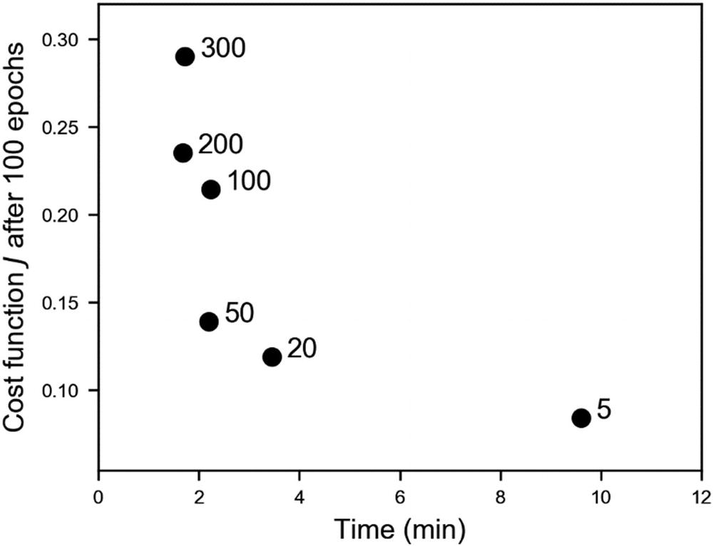
One layer and ten neurons each layer
Two layers and ten neurons each layer
Three layers and ten neurons each layer
Four layers and ten neurons each layer
4 layers and 100 neurons each layer
The cost function vs. epochs for five models, as described in the legend
In case you are wondering , the model with four layers, each with 100 neurons, which seems much better than the others, is starting to go in the overfitting regime, with a train set accuracy of 94% and of 88% on the dev set (after only 200 epochs).
Advantages of Additional Hidden Layers
I suggest you play with the models. Try varying the number of layers, number of neurons, how to initialize the weights, and so on. If you invest some time, you can achieve an accuracy of more than 90% in a few minutes of running time, but that requires some work. If you try several models, you may realize that in this case, using several layers does not seem to accrue benefits vs. a network with just one. This is often the case.
Theoretically speaking, a one-layer network can approximate every function you can imagine, but the number of neurons needed may be very large, and, therefore, the model becomes much less useful. The catch is that the ability to approximate a function does not mean that the network is able to learn to do it, owing, for example, to the sheer number of neurons involved or the time required.
Empirically, it has been shown that networks with more layers require much smaller numbers of neurons to reach the same results and usually generalize better to unknown data.
Note
Theoretically speaking, you don’t need to have multiple layers in your networks, but often, in practice, you should. It is almost always a good idea to try a network of several layers with a few neurons in each, instead of a network with one layer populated by a huge number of neurons. There is no fixed rule on how to decide how many neurons or layers are best. You should try starting with low numbers of layers and neurons and then increase these until your results stop improving.
In addition, having more layers may allow your network to learn different aspects of your inputs. For example, one layer may learn to recognize vertical edges of an image, and another, horizontal ones. Remember that in this chapter, I have discussed networks in which each layer is identical (up to the number of neurons) to all the others. You will see later, in Chapter 4, how you can build networks in which each layer performs very different tasks and is also structured very differently from another, making this kind of network much more powerful for certain tasks that have been discussed previously in this chapter.
You may remember that in Chapter 2, we tried to predict the selling prices of houses in the Boston area. In that case, a network with several layers might reveal more information about how the features relate to the price. For example, the first layer might reveal basic relationships, such as bigger houses equal higher prices. But the second layer might reveal more complex relationships, such as big houses with a smaller numbers of bathrooms equal low selling prices.
Comparing Different Networks

Cost function decrease vs. epochs for a neural network of one hidden layer with, respectively, 1, 5, 15, and 30 neurons, as indicated in the legend. The calculations have been performed with mini-batch gradient descent, with a batch size of 50 and a learning rate of 0.05.
![$$ {Q}^{left[l
ight]}={n}_l{n}_{l-1}+{n}_l={n}_lleft({n}_{l-1}+1
ight) $$](http://images-20200215.ebookreading.net/10/2/2/9781484237908/9781484237908__applied-deep-learning__9781484237908__images__463356_1_En_3_Chapter__463356_1_En_3_Chapter_TeX_Equx.png)

A comparison of the values of Q for different network architectures
Network Architecture | Parameter Q (Number of learnable parameters) | Number of Neurons |
|---|---|---|
Network A: 784 features, 2 layers: n1 = 15, n2 = 10 | QA = 15(784 + 1) + 10 ∗ (15 + 1) = 11935 | 25 |
Network B: 784 features, 16 layers: n1 = n2 = … = n15 = 1, n16 = 10 | QB = 1 ∗ (784 + 1) + 1 ∗ (1 + 1) + … + 10 ∗ (1 + 1) = 923 | 25 |
Network C: 784 features, 3 layers: n1 = 10, n2 = 10, n3 = 10 | QC = 10 ∗ (784 + 1) + 10 ∗ (10 + 1) + 10 ∗ (10 + 1) = 8070 | 30 |
I would like to draw your attention to networks A and B. Both have 25 neurons, but the parameter QA is much bigger (more than a factor of ten) than QB. You can easily imagine how network A will be much more flexible in learning than network B, even if the number of neurons is the same.
Note
I would be misleading you if I told you that this number Q is a measure of how complex or how good a network is. This is not the case, and it may well happen that of all the neurons, only a few will play a role. Therefore, calculating only as I told you will not tell the entire story. There is a vast amount of research on the so-called effective degrees of freedom of deep neural networks, but that goes way beyond the scope of this book. Nonetheless, this parameter will provide a good rule of thumb in deciding if the set of models you want to test are in a reasonable complexity progression.
A comparison of the values of Q for different network architectures
Network Architecture | Parameter Q | Number of Neurons |
|---|---|---|
784 features, 1 layer with 1 neuron, 1 layer with 10 neurons | Q = 1 ∗ (784 + 1) + 10 ∗ (1 + 1) = 895 | 11 |
784 features, 1 layer with 5 neuron, 1 layer with 10 neurons | Q = 5 ∗ (784 + 1) + 10 ∗ (5 + 1) = 3985 | 15 |
784 features, 1 layer with 15 neuron, 1 layer with 10 neurons | Q = 15 ∗ (784 + 1) + 10 ∗ (15 + 1) = 11935 | 25 |
784 features, 1 layer with 30 neuron, 1 layer with 10 neurons | Q = 30 ∗ (784 + 1) + 10 ∗ (30 + 1) = 23860 | 40 |


You should be able to solve a quadratic equation, so I will only give the solution here (hint: try to solve it). This equation is solved for a value of nB = 14.4, but because we cannot have 14.4 neurons, we will have to use the closest integer, which would be nB = 14. For nB = 14, we will have QB = 11560, a value very close to 11935.
Note
Please let me say it again. The fact that the two networks have the same number of learnable parameters does not mean that they can reach the same accuracy. It does not even mean that if one learns very fast the second will learn at all!
Our model with 3 layers with each 14 neurons could, however, be a good starting point for further testing.
Let’s discuss another point that is important when dealing with a complex dataset. Consider our first layer. Suppose we consider the Zalando dataset and we create a network with two layers: the first with one neuron and the second with many. All the complex features that your dataset has may well be lost in your single first neuron, because it will combine all features in one single value and pass the same exact value to all other neurons of the second layer.
Tips for Choosing the Right Network
I hear you crying, “You’ve discussed a lot of cases, given us a lot of formulas, but how can we decide how to design our network?”
When considering a set of models (or network architectures) that you want to test, a good rule of thumb is to start with the less complex one and move to more complex ones. Another is to estimate the relative complexity (to make sure that you are moving in the right direction) of the use of the parameter Q.
In case you cannot achieve good accuracy, check if any of your layers has a particularly low number of neurons. This layer may kill the effective capacity of learning from a complex dataset of your network. Consider, for example, the case with one neuron in Figure 3-20. The model cannot reach low values for the cost function because the network is too simple to learn from a dataset as complex as the Zalando one.
Remember that a low or high number of neurons is always relative to the number of features you have. If you have only two features in your dataset, one neuron may well be sufficient, but if you have few hundred (like in the Zalando dataset where nx = 784), you should not expect one neuron to be enough.
Which architecture you need is also dependent on what you want to do. It is always worth checking online literature to see what others have already discovered about specific problems. For example, it is well known that for image recognition, convolutional networks are very good, so they would be an excellent choice.
Note
When moving from a model with L layers to one with L + 1 layers, it is always a good idea to start with the new model, using a slightly lower number of neurons in each layer, and then increasing them step by step. Remember that more layers have a chance of learning complex features more effectively, so if you are lucky, fewer neurons may be enough. It is something worth trying. Always keep track of your optimizing metric (remember this from Chapter 2?) for all your models. When you are no longer getting much improvement, it may be worth trying completely different architectures (maybe convolutional neuronal networks, etc.).