Microbursts Visualized

Let’s look at what a microburst looks like from a traffic usage pattern. Traditionally network interfaces are monitored using Simple Network Management Protocol (SNMP) tools such as Solarwinds, MRTG, HP OpenView, or the like. These tools usually poll once every five minutes, though some environments poll more often. Polling more often gives more refined graphs due to having more granular data at the cost of increased SNMP traffic on the network. Figure 23-1 depicts a typical interface utilization graph.

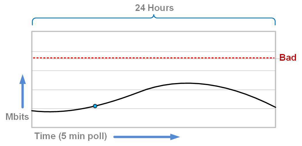
Figure 23-1. Typical interface utilization graph with five-minute SNMP polling

If someone were to come to me and say that the network sucks, I would probably look at the graph and say, “Nope!” The graphs are all below the line that says bad, so go away and bother someone else. The problem is that the graph is not as accurate as we’d like to believe.

The tools producing these graphs do so by polling the devices using something called an SNMP GET. A typical request might be “get the number of bytes that have output from this interface.” This GET will return an integer that is literally the number of bytes that have been sent out the interface since the switch was last booted. And yes, this can be a ridiculously large number. You can see these numbers using the show interface [int-name] counters command. Here’s an example:

Arista-2#sho int e48 counters outgoing
Port       OutOctets    OutUcastPkts    OutMcastPkts    OutBcastPkts
Et48    139617360586        92095180            5451               0

Assuming the default interval, the graphs are created by polling (doing an SNMP get) every five minutes. The latest value is subtracted from the value from the last poll, and that number is put into the graph. It’s literally that simple (our graph is showing Mbits, so some additional math is performed). Let’s see how that would shake out using the counters after five minutes of traffic on this interface:

Arista-2#sho int e48 counters outgoing
Port         OutOctets    OutUcastPkts    OutMcastPkts    OutBcastPkts
Et48      144502369406        95317527            5461               0

Having grabbed the data twice, if we subtract the two OutOctet numbers, we get the number of octets (bytes) sent out by that interface over that interval of time. Let’s use Bash’s expr command to do the math:

Arista-2#bash expr 144502369406 - 139617360586
4885008820

Adding some commas (sorry, Europeans) for formatting, we get the more human readable 4,885,008,820 so 4.8 GigaBYTEs (remember, we measured how many octets were output from this interface over five minutes). If we do some more math, convert that to bits

Arista-2#bash expr 4885008820 * 8
39080070560

and then divide that by the number of seconds in five minutes (300), we get the following:

Arista-2#bash expr 39080070560 / 300
130266901

Adding commas, we get 130,266,901, which is 130.26 Mbps. For the five-minute period between the two SNMP gets, the switch output 130.25 Mbps.

But did it, really?

The problem with this method is granularity. We’ve basically reduced the entire five-minute period to two values and subtracted them to put a number into a graph, but the network did not send a steady state of 130.25 Mbps traffic during those five minutes, and depending on the nature of the traffic on the network, those SNMP graphs that we’ve all been trusting for decades might be misleading us.

In Figure 23-1, you’ll notice a small circle on the graph. At that point in time, I was able to monitor the outbound interface every 1/1,000 of a second. With millisecond accuracy, I collected what the traffic looked like and put it into the graph shown in Figure 23-2.

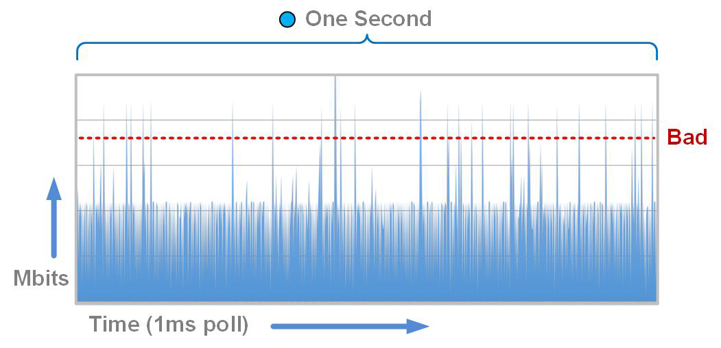
Figure 23-2. Spot from previous graph zoomed in to impossible one-second interval

Holy moly! See those spikes that are crossing the bad line? Those are microbursts, and they’re causing people to think that the network sucks even though the SNMP graphs all look good. Believe it or not, this example doesn’t even scratch the surface of how bad it can be! There can be flat-out buffer-full oversubscription on the interface for short durations that cause packets to be dropped while not even showing up as a blip on the SNMP graphs.

After living through this a couple of times, you learn to sort of smell when it’s happening, but having lived through microburst events that caused performance problems, I can tell you that I would have given my right arm for useful tools that would give me graphs like the 1-second example shown earlier. OK, maybe not my entire right arm, but believe me when I say that the lack of visibility into these buffers is extremely frustrating. I’ve been through enough of these problems that I swear I can smell them, but being unable to prove them makes it difficult to coax management to spend money to fix them. If only someone would make a switch that had real troubleshooting tools at the interface buffer level! Enter LANZ.

Latency analyzer (LANZ) is Arista’s solution to this problem. On certain Arista switches, the Application-Specific Integrated Circuits (ASICs) allow visibility into the interface buffers at a heretofore unheard-of reporting granularity of less than one millisecond. For those of you who can’t keep the whole micro/nano/pico thing straight, a millisecond is one-thousandth of a second.

That’s right, we can now get reports that show the status of our interface buffers 1,000 times per second. Cool, huh? Sounds like too much information to me, but I’m a cranky old nerd. Let’s take a look and see how it works.

Queue Thresholds

To understand what LANZ is doing I’d like to take a brief detour into simple buffer theory. If you’re not familiar with this sort of thing, you’ve probably seen it before when you configure a serial port (such as a console) using the settings for flow control. One of those settings is called XON/XOFF, which I use for this example, but the principles are fundamentally the same regardless of whether it’s RTS/CTS, TCP Source Quench, or Ethernet flow control, though the actual mechanism or configuration might be different. Let’s consider a serial port buffer such as the one shown in Figure 23-3.

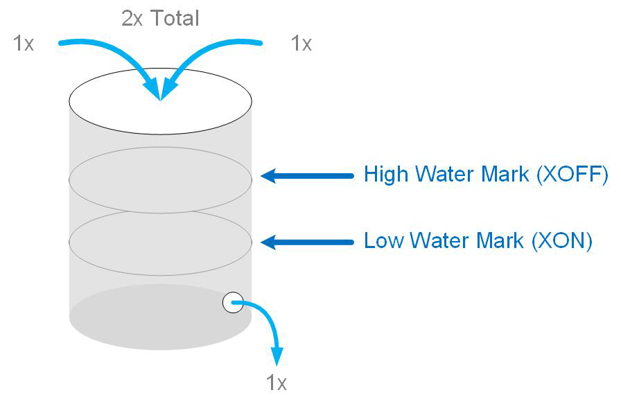
Figure 23-3. Simple serial port buffer

The buffer is shown as a simplistic container, like a 55-gallon drum or a smaller flask. Essentially, 1x worth of water can exit the bottom, but we can easily fill the container with 2x (or more) water. If we continue doing so, the buffer will overflow and water will get all over the floor, and who wants to clean that up? Not me.

To prevent the buffer from overflowing, sensors are installed, and when the water in the container reaches the High-Water Mark, a signal is sent to the people filling the container, telling them to knock it off. This is the XOFF signal in serial flow control. After the inflow of water stops, the container continues to drain at 1x through the bottom. When the water level lowers to the Low-Water Mark, another signal is sent (this time an XON) to people with the hoses who then begin filling the container again. By letting these sensors inform the people filling the container, the container should never overflow. Again, this is the idea behind most flow-control mechanisms out there.

LANZ is not a flow-control mechanism. LANZ is a reporting tool that allows us to see what’s happening within a buffer, but it’s important to understand that LANZ does not affect the flow of data through that buffer. The way that it reports on buffer status is conceptually similar, though, so consider Figure 23-4.

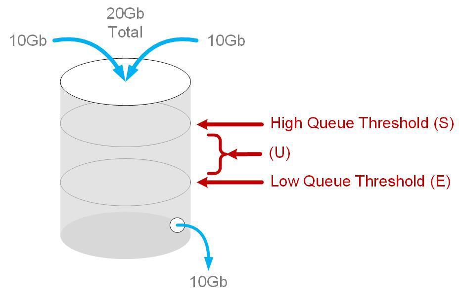
Figure 23-4. LANZ with high- and low-queue thresholds

Here, the container is the buffer for a 10 Gbps Ethernet interface. That buffer can be filled with multiple source interfaces, and if we allow two 10 Gbps Ethernet interfaces to fill the buffer, it will overflow. When the buffer overflows, packets are dropped, and even though there are no mops involved, I’m still the guy who has to clean it up.

With LANZ we configure a High-Queue Threshold, which is similar in principle to the High-Water Mark except that it does not affect flow. It is the threshold at which, when the buffer fills to that point, LANZ will send a Start (S) record. Hopefully, either through some flow-control mechanism or through organic change, the buffer will begin to deplete, during which time LANZ will send Update (U) records. When the Low-Queue Threshold is met, LANZ will send an End (E) record. Some switches, like the 7280R, will send Polling (P) records as well when in polling mode.

Polling mode is the default state on some Arista switches and differs from notification mode in that notification mode uses more hardware resources (which is why it’s not the default on those boxes). Internally there a bunch of different ways that LANZ uses the hardware, which is far beyond the scope of this book. Just know that if you’re seeing only P records that your switch is in polling mode.

For my first example, I have a very simple network setup, as presented in Figure 23-5. This network comprises an Arista 7280R switch hooked up to another Arista 7280R switch. In the first edition of Arista Warrior, I used a Cisco 3750 as the other switch, which caused all sorts of mayhem due to that switch using processed switching for packets destined to the switch. Although amusing, I decided that it was time to embrace the future. Also, back then I had only one old Arista switch to play with, and now I have access to rooms full of them.

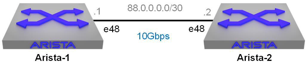
Figure 23-5. A simple LANZ test lab

I’ve connected these two switches using 10 Gbps Twinax cables. Here are the configurations for the two switches to accomplish this simple design. First, Arista-1:

Arista-1(config-if-Et48)#sho run int e48
interface Ethernet48
   description desc [ Arista-2 ]
   no switchport
   ip address 88.0.0.1/30

And now Arista-2:

Arista-2#sho run int e48
interface Ethernet48
   description [ Arista-1 ]
   no switchport
   ip address 88.0.0.2/30

With Arista switches being so damn powerful, there’s no way I could overwhelm that 10 Gbps link with simple pings. There are some additional limitations with the way that LANZ works on the modern 7280Rs with their Jericho ASICs versus the way the older switches worked, so I needed a more interesting solution. I had toyed around with disabling Spanning Tree and making loops with multiple interfaces, but that was too complicated for various reasons. Arista trainer Rich Parkin thought up a cool scenario that allows us to deliver a 10 Gbps amount of traffic easily while lowering the effective speed of one of the interfaces in order to trigger buffering that we can see with LANZ. Figure 23-6 shows that design.

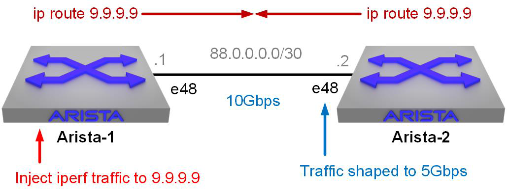
Figure 23-6. A simple LANZ test lab with routing loop

Simply put, we’re going to make a routing loop between the two switches to a destination IP address 9.9.9.9. We’re then going to use traffic-shaping to make the e48 interface on Arista-2 behave like a 5 Gbps interface. We’ll use iperf (more on that in a minute) to inject traffic destined for 9.9.9.9 and then sit back and watch while the mayhem ensues.

Here is the configuration needed to set up the lab with these new requirements:

Arista-1 is simple:

Arista-1#sho run | grep rout  
ip route 9.9.9.9/32 88.0.0.2
ip routing

Arista-2 has a little bit more to it, but first, here are the matching routing commands:

Arista-2(config)#sho run | grep rout
ip route 9.9.9.9/32 88.0.0.1
ip routing

That accomplishes the routing loop, but we need to configure e48 with some additional values in order to throttle the traffic:

Arista-2(config)#sho run int e48
interface Ethernet48
   description [ Arista-1 ]
   load-interval 1
   no switchport
   ip address 88.0.0.2/30
   shape rate 5000000

The load-interval command has no effect on traffic flow and is just there for ease of reporting. The real magic here is the shape rate 5000000 command, which effectively makes the interface behave as if it were only a 5 Gbps port. Although the internals can be a tad more complicated than that, the result is that with 10 Gbps of traffic trying to be sent back to Arista-1, the traffic will need to be buffered, which is what we want to see with LANZ.

With the basic network configured, let’s go in and configure LANZ. We’re only going to do on Arista-2 because that’s where the buffering is set to happen. First, we need to enable the feature globally. We do this by using the queue-monitor length command:

Arista-2#queue-monitor length

At this point, LANZ is running and will record information when the proper thresholds are met. Next, we configure LANZ on the interface connected to the other switch. This is done with a similar command that needs to include two threshold values, the lower threshold and the upper threshold:

Arista-2(config)#int e48
Arista-2(config-if-Et48)#queue-monitor length thresholds 40962 10241

Where did I get those numbers from? Well, they’re the High-Queue threshold and the Low-Queue threshold for the interfaces and are the lowest allowable values on this platform:

Arista-2(config-if-Et48)#queue-monitor length thresholds ?
  <40962-524288000>  high threshold in units of bytes

Arista-2(config-if-Et48)#queue-monitor length thresholds 40962 ?
  <10241-524288000>  low threshold in units of bytes

Arista-2(config-if-Et48)#queue-monitor length thresholds 40962 10241

On the older boxes with different ASICs, like the 7150s, the thresholds were set using buffer segments instead of bytes, and you could configure much lower numbers like this:

Arista-7150(config-if-Et5)#queue-monitor length thresholds 2 1

The 7280s also allow just a High-Queue threshold to be set, so be careful if you’re used to using autocompletion because the word threshold (singular) is what you’ll end up with and you won’t be able to put in the Low-Queue threshold.

With LANZ configured you can check the status with the show queue-monitor length status command:

Arista-2(config-if-Et48)#sho queue-monitor length status
queue-monitor length enabled
queue-monitor length packet sampling is disabled
queue-monitor length update interval in micro seconds:  5000000
Per-Interface Queue Length Monitoring
-------------------------------------
Queue length monitoring is enabled
Queue length monitoring mode is:
   FixedSystem    polling
Maximum queue length in bytes : 524288000
Port thresholds in bytes:
Port     High threshold  Low threshold       Warnings
Cpu               65536          32768
Et1             5242880        2621440
Et2             5242880        2621440
Et3             5242880        2621440
Et4             5242880        2621440
[--output removed--]
Et46            5242880        2621440
Et47            5242880        2621440
Et48              40962          10241
Et49/1          5242880        2621440
Et49/2          5242880        2621440
Et49/3          5242880        2621440
[--output removed--]
Et54/1          5242880        2621440
Et54/2          5242880        2621440
Et54/3          5242880        2621440
Et54/4          5242880        2621440

With this command, we can see a bunch of information about LANZ including the queue thresholds. We can see that we’ve altered the values on e48 from the defaults. We can also see that this switch is configured for polling mode, but we’re going to leave it there for now. Enough configuration; let’s abuse some buffers!

In the first edition of Arista Warrior, I had to resort to sending ping packets from Bash to the remote switch like this:

Arista-1#bash

Arista Networks EOS shell

[admin@Arista-1 ~]$ ping -s 15000 -c 1000 88.0.0.2 > /dev/null &
[1] 9054
[admin@Arista-1 ~]$ ping -s 15000 -c 1000 88.0.0.2 > /dev/null &
[2] 9057
[admin@Arista-1 ~]$ ping -s 15000 -c 1000 88.0.0.2 > /dev/null &
[3] 9060

That certainly works, but it’s lame because with today’s EOS, the iperf tool is installed by default! With the interfaces configured, LANZ turned on, and our routing loop ready to go, let’s get crazy and send a 1 Gb barrage of data into the loop. We’ll do this using iperf from Bash on Arista-1. This command will attempt to send 1 Gbps of traffic using User Datagram Protocol (UDP) to 9.9.9.9:

[admin@Arista-1 ~]$  iperf -uc 9.9.9.9 -b 1G  
------------------------------------------------------------
Client connecting to 9.9.9.9, UDP port 5001
Sending 1470 byte datagrams
UDP buffer size:  208 KByte (default)
------------------------------------------------------------
[  3] local 88.0.0.1 port 54631 connected with 9.9.9.9 port 5001
[ ID] Interval       Transfer     Bandwidth
[  3]  0.0-10.0 sec   968 MBytes   812 Mbits/sec
[  3] Sent 690431 datagrams
[  3] WARNING: did not receive ack of last datagram after 10 tries.

Within a couple of seconds, the interface on Arista-2 is sending at its maximum shape-rate:

Arista-2#sho int e48 | grep rate
  1 second input rate 5.69 Gbps (57.7% with framing overhead), 469536 pkts/sec
  1 second output rate 4.87 Gbps (49.3% with framing overhead), 401408 pkts/sec

Because the routing loop is self-limiting due to Time to Live (TTL), after a few seconds the interface drops back down to zero:

Arista-2#sho int e48 | grep rate
  1 second input rate 0 bps (0.0% with framing overhead), 0 packets/sec
  1 second output rate 0 bps (0.0% with framing overhead), 0 packets/sec

Let’s see what LANZ saw during this assault:

Arista-2#sho queue-monitor length e48

Report generated at 2019-01-16 23:00:59
S-Start, U-Update, E-End, P-Polling, TC-Traffic Class
* Max queue length during period of congestion
Type Time              Intf(TC) Queue     Duration  Ingress                  
                                Length              Port-set                  
                                (bytes)   (usecs)                            
---- ----------------- -------- --------- --------- -----------------------------
P    0:02:38.31162 ago Et48(1)  38936576  12012760  Et1-8,17-20,29-32,41-48,51/1,

Note that some of the rightmost output has been truncated because it’s just too much to fit and I didn’t want it to wrap. The reason for that odd output is sort of interesting, though, so let’s look at that last column, which is the Ingress Port-set. That’s a very strange interface range that I absolutely did not configure. After talking to the developers at Arista, I finally understood what this represented, which is all of the interfaces that are on the same ASIC core as the interface in question. Um…what?

On the Jericho-based switches like the 7280R I’m using here, the ASIC comprises multiple cores just like the cores you’d find in your PC’s CPU. The front-panel interfaces are distributed across multiple cores in the ASIC, and this is reporting the other interfaces found on that core. Another way that you can see this is by using the show platform command. I’m going to do some Linux wizardry here to show you a vastly simplified output. If you’d like to see the entire output, use the show platform jericho mapping command on your 7280R or other Jericho-based Arista switch:

 [admin@Arista-2 ~]$ Cli -p 15 -c "show platform jericho mapping" |
 { head -n3 ; grep Ether; } | awk '{printf "%-12s %s
", $1, $4}'

Jericho0  
Port         Core
Ethernet1    0
Ethernet2    0
Ethernet3    0
Ethernet4    0
Ethernet5    0
Ethernet6    0
Ethernet7    0
Ethernet8    0
Ethernet9    1
Ethernet10   1
Ethernet11   1
Ethernet12   1
Ethernet13   1
Ethernet14   1
Ethernet15   1
Ethernet16   1
Ethernet17   0
Ethernet18   0
Ethernet19   0
Ethernet20   0
[-- output truncated --]

If that huge statement hurts your head, here’s what it’s doing:

1. Issue the CLI command show platform jerich mapping

2. Include the first three lines of the header

3. Include only lines after the header that include the string Ether

4. Rearrange the output so that only the first and fourth fields are printed with the first field left-justified in 12 spaces

That output shows which of the front-panel interfaces are associated with which Jericho ASIC core, which just happens to line up with what we saw in LANZ (more AWK!):

Arista-2#sho queue-monitor length e48 | grep Et48 | awk '{print $7}'
Et1-8,17-20,29-32,41-48,51/1,52/1,53/1

Back to our LANZ output, the leftmost column has a P in it, which means that the switch is in Polling mode. There are two modes on some Arista switches including this 7280R. They are polling and notification, with polling being the default. Polling mode reports whether there was congestion over the past second with P records, whereas notification mode is much more granular and sends the aforementioned Start, Update, and End records.

Let’s change the switch to use notification mode:

Arista-2(config)#queue-monitor length notifying

After triggering another barrage of packets, here’s the renewed traffic data from show interface:

Arista-2#sho int e48 | grep rate
  1 second input rate 5.16 Gbps (52.3% with framing overhead), 425683 pkts/sec
  1 second output rate 4.41 Gbps (44.7% with framing overhead), 364003 pkts/sec

Let’s see how the output differs when using notification mode:

Arista-2(config)#sho queue-monitor length e48

Report generated at 2019-01-18 21:04:41
S-Start, U-Update, E-End, P-Polling, TC-Traffic Class
* Max queue length during period of congestion
Type Time            Intf(TC) Queue      Duration Ingress                      
                              Length              Port-set                      
                              (bytes)    (usecs)                                
---- --------------- -------- ---------- --------  -----------------------------
E  0:00:54.17983 ago  Et48(1)  38936576* 12024591  Et1-8,17-20,29-32,41-48,51/1,
U  0:00:54.17983 ago  Et48(1)  31966544       N/A  Et1-8,17-20,29-32,41-48,51/1,
U  0:00:56.18240 ago  Et48(1)  38936576       N/A  Et1-8,17-20,29-32,41-48,51/1,
U  0:00:57.18424 ago  Et48(1)  38936576       N/A  Et1-8,17-20,29-32,41-48,51/1,
U  0:00:59.18937 ago  Et48(1)  38936576       N/A  Et1-8,17-20,29-32,41-48,51/1,
U  0:01:01.19334 ago  Et48(1)  38936576       N/A  Et1-8,17-20,29-32,41-48,51/1,
U  0:01:02.19565 ago  Et48(1)  38936576       N/A  Et1-8,17-20,29-32,41-48,51/1,
U  0:01:04.19982 ago  Et48(1)  38936576       N/A  Et1-8,17-20,29-32,41-48,51/1,
S  0:01:06.20442 ago  Et48(1)  38936576       N/A  Et1-8,17-20,29-32,41-48,51/1,
P  0:02:38.31162 ago  Et48(1)  38936576  12012760  Et1-8,17-20,29-32,41-48,51/1,

As you can see there’s a lot more information. Looking from the bottom up, we can see the P record from our last test and then a Start record above it. Next, going up the list we see seven Update records, which show the status of the buffer every two seconds. Lastly, on the top, we see an End record, which indicates the end of the congestion event along with the included duration of the event in microseconds.

All of those numbers are nice, but I’d sure like to see all that data in a graph. Luckily there are a few ways to accomplish this. The first is through the use of CloudVision Portal (CVP), which shows a dizzying array of useful graphs including LANZ information. The data can also be streamed using the Google Protocol Buffer format, but the way I’ve used LANZ in the field when CloudVision was unavailable is to convert the output to comma-separated values (CSV) format by using the csv keyword on the show queue-monitor length command. Note that with the csv keyword, the oldest samples are displayed first, which is the opposite of what we’ve seen previously:

Arista-2(config)#sho queue-monitor length csv

Report generated at 2019-01-18 21:18:42
P,2019-01-16 22:44:29.37126,Et48(1),38936576,12021335,1,"Et1-8,17-20,29-32,41…"
P,2019-01-16 22:45:56.47697,Et48(1),38936576,11013245,1,"Et1-8,17-20,29-32,41…"
P,2019-01-16 22:46:31.51801,Et48(1),38936576,12014296,1,"Et1-8,17-20,29-32,41…"
P,2019-01-16 22:50:09.76701,Et48(1),38936576,41049021,1,"Et1-8,17-20,29-32,41…"
P,2019-01-16 22:51:09.83819,Et48(1),38936576,11012865,1,"Et1-8,17-20,29-32,41…"
P,2019-01-16 22:51:33.86530,Et48(1),38936576,12015105,1,"Et1-8,17-20,29-32,41…"
P,2019-01-16 22:51:59.89610,Et48(1),38936576,12015291,1,"Et1-8,17-20,29-32,41…"
P,2019-01-16 22:52:20.92150,Et48(1),38936576,12013686,1,"Et1-8,17-20,29-32,41…"
P,2019-01-16 22:52:46.95214,Et48(1),38936576,12014028,1,"Et1-8,17-20,29-32,41…"
P,2019-01-16 22:53:08.97880,Et48(1),38936576,11013511,1,"Et1-8,17-20,29-32,41…"
P,2019-01-16 22:53:26.99921,Et48(1),38936576,12015860,1,"Et1-8,17-20,29-32,41…"
 [--- output truncated ---]

I suggest that if you use this command, you either pipe it to more or redirect it to file. I suggest this because using the csv keyword will report the last 100,000 over-threshold events, which is a lot of data to watch on the console. To redirect the output to a file, use the > operator just like you would in Linux:

Arista-1#sho queue-monitor length csv > flash:CSV-GAD.txt

Importing LANZ CSV output into Microsoft Excel is how I created the one-second utilization graph earlier in this chapter, and while creating Excel charts from data gathered at the CLI is fun, it is limited in its usefulness. If your network is massively congested, the last 100,000 samples might be a small amount of time. Remember that this file can contain the buffer information for every interface on the switch, and, as we’ve seen, in a congested network, these entries can add up quickly depending on how you have your thresholds set. What would be more useful would be the ability to stream all this data elsewhere. Luckily, the folks at Arista had this in mind when they built this feature.

Conclusion

Though LANZ is limited to certain switches due to the ASICs used in them, as ASICs mature, more and more of the Arista product portfolio supports the feature. Is it useful in the real world? Absolutely! I’ve used it to prove microbursting on backup networks and storage networks, and, let me tell you, when you can perform troubleshooting like this, you quickly become the hero. I’ve also found that doing this kind of troubleshooting tends to make the people who sign the checks realize why Arista switches are the smart choice in a modern network.