Keywords

Ball bearing fault analysis; vibration signal; deep-learning approach; 1D CNN

3.1 Introduction

Traditionally, for bearing fault diagnosis different methods are utilized for the extraction of bearing features and then for classification of the faults embedded in a ball bearing. Features were manually extracted and separate methods were used for the classification. In the last 2–3 years, deep learning techniques have picked up all consideration for the determination of faults installed in ball bearing [1,2]. In previous work, deep learning techniques were just utilized for the order of flaws implanted in any metal roller, and various strategies for signal investigation, for example, fast Fourier transform, wavelet transform, etc., were applied separately for feature extraction of the ball bearing, and then only the neural networks were trained and tested. In any case, presently from the most recent couple of years, deep learning strategies have been utilized for both, first for the extraction of features by vibration data, and for the classification of faults of the ball bearing [3–6]. In the literature, we find many variants of deep learning approaches, for example, Recurrent Neural Network, Generative Adversarial Network, Deep Belief Network, and Convolutional Neural Network (CNN).

A variant of deep learning approaches, the 1D CNN algorithm is applied for recognizable proof and characterization of the deficiencies implanted at the bearing internal raceway. The similar methodology of 1D CNN is applied for both extraction of features and for the classification of fault in a ball bearing.

3.2 2D CNN—a brief introduction

There is a neural-organic model of creature visual cortices [7] by which the CNN is biologically motivated and CNN is a deep learning algorithm based on an Artificial Neural Network. From the outset the convolution measure is utilized for picture handling and picture acknowledgment progressively; first, it is utilized for straightforward features, such as edge and corner, and afterward it is utilized for extricating complex features.

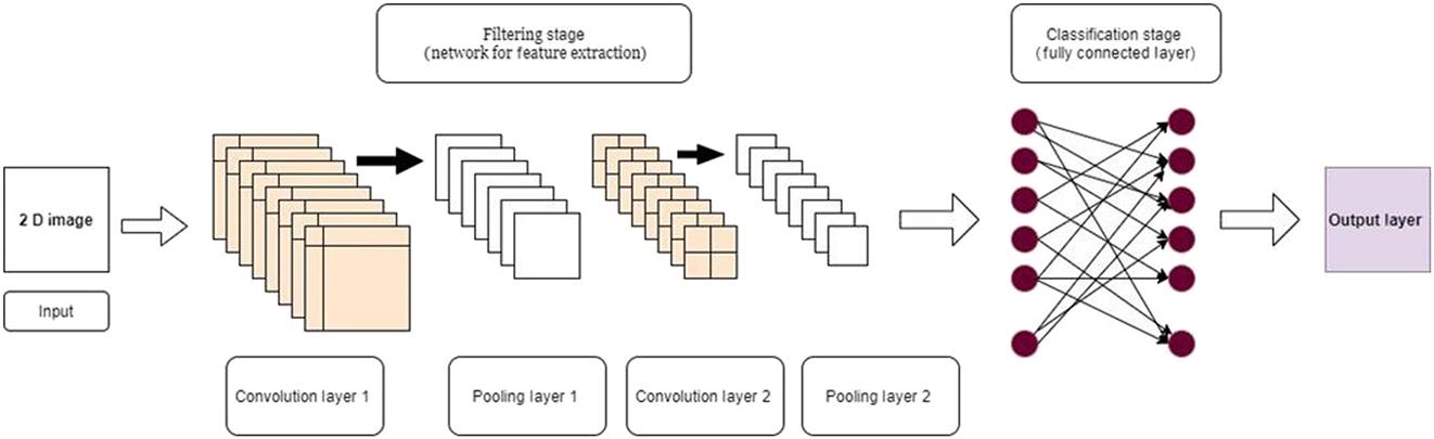
There are three main stages in the convolution operation, two stages of which are for filtering and the third stage is for classification. The architecture or the structure of 2D CNN, as shown in Fig. 3.1, consists one layer of convolutional and the other layer of pooling. To get deep in the network this combination of both layers is repeated in the model. The convolutional and pooling layer is the filter stage of the model. The input in the process is a 2D image of a ball bearing with the fault of any type. The convolutional layer generates a new feature map image from the raw input image. The feature map image includes unique features of the input image by processing the 2D data. This layer contains filters which are called convolution filters. The other filtering stage is a pooling layer which decreases the output image size of convolution filters. Then the output of these two filtering stages (hidden layers) is transferred to the third stage of one or some fully connected layers; the next output from these layers is forwarded to the best classifier to get the detail if the fault is present in the ball bearing. These classifiers are based on SoftMax or Sigmoid functions.

In the literature there are extensive uses of profound learning approaches for fault finding [2,8]. Be that as it may, an enormous named dataset is needed to work with these methodologies. Testing and training of the algorithm are done using the dataset. The computational multifaceted nature is likewise high for these methodologies. To conquer the disadvantages of the high-level methodology of CNN, one-dimensional (1D) CNN is proposed with the upside of less multifaceted nature in calculation as 1D information is prepared in CNN layers.

3.3 1D convolutional neural network

1D CNN is the advanced methodology of conventional CNN. 1D CNN works on 1D vibration signals. Similar to the conventional 2D CNN architecture, this proposed method also consists of two layers. The principal layer is known as the convolutional layer. Both the process of 1D convolution and subsampling happens in first layer. The subsequent layer is the Multi-Layer Perceptron (MLP) layer, which is indistinguishable from the completely associated layer in the regular CNN strategy. Fig. 3.2 shows the architecture or structure of 1D CNN.

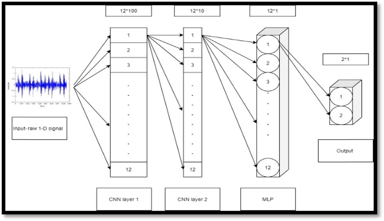
1D CNN is successful for both extraction of features or highlights and the classification of defects or fault embedded in the bearing. Because of this versatile and adaptable design, quite a few layers can be taken practically for hidden layers, and then the subsampling variable or factor of the yield or output CNN layer adaptively selects the number of MLP layers and automatically decides the feature map dimension. As mentioned in Ref. [9], the process of feature extraction and classification of fault of rolling element bearings are integrated into a single 1D CNN. During the period of training of the CNN model, to minimize the error and to maximize the performance of the classification layer, the backpropagation (BP) algorithm is optimized using a gradient descent optimization approach. In the input layer of 1D CNN, there is no necessity for the manual treatment of features or information. 1D CNN layers adjust the information and the feature extraction and subinspecting or subsampling by kernel size, and the feature map is performed by shrouded neurons of the convolution layer. The MLP layer is utilized for classification of the bearing fault. The output from the CNN layer is moved to the MLP layer where the 1D convolution of the 1D signal, along with kernel filter, is executed. Further subtleties including the detailing of the classifier of 1D CNN depending on the BP calculation can be found in Ref. [9].

In 1D CNN [10], as shown in Fig. 3.3, first, the weights are assigned to the neurons, and bias is defined for the CNN layers; afterward, forward propagation is utilized as the yield from the CNN layer, where (l–1) is the contribution to the subsequent shrouded CNN layer l.

$x_k^l=b_k^l+\sum _{i=1}^{N_{l-1}}\mathrm{conv}1\mathrm{D}(w_{ik}^{l-1},S_i^{l-1})$

where $x_k^l$ is input or contribution for layer l from the l–1 layer; $b_k^l$ is bias of $k\mathrm{th}$ neuron of l–1 layer; $w_{ik}^{l-1}$ is kernel from $i\mathrm{th}$ neuron of l–1 layer to the kth neuron at l layer; and $S_i^{l-1}$ is yield of $i\mathrm{th}$ neuron at l–1 layer.

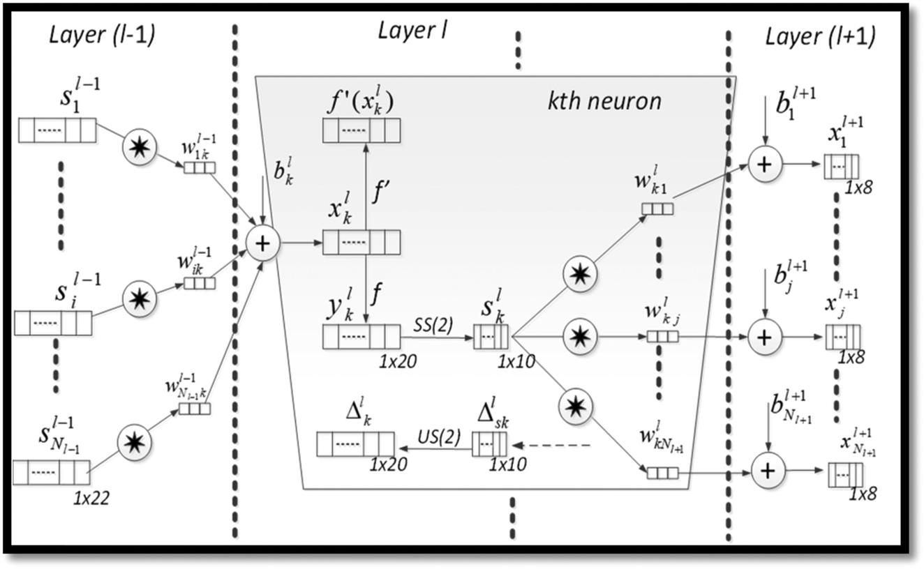
As shown in Fig. 3.2, the yield or output $y_k^l$ is obtained from the input $x_k^l$ of layer l,

$y_k^l=f(x_k^l)\mathrm{and}{s}_k^l=y_k^l\downarrow \mathrm{ss}$

where $s_k^l$ is the after effect of the neuron and is afterward tested with ↓ss activity with the ss factor.

For an error or mistake, BP starts from the yield of the MLP layer. Let l=1 show the input or info layer and l=L is the yield or output layer. Presently, in the information base, the quantity of classes can be considered as $N_n$.

The info vector is p, the objective vector of the input is $t_i^p$, and yield vectors are $[y_1^L,\dots \dots ,y_{N_L}^L]$. The mean-squared error (MSE) in the layer of yield, $E_p$ for input p is characterized as:

$E_p=\text{MSE}\left(t_i^p,\left[y_1^L,\dots \mathrm{.}.,y_{N_l}^L\right]\right)\sum _{i=1}^{N_L}{(y_i^L-t_i^p)}^2$

There are a few errors or mistakes in the model because of organization boundaries. The fundamental focal point of BP is to limit the commitment of boundaries of the organization in mistakes. For the minimization of mistakes, the subsidiary of MSE is figured concerning the individual relegated weight, which is associated with that specific neuron, k. The gradient descent method is applied to limit this commitment of organization boundaries in mistakes. By utilizing the chain rule of subordinate, the bias and weight of the neurons can be refreshed as shown:

$\frac{\partial E}{\partial w_{ik}^{l-1}}={\mathrm{\Delta }}_k^l{y}_i^{l-1}\mathrm{and}\frac{\partial E}{\partial b_k^l}={\mathrm{\Delta }}_k^l$

Further mathematical modeling and the BP algorithm are given in the literature [9–11].

3.4 Statistical parameters for feature extraction

In earlier work, these different features were extracted manually or by any other method in which high expertise was required, and then a different method was used for the classification of the fault in a ball bearing. But nowadays, with this advanced approach of CNN based on deep learning, features are extracted automatically, and then the required feature for further analysis is adaptively selected by the model itself based on the effectiveness and importance of the feature. In Table 3.1, we have presented different features extracted in the literature.

Table 3.1

Statistical parameters for feature extraction [12].

• Feature	• Definition
Mean value	$\overline{x}=\frac{1}{n}\sum _{i=1}^n{x}_i$
Root mean square (RMS)	$\mathrm{RMS}={\left[\frac{1}{n}\left(\sum _{i=1}^n{x}_i\right)\right]}^{1/2}$
Standard deviation	${\sigma }^2=\frac{1}{n-1}\sum _{i=1}^n{(x_i-\overline{x})}^2$
Kurtosis value (KV)	$\mathrm{KV}=\frac{1}{n}\sum _{i=1}^n{\left(\frac{x_i-\overline{x}}{\sigma }\right)}^4$
Crest factor (CF)	$\mathrm{CF}=\frac{\max \left(\left|x_i\right|\right)}{{\left[\frac{1}{n}\left({\sum }_{i=1}^n{x}_i\right)\right]}^{1/2}}$
Inner race ball pass frequency (BPFI)	$\mathrm{BPFI}=f_s\frac{N}{2}\left(1+\frac{D_B}{D_P}\cos \alpha \right)$
Outer race ball pass frequency (BPFO)	$\mathrm{BPFO}=f_s\frac{N}{2}\left(1-\frac{D_B}{D_P}\cos \alpha \right)$
Ball spin frequency (BSF)	$\mathrm{BSF}=f_s\frac{N}{2D_B}\left(1-\frac{D_B^2}{D_P^2}\cos \alpha \right)$
Cage frequency or fundamental train frequency (FTF)	$\mathrm{FTF}=\frac{N}{2}\left(1-\frac{D_B}{D_P}\cos \alpha \right)$

where x is vibration signal; n is number of sampling points; f_s is shaft speed; N is number of balls; D_B is ball diameter; D_P is pitch diameter; and α is contact angle between the inner race and outer race.

3.5 Dataset used

The Machinery Failure Prevention Technology (MFPT) dataset [13] is the openly accessible information for ball bearing flaw finding that is used in this work. For the MFPT dataset, a sort of NICE bearing is utilized in the test rig.

Parameters of ball bearing:

Diameter of ball: 0.23

Pitch diameter: 1.24

Number of balls: 8

Contact angle: 0

The dataset of MFPT is arranged into three segments of bearing vibration data: baseline condition, inner raceway flaw condition, and outer raceway fault conditions. For the pattern set of information, three records are tested for the sample rate of 97,656 Hz for 6 seconds for every document. For the external race flaw condition dataset, seven documents are tested for the sample rate of 48,828 Hz for 6 seconds for each record. Furthermore, for the inward race deficiency condition dataset, seven documents are examined with the sample rate of 48,828 Hz for 3 seconds for every record. All the data in the data were obtained at different load conditions.

3.6 Results

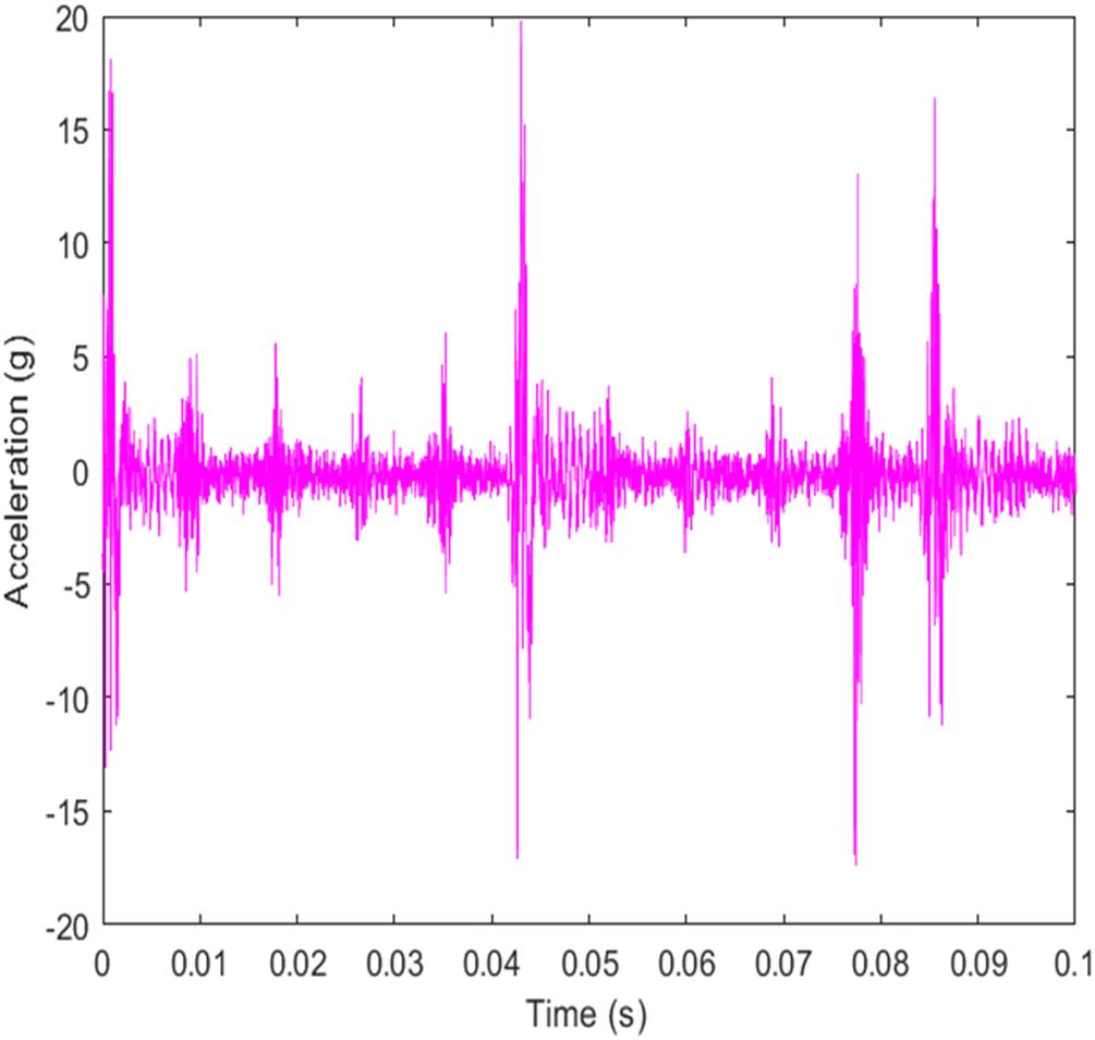
When the ball element of the bearing makes any contact with the fault or defect or flaw at any raceway of the bearing, the implication of hitting the fault will change the corresponding frequency, that is, inner race ball pass frequency (BPFI), outer race ball pass frequency (BPFO), ball spin frequency (BSF), fundamental train frequency (FTF). The raw 1D vibration signal is obtained by an accelerometer in the test rig, and is further analyzed in the 1D CNN layer. Seventy percent of the dataset is utilized for preparing the algorithm and the remaining 30% information of the dataset is utilized for testing the algorithm. Fig. 3.4 shows the crude vibration signal of the condition when the fault is embedded at the inner race of the ball bearing.

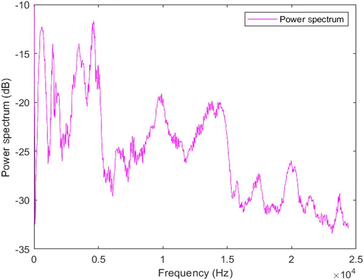
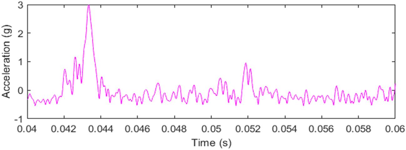
This crude information of the vibration is changed over in the frequency domain or recurrence area, which is anything but difficult to measure in the CNN layer for highlight or feature extraction. In this work, we have mainly focused on performing our analysis for a fault embedded at the bearing inner race. To get a clear visualization of raw data, the vibration information is changed over into the recurrence area or frequency domain, as shown in Fig. 3.5. The sign is then wrapped, as in Fig. 3.6, which depicts the pinnacle modification, through eliminating the noise using the sign. The CNN layer separates the component by convolution, followed by subexamining. What’s more, it adaptively chooses the element as per which class will be chosen. The envelope range of a typical bearing is given to determine the distinction in signs of vibration.

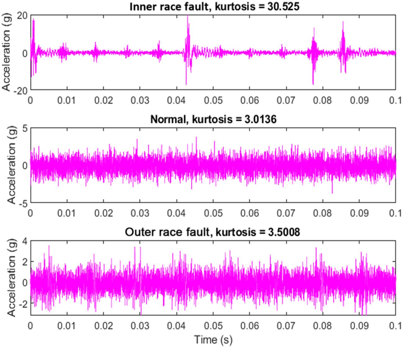
With the help of signals in the time domain, kurtosis is calculated for bearing vibration data. For a random variable, its fourth standardized moment is termed as kurtosis. With the assistance of kurtosis, the impulsiveness or rashness of the sign can be estimated or the substantialness of the tail of the arbitrary variable can likewise be classified. As can be seen in Fig. 3.7, the inner raceway kurtosis is not the same as the ordinary or healthy bearing. Fig. 3.7 arranges the sign picture of kurtosis for the external raceway issue of the bearing, the solid or ordinary bearing, and the inward raceway issue bearing.

To validate the classifier, the testing is done with 30% labeled data of the dataset and the log ratios of the amplitude of BPFI and BPFO correctly describes the accuracy of the system. The effect of the arrangement frameworks is discovered by utilizing evaluation matrices. The outcome from the information can be introduced with regard to evaluation matrices. By and large, flawlessness and precision can be characterized in two classes, one is healthy and the other class is faulty. For any machine component with explicit matrices, classes can be referenced as true positive [TP], true negative [TN], false positive [FP], and false negative [FN]. These networks’ results straightforwardly mirror the effect on state or condition.

The evaluation matrices can be processed as:

		Result
Accuracy	$\mathrm{Acc}=\frac{\left[\mathrm{TP}\right]+\left[\mathrm{TN}\right]}{\left[\mathrm{TP}\right]+\left[\mathrm{TN}\right]+\left[\mathrm{FP}\right]+\left[\mathrm{FN}\right]}$	99%
Sensitivity	$\mathrm{Sen}=\frac{\left[\mathrm{TP}\right]}{\left[\mathrm{TP}\right]+\left[\mathrm{FN}\right]}$	96.1%
Specificity	$\mathrm{Spe}=\frac{\left[\mathrm{TN}\right]}{\left[\mathrm{TN}\right]+\left[\mathrm{FP}\right]}$	98.5%
Positive predictivity	$\mathrm{Ppr}=\frac{\left[\mathrm{TP}\right]}{\left[\mathrm{TP}\right]+\left[\mathrm{FP}\right]}$	97.5%

This methodology of 1D CNN achieved the targets, as the methodology provides results with a high degree of precision when contrasted with the customary strategies. The computational intricate nature of 1D CNN is less for condition monitoring for real-time systems. The purpose behind low computational intricacy is to utilize the 1D arrays, rather than 2D arrays, for the recognition of defects or flaws or faults. There is additionally a low time delay in fault or flaw distinguishing.

3.7 Conclusion

In this work, we have begun with crude vibration signal information collected from an openly accessible MFPT dataset. A deep learning technique-based engineering was planned utilizing convolutional layers, subsampling layers, and MLP layers. The neural network was prepared utilizing 70% of a named dataset and the remaining 30% of the dataset was utilized for testing of the model. Finally, test sets were simulated by using this proposed 1D CNN model. After testing, these results were analyzed and compared with the results from the literature. We further suggest that this strategy can be applied to analyze the fault in ball bearings with high precision and it can be implemented for the constant condition monitoring of bearings.