
Data heterogeneity mitigation in healthcare robotic systems leveraging the Nelder–Mead method
Pritam Khan, Priyesh Ranjan and Sudhir Kumar, Department of Electrical Engineering, Indian Institute of Technology Patna, India
Abstract
Heterogeneity in healthcare data is a cause of concern for the medical professionals. With the increased application of robots in the medical field, data heterogeneity requires to be ad- dressed for improved classification accuracy. In this work, we leverage the Nelder–Mead (NM) optimization method for mitigating data heterogeneity. The NM method is applied on the raw healthcare data to acquire the heterogeneity mitigated data. We classify the electrocardiogram signals from two heterogeneous datasets as normal and abnormal using LSTM (Long Short Term Memory)-based deep learning technique. On mitigating the heterogeneity, the classification accuracies get improved. Therefore the reliability of the robotic healthcare systems increases.
Keywords
Classification; deep learning; healthcare; heterogeneity; robotics
6.1 Introduction
Robotic systems are gaining importance with the progress in artificial intelligence. The robots are designed to aid mankind with accurate results and enhanced productivity. In the medical domain time-series data and image data are used for research and analysis purposes. However, heterogeneity in data from various devices processing the same physical phenomenon will result in inaccurate analysis. Robots are not humans, but are trained by humans, therefore the implementation of the data heterogeneity mitigation technique in the robotic systems will help in improving the performance. In IoT (Internet of Things) networks, heterogeneity is a challenge and various methods are designed for mitigating the problem. The machine learning algorithms that are used for classification, regression, or clustering purposes, are based on the data that are the input to the model. Therefore the data from different devices can yield different classification accuracies.
6.1.1 Related work
Data heterogeneity and its mitigation have been explored in few works. Jirkovzky et al. [1] discuss the various types of data heterogeneity present in a cyberphysical system. The different categories of data heterogeneity are syntactic heterogeneity, terminological heterogeneity, semantic heterogeneity, and semiotic heterogeneity [1]. In that work, the causes of the heterogeneity are also explored. The device heterogeneity is considered for smart localization using residual neural networks in [2]. However, heterogeneity mitigation in the data used for localization would have generated more consistency in the results. Device heterogeneity is addressed using a localization method and Gaussian mixture model by Pandey et al. [3]. Zero-mean and unity-mean features of Wi-Fi (wireless fidelity) received signal strength used for localization assist to mitigate device heterogeneity in Refs. [4] and [5]. The approach is however not used for data classification or prediction purposes from multiple devices using neural networks. The work presented in Ref. [6] aims at bringing interoperability in one common layer by using semantics to store heterogeneous data streams generated by different cyberphysical systems. A common data model using linked data technologies is used for the purpose. The concept of service oriented architecture is introduced in Ref. [7] for mitigation of data heterogeneity. However, the versatility of the data management system remains unexplored.
In this work, we leverage the Nelder–Mead (NM) method for heterogeneity mitigation in the raw data from multiple sources. Mitigation of data heterogeneity from multiple sources will increase the reliability of robotic systems owing to the consistency in prediction, classification, or clustering results. We classify normal and abnormal electrocardiogram (ECG) signals from two different datasets. Although the ECG signals in the two datasets belong to different persons, for the sake of proving the benefit of heterogeneity mitigation, we classify the normal and abnormal ECG signals using Long Short Term Memory (LSTM) from two different datasets.
6.1.2 Contributions
The major contributions of our work are as follows:
- 1. Data heterogeneity is mitigated, thereby increasing the consistency in performance among various devices processing the same physical phenomenon.
- 2. The NM method is a proven optimization technique which validates our data heterogeneity mitigation process.
- 3. A robotic system classifies the normal and abnormal ECG signals with consistency in classification accuracies after mitigating data heterogeneity.
The rest of the paper is organized as follows. In Section 6.2, we discuss the preprocessing of data from two datasets and mitigate the heterogeneity using the NM method. The classification of the ECG data is discussed in Section 6.3. The results are illustrated in Section 6.4. Finally, Section 6.5 concludes the paper indicating the scope for future work.
6.2 Data heterogeneity mitigation
We leverage the NM method for mitigating the data heterogeneity to help the robotic systems yield consistent results from different data sources. This in turn helps the users to increase the reliability of the modern robotic systems. Prior to mitigation of heterogeneity, we need to preprocess the data which can be from different sources.
6.2.1 Data preprocessing
We consider time-series healthcare data analysis in a robotic system. The raw data from various sources can contain unequal numbers of samples owing to different sampling rates and different devices. Therefore we equalize the number of sample-points for each time-series data from different sources. This can be implemented by using the upsampling or downsampling technique. Upsampling is preferred over downsampling to avoid any information loss. The number of sample points from different devices corresponding to a particular time-series data is upsampled to that of the device generating the maximum number of sample points. Once the data from each device contains an equal number of samples, we apply the NM method of heterogeneity mitigation.
6.2.2 Nelder–Mead method for mitigating data heterogeneity
The NM method used for mitigating the instant based intersample distance is robust to noisy signals [8,9]. Using this technique eliminates the necessity of denoising the signals separately in the processing stage. Additionally, this method does not require the knowledge of gradients. The method can be applied when the functions are not locally smooth. NM method minimizes a function of n variables by comparing the function values at (n + 1) vertices of a general simplex and then replacing the vertex with the highest value by another point [9]. An explanation of the NM method with figures is provided in Ref. [9]. A simplex is a generalized figure which can be a point, a line, a triangle, a tetrahedron or any higher dimensional convex hull. If we have initial points xk, 1, xk, 2,…, xk, n from n devices initially, then after NM minimization we have transformed points x′k, 1, x′k, 2,…, x′k, n respectively.
Let us illustrate the NM method used with an example of three sample data points xk, 1, xk, 2, and xk, 3 obtained from three devices. Let the corresponding functions at the three vertices be f (xk, 1), f (xk, 2), and f (xk, 3). In the first iteration, one is assigned to be the worst vertex (say, xk, 1), another to be second worst (say, xk, 2), while the other is the best (say, xk, 3). We can write this as: f (xk, 1)=max if (xk, i), f (xk, 2)=maxi≠1f (xk, i), and f (xk, 3)=mini≠1f (xk, i). Then we calculate the centroid xc for the best side which is opposite to the worst vertex xk, 1.
Now we find the modified simplex from the existing one. As this is a 3-simplex, we have a convex hull of four vertices, that is, a tetrahedron. We replace the worst vertex xk, 1 by a better point obtained with respect to the best side. Reflection, expansion, or contraction of the worst vertex yields the new better point xk, 1. The test-points are selected on the line connecting the worst point xk, 1 and the centroid xc. If the method achieves a better point with a test-point then the simplex is reconstructed with the accepted test-point. However, if the method fails then the simplex is shrunk toward the best vertex xk, 3. Fig. 6.1A describes the reflection technique. The reflection point xk, r is calculated as:
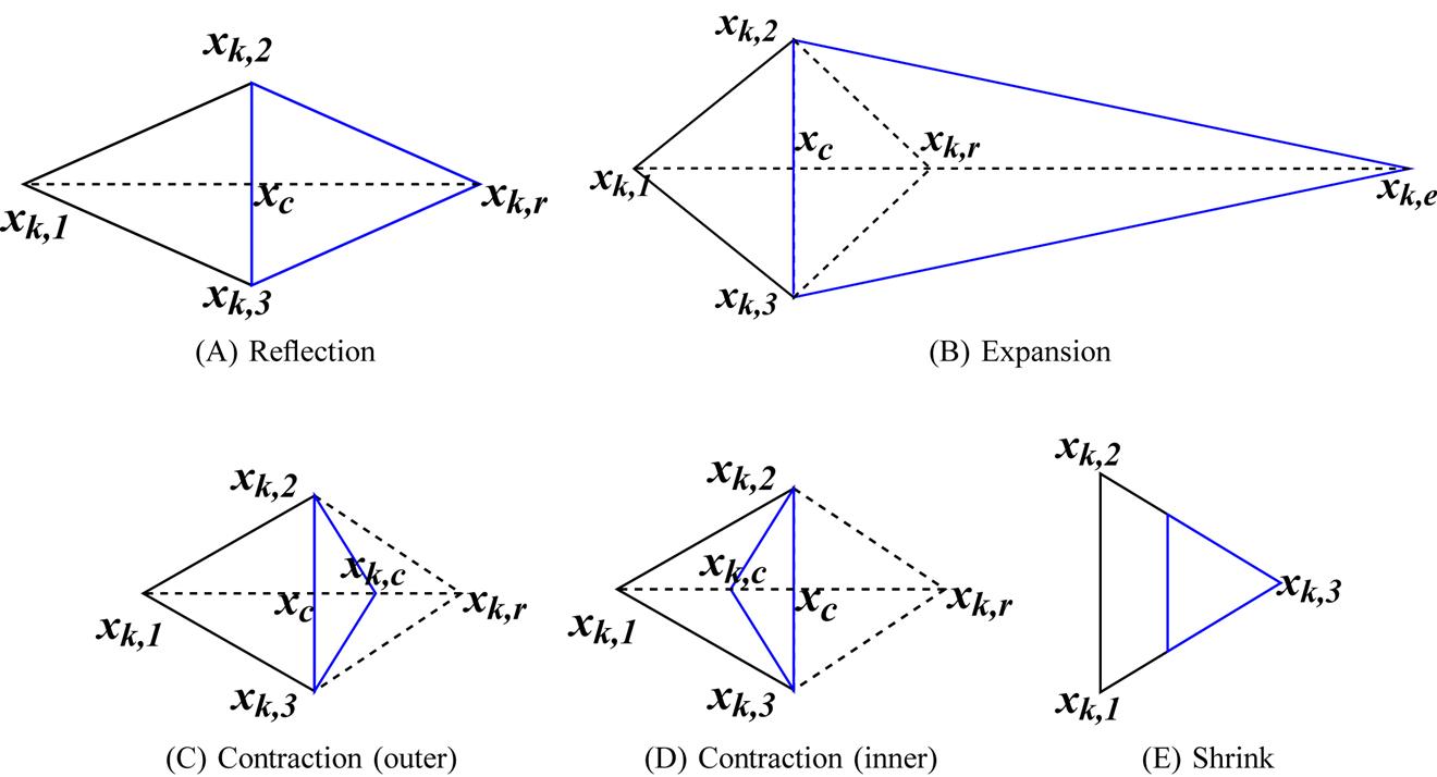
The function corresponding to vertex xk, r is f (xk, r). If f (xk, 3) ≤ f (xk, r) < f (xk, 2), then xk, r is accepted and the iteration is terminated. If f (xk, r) < f (xk, 3), we go for expansion as shown in Fig. 6.1B. The expansion point is computed as:
Now if f (xk, e) < f (xk, r), then xk, e is selected else xk, r is accepted and then iteration is terminated. Hence, a greedy minimization technique is followed. If f (xk, r) ≥ f (xk, 2), then the contraction point xk, c is found using the better point out of xk, 1 and xk, r. If f (xk, 2) ≤ f (xk, r) < f (xk, 1), then contraction is outside the initially considered 3-simplex, as shown in Fig. 6.1C. The contracted point xk, c is given by:
If f (xk, c) ≤ f (xk, r), then xk, c is accepted and iteration is terminated, else we go for the shrink method. However, if f (xk, r) ≥ f (xk, 1), then contraction is considered inside the initially considered 3-simplex as shown in Fig. 6.1D. In this case we get the contracted point xk, c as:
If f (xk, c) < f (xk, 1), then xk, c is accepted and iteration is terminated, else we perform the shrink operation as shown in Fig. 6.1E. In the shrink method, we obtain all the new vertices as:
Shrinking transformation is used when contraction fails due to the occurrence of a curved valley causing some point of the simplex to be much further away from the valley bottom than the other points. This transformation finally brings all the points into the valley. Based on the values of sample points xk, 1, xk, 2, and xk, 3 from three different devices, the NM method uses expansion, contraction, or shrinking to obtain a new set of transformed points x′k, 1, x′k, 2, and x′k, 3, respectively.
Here we illustrate the NM minimization using a 3-simplex, that is, data from three different devices. However, this can be generalized for any higher or lower order simplex. For example, if we consider two devices, then we have 2-simplex, that is, a triangle, and if we consider four devices, then we have a pentagon for evaluation.
The NM method must terminate after a certain period of time. Three tests are conducted to terminate the NM method [8,9]. If any of them is true then the NM method stops operating. The domain convergence test yields positive results if all or some vertices of the present simplex are very near to each other. The function-value convergence test is true if the functions at different vertices are very close to each other. Finally, the no-convergence test becomes positive if the number of iterations exceeds a certain maximum value.
6.3 LSTM-based classification of data
LSTM is a special category of recurrent neural network aimed at handling time-series data. We classify the ECG signals into normal and abnormal in this work using LSTM. Our objective is to show that there is consistency in classification accuracy for heterogeneity mitigated data over heterogeneous data in robotic systems. The computational complexity of LSTM is of the order of O(1) per time step and weight. LSTM has a recurrently self-connected linear unit called “constant error carousel” (CEC). The recurrency of activation and error signals helps CEC provide short-term memory storage for the long term [10,11]. In an LSTM unit, the memory part comprises a cell and there are three “regulators” called gates, controlling the passage of information inside the LSTM unit: an input gate, an output gate and a forget gate [12]. LSTM works in four steps:
- 1. Information to be forgotten is identified from previous time step using forget gate.
- 2. New information is sought for updating cell state using input gate and tanh.
- 3. Cell state is updated using the above two gates information.
- 4. Relevant information is yielded using output gate and the squashing function.
In Fig. 6.2, LSTM-dense layer-softmax activation architecture is illustrated.
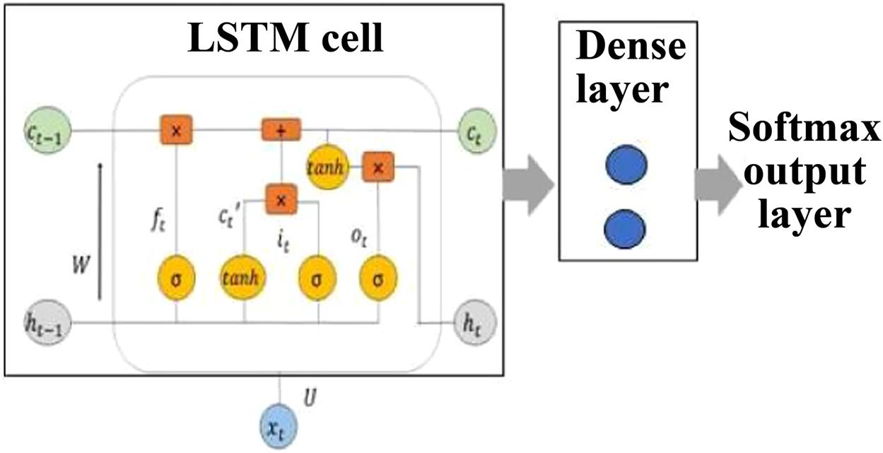
Let xt be the input received by the LSTM cell in Fig. 6.2. it, ot, and ct represent input gate, output gate, and long-term memory of current time-step t, respectively. W and U are weight vectors for f, c, i, and o. The hidden unit (ht) at each time-step learns which data to keep and which to discard. Accordingly, the forget gate (ft) keeps a 0 (to forget entirely) or a 1 (to remember). Hence, the activation function in the forget gate is always a sigmoid function (σ).
Further, we require to evaluate the information learnt from xt where the activation function is generally tanh.
Now prior to addition of the information to memory, it is necessary to learn which parts of the information are not redundant and are required to be saved through the input gate it. Here also the activation function is σ.
Thus the working memory is updated and the output gate vector is learnt.
The present cell state is obtained as
And the present hidden unit as
In Fig. 6.2, LSTM cell output is given to a dense layer. The softmax activation function is given to the output stage after the dense layer. Softmax activation function for any input vector y comprising n elements is given by: ![]() where
where ![]() .
.
In ECG data classification, information about the previous state is required in the present state for accurate classification of activities.
6.4 Experiments and results
We use the data from the Massachusetts Institute of Technology-Beth Israel Hospital (MIT-BIH) arrhythmia database and Physikalisch-Technische Bundesanstalt (PTB) Diagnostic ECG database to mitigate heterogeneity and further classify them into normal and abnormal categories [13–15]. An amalgamation of both the databases is carried out as it contributes to heterogeneity. We select those ECG waveforms from both the datasets with the R peaks at approximately the same positions by mapping. Finally, we train and test the LSTM with the selected parts of the MIT-BIH dataset and the PTB database. Next we mitigate the heterogeneity between MIT-BIH and PTBDB data using NM method as observed from Table 6.1. Heterogeneity mitigation leads to increase in accuracy during classification.
Table 6.1
MIT-BIH, Massachusetts Institute of Technology-Beth Israel Hospital; NA, Not applicable.
6.4.1 Data heterogeneity mitigation using Nelder–Mead method
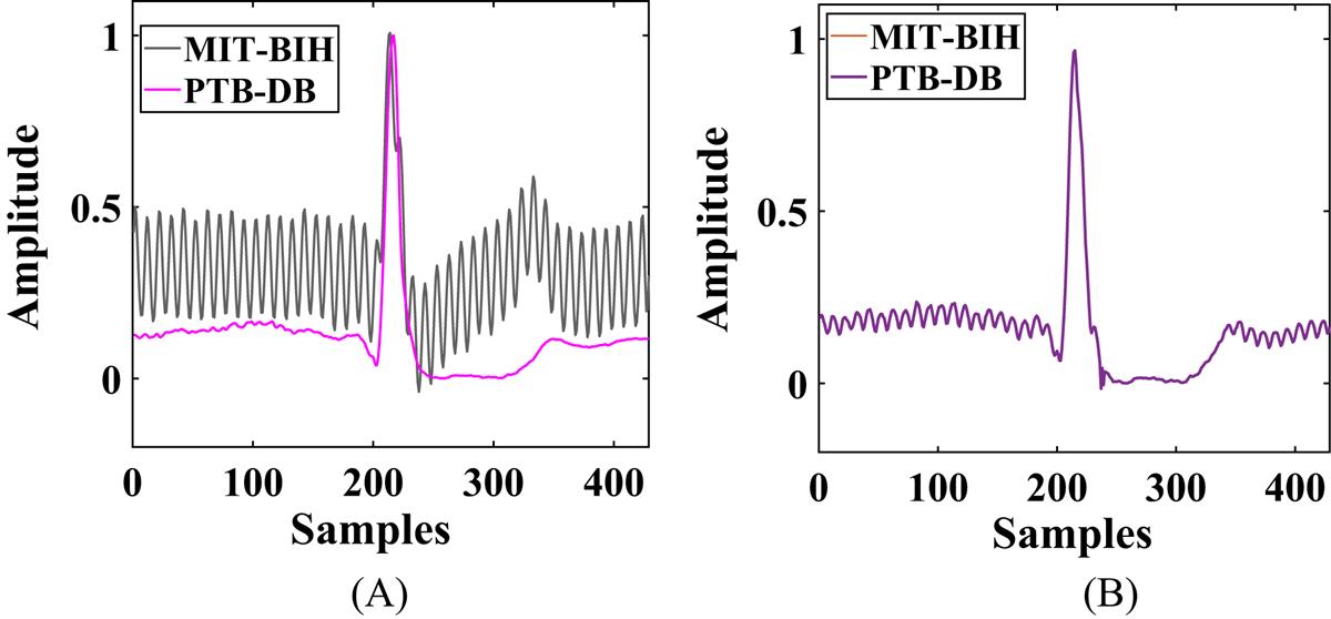
One beat of an ECG waveform is chosen from both the datasets as shown in Fig. 6.3A, whose heterogeneity when removed gives the waveforms as shown in Fig. 6.3B corresponding to the NM method. We calculate the RMSE (root mean squared error) between the two ECG waveforms, as shown in Fig. 6.3A and B. Fig. 6.3B represents the RMSE for the same beat of ECG from two devices after heterogeneity mitigation using the NM method [8,9]. For Fig. 6.3A we have RMSE=2.390×10⁻¹. Using the NM method, we can reduce the RMSE to 1.008 × 10⁻⁵. The RMSE is calculated for 8000 iterations and the time taken by the NM method for the same is 1.436 seconds. Notably, RMSE is very small since the signals are normalized between 0 and 1.
6.4.2 LSTM-based classification of data
Leveraging data from different sources lead to data heterogeneity. In this work, we use two different ECG datasets for classification where each dataset comprises data from different persons acquired using different devices of different specifications. We classify the ECG data from the two datasets namely MIT-BIH and PTB-DB separately as well as in combined states. We create a fusion of the normal classes from the two databases and similarly of the abnormal classes also, thereby creating a heterogeneous platform of data. The LSTM-softmax deep learning model is used for classification purpose. In order to achieve the best performance using the LSTM model, we tune the hyperparameters like number of LSTM hidden units and batch size, and regularize the model using the ![]() 2 norm of regularization. Both the number of hidden units and batch size are tuned to 64 for the LSTM model. The learning rate is selected as 0.01 for maximizing the accuracy of our model. Also, we select the rate for
2 norm of regularization. Both the number of hidden units and batch size are tuned to 64 for the LSTM model. The learning rate is selected as 0.01 for maximizing the accuracy of our model. Also, we select the rate for ![]() 2 norm of regularization as λ=0.001.
2 norm of regularization as λ=0.001.
The performance evaluation of the classification model based on test data is carried out using a confusion matrix [16]. We obtain the following performance metrics from the confusion matrix.

where TP, TN, FP, and FN represent True Positive, True Negative, False Positive, and False Negative, respectively. Another performance metric called F1 score is calculated from precision and recall values. F1 score is the weighted average of accuracy and recall and it varies from 0 to 1. It is defined as follows:
All the evaluation parameters, namely, precision, recall, and F1 score, are tabulated in Table 6.1 in addition to training and testing accuracies. From Table 6.1, it is observed that the NM method-based heterogeneity mitigated data yields a training accuracy of 91.84% and a test accuracy of 91.67%, which are higher than that for heterogeneous data (MIT-BIH and PTB-DB combined). The heterogeneous data has a maximum training accuracy of 90.31% and a test accuracy of 86.18%. We also evaluate our model in terms of other performance metrics like precision, recall, and F1-score.
However, when we consider each dataset separately for classification of ECG signals into normal and abnormal separately, we get higher accuracy, as observed from Table 6.1.
Therefore when we implement the heterogeneity mitigation method, we trade-off accuracy to some extent at the expense of increasing reliability on the robotic system. A robotic system yielding the results as shown in Fig. 6.3B is more reliable and consistent compared to that in Fig. 6.3A.
6.5 Conclusion and future work
In this work, we mitigate the heterogeneity in the data that is analyzed by a robotic system. Mitigation of data heterogeneity is carried out using the NM optimization technique. It is observed from the results that the RMSE reduces by a large extent among the heterogeneity mitigated data as compared to heterogeneous data. Additionally, we classify the healthcare ECG data from two datasets, namely MIT-BIH and PTB-DB, into normal and abnormal categories. We use the LSTM-softmax deep learning model for classification purposes. The NM method-based heterogeneity mitigated data yield higher classification accuracies in comparison to the heterogeneous data.
We are carrying out further research to mitigate the heterogeneity for multivariate healthcare data in robotic systems. Most of the healthcare conditions require multiparameter monitoring. Therefore the robots need to be trained with algorithms capable of handling multivariate analysis with the data heterogeneity mitigated.
Acknowledgment
This work acknowledges the support rendered by the Early Career Research (ECR) award scheme project “Cyber-Physical Systems for M-Health” (ECR/2016/001532) (duration 2017–20), under Science and Engineering Research Board, Government of India.