Keywords

Inverse kinematics; DOF (degree of freedom); transformation; DH convention; robotic arm; PSO; firefly

2.1 Introduction

Industrial robots are playing a vital role in the manufacturing industry. They are generally used as payloader, welding, painting, assembly, packaging, and other important applications. These types of robots are automated, programmable as well as can move in all three dimensional axes. The end effector of an industrial robot is one of the vital parts of the robot which is used by the robot to communicate with the environment. Therefore to place the end effector in the right position at the right time is the most challenging job for an industrial robot. The classical method to find the position of an end effector is by solving the inverse kinematics. Generally, massive numerical calculations need to be solved to get the answer for the position of the end effector. However, with the evolution of computing, solving the calculations has become easier as well as quicker. But, for an automated industrial robot, speed is a significant parameter of operation. Researchers are trying to develop faster robots to manufacture more commodities in shorter time periods. Recent developments in the field of Artificial Intelligence and machine learning allow deriving faster calculation and consequently developing faster robots. Therefore this opens a new era in robotics with the applications of Artificial Intelligence and machine learning.

In this chapter, we have analyzed a 7-degree of freedom (DOF) robotic manipulator with the help of D-H convention by establishing different parameters of robotic manipulators. Further, we have used Catia V5 Pro software for modeling and positioning different end-effector and manipulator positions. We have taken a number of end effectors positions (target) to calculate the joint angles. We have employed two swarm optimization: Particle Swarm Optimization (PSO) and Firefly Algorithm (FA) to find the joint angels for a given target. With the selection of random points in the workspace we have run the simulation to achieve the predetermined accuracy.

2.2 Literature review

Finding the location of the joints for the given end effector position, that is, inverse kinematics problems is a classical problem in the robotics [1,2]. As the end effector position can be written as a function of the location of the joint position, finding the inverse solution involves trigonometrical and nonlinear function, and getting the solution for a multiple DOF system becomes increasingly difficult. This problem can be solved with the help of numerical or computational methods. Classical optimization techniques were being used for solving such problems but they don’t lead to the desired accuracy.

In the last 20 years many metaheuristics methods including the Cuckoo search method [3] have evolved and are being implemented for solving industrial problems. The Cuckoo search method is based on the assumption that each cuckoo will lay an egg in one nest and the best egg will be used as the new solution and rest will be discarded. This method is very helpful for providing the best solution.

In the literature [4–6] we find neural network, bee algorithm, and genetic algorithm being used to solve inverse kinematics problems. Similarly, PSO [7] and FA [8] were used to get the joint parameters for the given end effector positions.

Apart from inverse kinematics problems there are numerous other applications of robotics, such as navigation and control [9], energy minimization [10] during movement, and trajectory planning [11], where metaheuristic optimizations are being implemented to solve the problems. Recently, artificial intelligence-based optimization has also been used [12–15].

2.3 Modeling and design

For the analysis of a robot, first the workspace, link length, joint angle, etc. are to be defined. Using forward kinematics with the use of mathematical equations the end effector position is determined. As we increase the number of DOFs the mathematical complexity increases and solving inverse kinematics becomes challenging. Many algorithms are being used to solve such problems but still for higher DOF problem inverse kinematics is not a done deal.

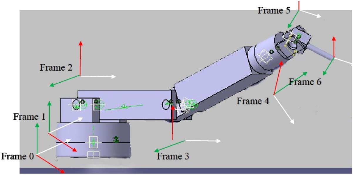
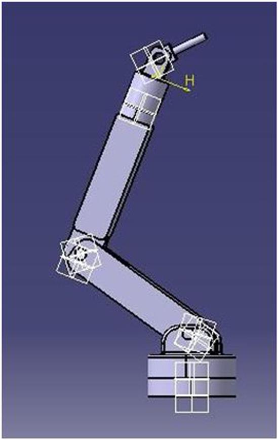
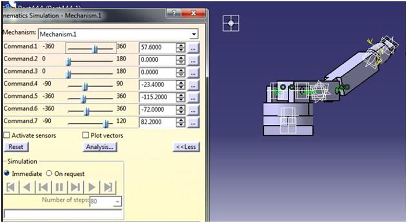
We have started with the assigning of D-H parameters for the model. For modeling the 7-DOF robot we have employed CATIA modeling software, and using different features we have accurately shown the link and end effector position, as depicted in Figs. 2.1–2.3.

2.3.1 Fitness function

The aim of this work is to reach the desired position of the end effector from the initial input. We reduced the problem to an optimization problem with given fitness function. Essentially our approach here is to formulate the problem as an optimization problem with the target of minimizing the fitness function. We set the target to minimize the error iteratively.

$F=\sqrt{{(X_{\mathrm{T}}-X)}^2+{(Y_{\mathrm{T}}-Y)}^2+{(Z_{\mathrm{T}}-Z)}^2}$

In the above expression F is chosen to be fitness function; X_T is the target position of the end effector in the x direction; Y_T is the target position of the end effector in the y direction; and Z_T is the target position of the end effector in the z direction. Here we have chosen the fitness function as the Euclidian distance between the target location and the present location of the end effector.

2.3.2 Particle swarm optimization

The PSO method was first proposed in 1995 by Kennedy [16]. The optimization technique is governed by personal best and global best.

In this algorithm first we define swarm size, and then we decide about the search space number of iteration etc. Further we place the position of the particle randomly and define the position too. The fitness function is calculated each time. Then the personal and global best of the fitness function is updated. Then the velocity and position of the particle is determined using the given equation each time. Finally stopping criteria is checked after running each iteration.

The updated position (x_i(t+1)) of the particle is a function of the last position (x_i(t)) of the particle and the velocity at the current location:

$x_i(t+1)=x_i(t)+v_i(t+1)$

And the updated velocity of the particle is given by:

$v_{ij}(t=1)=w{v}_{ij}(t)+c_1{r}_1(p_{\mathrm{best}}-x_{ij}(t))+c_2{r}_2(g_{\mathrm{best}}-x_{ij}(t))$

where r₁ and r₂ are random numbers, and w is inertia weight.

The algorithm can be stated as followed. First, create a collection of the swarm on a random basis. Then evaluate the value of the fitness function for each particle, then iterate and update velocity. Further, update the position. Then, select the best solution (position) by calculating and updating the position and velocity. Finally, check accuracy and stop if the criteria are met.

The fitness function is chosen as the Eulerian square of the difference between the actual angles and calculated angles.

2.3.3 Firefly algorithm

The firefly optimization technique is another algorithm inspired by nature. Yang [3] proposed a method of optimization which mimics the behavior of fireflies. FA is being implemented nowadays to solve some of the most complex problems of mathematics, supply chains, and finance. The method is statistical and uses random variables. Fireflies of a particular type flash lights to attract another butterfly for mating, as potential prey, or other purposes.

The assumption in the fireflies algorithm is as follows: the firefly with lower intensity moves toward the brighter intensity and it decreases with the distance. The calculation of the fitness function is an indicator of the brightness.

The light intensity can be presented as:

$I=I_0{e}^{-\gamma r}$

The measure of attractiveness can be written as:

$\beta ={\beta }_0{e}^{-\gamma r}$

Movement of the firefly can be expressed as:

$x_i=x_i+{\beta }_0{e}^{-\gamma r^2}(x_j-x_i)+\alpha {\epsilon }_i$

where ${\beta }_0$ is the attractiveness when r=0; no of fireflies is 50; light absorption coefficient ($\gamma$) is 0.8; attraction coefficient base value is 0.25; mutation coefficient is 0.2; mutation coefficient damping ratio is 0.997; and uniform mutation range is 0.8.

2.4 Results and discussions

The coding was done for PSO and FA in MATLAB [17]. The initial population for the swarm was taken randomly inside the workspace of the robotic system.

The parameters for the two algorithms were taken as per data provided in the earlier sections. The fitness function has been selected as the Euler’s distance between the target position and the latest position of the end effector.

Our aim here was to minimize the error and converge to an optimal solution for each joint position. The related parameters were updated each time and checked for the convergence.

The accuracy for the simulation was selected as 10⁻⁴.

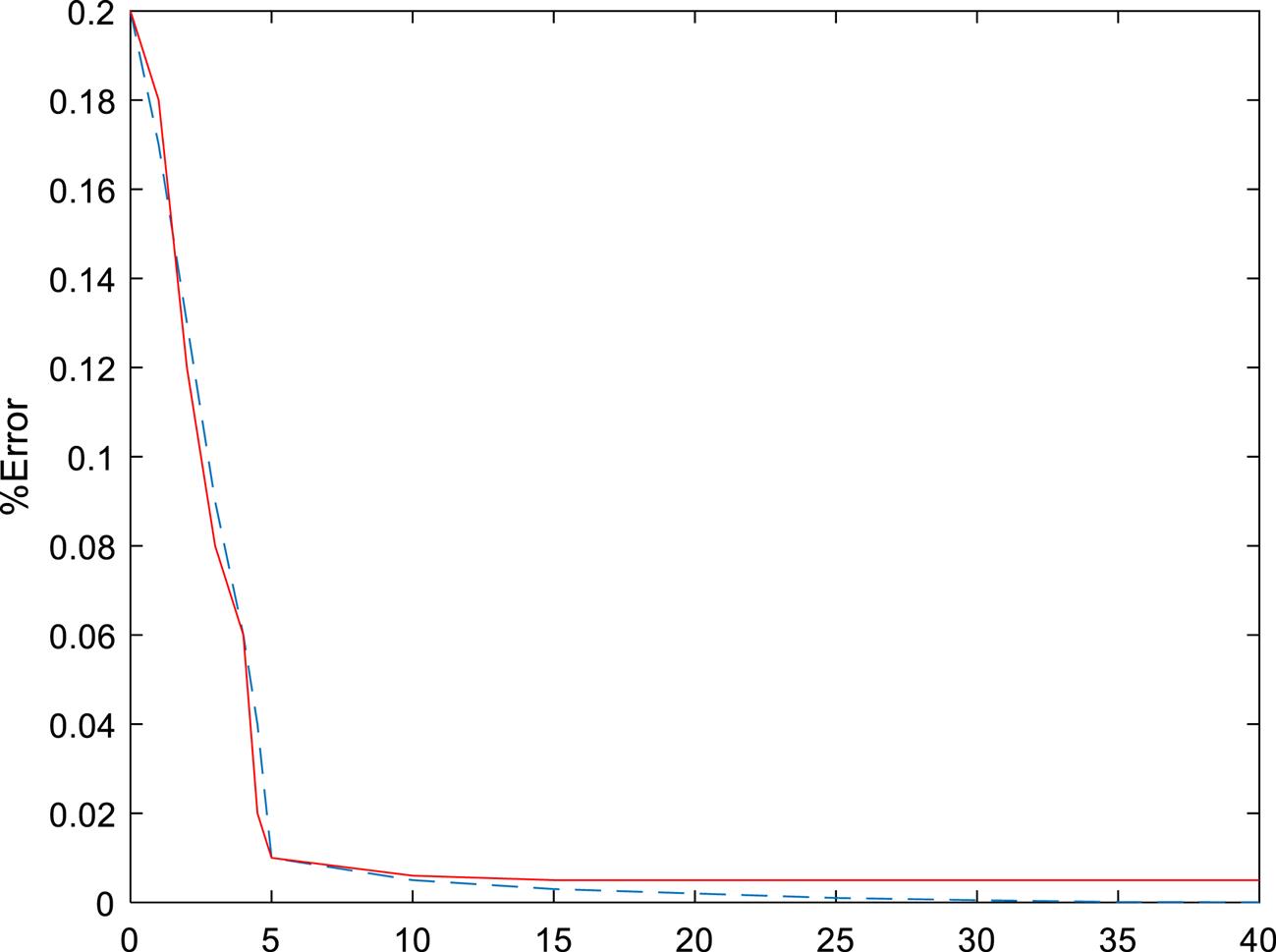
The result is shown in the plot [4] generated through the MATLAB coding. From the plot it can be seen that PSO algorithm gives accuracy of over 10⁻⁸ comparison in just 40 iterations, whereas the FA gives an accuracy of 10⁻⁴ after 110 iterations Fig. 2.4.

2.5 Conclusions and future work

In the present work, we have used optimization techniques to find the joint angles of the robot for a 7-DOF robot for end effector position. We started with randomly selecting 100 points in the robotic workspace and ran the simulation in two different optimization algorithms: PSO and FA. After running the simulations, it was found that PSO outperformed FA as PSO took just 40 iterations to achieve the accuracy of 10⁻⁸ compared to firefly which took 110 iterations to achieve just 10⁻⁴ accuracy.

In future the present work can be extended for even more DOFs and some other newly developed metaheuristic algorithms can be employed to get better solution with even fewer iterations. Some real-time data can help to find the efficacy of the present method. Furthermore, two or more optimization methods can be employed and a hybrid method can be employed to get better accuracy.