
4
Machine Evolution
4.1 Evolutionary Computation
The systems we studied in the last chapter adapt their behaviors so that they conform to a set of training instances. This type of learning mimics some aspects of learning in biological systems. Another way in which biological systems adapt is by evolution: generations of descendants are produced that perform better than do their ancestors. Can we use processes similar to evolution to produce useful programs? In this chapter, I examine a technique that attempts to do just that.
Biological evolution proceeds by the production of descendants changed from their parents and by the selective survival of some of these descendants to produce more descendants. These two aspects, change through reproduction and selective survival, are sufficient to produce generations of individuals that are better and better at doing whatever contributes to their ability to reproduce. The following geometric analogy portrays a simplified version of the process: imagine a mathematical “landscape” of peaks, valleys, and flat terrain populated by a set of individuals located at random places on the landscape. The height of an individual on this landscape is a measure of how well that individual performs its task relative to the performance of the other individuals. Those individuals at low elevations cease to exist, with a probability that increases with decreasing height. Those individuals at high elevations “reproduce” with a probability that increases with increasing height. Reproduction involves the production of new individuals whose location on the landscape is related to, but different from, that of the parent(s). The most interesting and efficacious kind of reproduction involves the production of new individuals jointly by two parents. The location(s) of the offspring on the landscape is a function of the locations of the parents. In some instantiations of the evolutionary process, the location of an offspring is somewhere “between” (in some sense) the locations of the parents.
We can regard this process as one of searching for high peaks in the landscape. Newly generated individuals sample new terrain, and those at the low elevations die off. After a while, some individuals will be located on peaks. The efficiency of the exploration process depends on the way in which an individual differs from its parent and on the nature of the landscape. Offspring might have elevations lower than their parents, but some might occasionally be higher.
Evolutionary search processes have been used in computer science for two major purposes. The most straightforward application is in function optimization. There, we attempt to find the maximum (say) of a function, f(x1, …, xn). The arguments (x1, …, xn) specify the location of individuals, and the value f is the height. John Holland [Holland 1975] proposed a class of genetic algorithms (GAs) for solving problems of this sort. GAs are well described in various textbooks and articles. (See, for example, [Goldberg 1989, Mitchell, M. 1996, Michalewicz 1992].)
The other application is to evolve programs to solve specific problems—for example, programs to control reactive agents. This is the application that concerns us here. Elaborations on GAs called classifier systems [Holland 1986], [Holland 1975, pp. 171ff, 2nd ed.] have been used successfully for this purpose. Another technique, called genetic programming (GP) [Koza 1992, Koza 1994], evolves programs in a somewhat more direct manner than do GAs. In the next section, I will illustrate the GP process with an example.
4.2 Genetic Programming
4.2.1 Program Representation in GP
In GP, we evolve functional programs such as LISP functions. Such programs can be expressed as rooted trees with labeled nodes. Internal nodes are functions, predicates, or actions that take one or more arguments. Leaf nodes are program constants, actions, or functions that take no arguments. I show an example of how a program for computing 3 + (5 × 4)/7 is expressed as a tree in Figure 4.1. In this case, the leaf nodes are the constants 3, 4, 5, and 7, and the internal nodes are the functions +, ×, and /.

Figure 4.1 A Program Expressed as a Tree
Here, I show how GP can be used to evolve a wall-following robot whose task is the same as that considered in Chapter 2. Suppose the world for this robot is the two-dimensional grid world shown in Figure 4.2. We want to evolve a program that takes as inputs the robot’s current sensory data and computes a single action. The robot is controlled by repeated execution of this program, and we want repeated execution to move the robot from an arbitrary initial position to a cell adjacent to the wall and then to follow the wall around forever.

Figure 4.2 A Robot in a Grid World
The primitive functions to be used in the program include four Boolean functions, AND, OR, NOT, and IF; and four actions, north, east, south, and west. The Boolean functions have their usual definitions:
The actions are defined as before:
1. north moves the robot one cell up in the cellular grid
2. east moves the robot one cell to the right
The action functions themselves have effects but no values; the evaluation of any of them terminates the program so that there is no need to pass a value up the tree. All of the action functions have their indicated effects unless the robot attempts to move into the wall; in that case, the action has no effect except to terminate the program. Of course, repeating the execution of a program that terminates with no effect will also have no effect.
We use the same sensory inputs as before. Here, rather than using the s1, …, s8 notation, I use the more mnemonic n, ne, e, se, s, sw, w, and nw. These inputs have value 0 whenever the corresponding cell is free for the robot to occupy; otherwise, they have value 1. Figure 4.2 shows the locations of the cells being sensed relative to the robot.
For GP, we must ensure that all expressions and subexpressions used in a program have values for all possible arguments (unless execution of an expression terminates the program). For example, if we were to use the function Divides(x, y) to denote the value of x divided by y, we will need to give it some value (perhaps 0) when y is 0. In this way, we ensure that any tree constructed so that each function has its proper number of arguments describes an executable program. We will see later why this point is important.
Before proceeding to use GP to evolve a wall-following program, I show an example of a wall-following program in Figure 4.3; I show both the tree representation and the equivalent list-structure representation. Repeated execution of the program will cause the robot to go north to the wall and follow it around in a clockwise direction. This program can be compared with the production system for boundary following developed in Chapter 2.
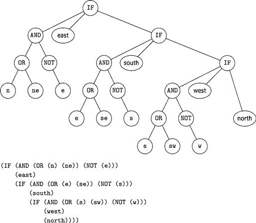
Figure 4.3 A Wall-Following Program
4.2.2 The GP Process
In genetic programming, we start with a population of random programs, using functions, constants, and sensory inputs that we think may be the ones that will be needed by programs if they are to be effective in the domain of interest. These initial programs are said to constitute generation 0. The size of the population of programs in generation 0 is one of the parameters of a GP run. In my illustration of how GP works, we are going to start with 5000 random programs and attempt to evolve a wall-following robot. We produce these initial random programs from the primitive functions AND, OR, NOT, and IF, the actions north, east, south, and west, the sensory functions n, ne, e, se, s, sw, w, nw, and the constants 0 and 1. Programs in each generation are evaluated, and a new generation is produced until a program is produced that performs acceptably well.
A program is evaluated by running it to see how well it does on the task we set for it. In our case, we run a program 60 times and count the number of cells next to the wall that are visited during these 60 steps. (There are 32 cells next to the wall, so a program that never gets to the wall would have a count of 0, and a perfect program would have a count of 32.) Then we do ten of these runs with the robot starting in ten randomly chosen starting positions. The total count of next-to-the-wall cells visited during these ten runs is then taken as the fitness of the program. The highest possible fitness value will be 320—achievable only by a robot that on each of its ten fitness runs visits all of the next-to-the-wall cells within 60 steps.
The (i + l)–th generation is constructed from the i-th one in the following manner:
1. Five hundred programs (10%) from generation i are copied directly into generation i + 1. Individuals are chosen for copying by the following tournament selection process: seven programs are randomly selected (with replacement) from the population of 5000. Then the most fit of these seven programs is chosen. (Tournament selection has been found to be an efficient method for selecting fit individuals. The number 7 and the percentage of programs to be copied are additional parameters of the GP process.)
2. Forty-five hundred new child programs (90%) are put into generation i + 1. Each child program is produced from a mother and a father program by a crossover operation as follows: a mother and a father are each chosen from generation i by tournament selection (as before). Then a randomly chosen subtree from the father replaces a randomly selected subtree from the mother. The result is the child program. (Executability of the child is guaranteed by the requirement that all functions used in the programs be executable for all possible values of their arguments.) I show an illustration of the crossover operation in Figure 4.4. The shaded node in each parent has been selected as a crossover point. The child program may or may not have higher fitness than its parents. The motivation for the possible effectiveness of the crossover operation is that a main program and a subexpression of fit parents are incorporated into their child.

Figure 4.4 Two Parent Programs and Their Child
3. Sometimes a mutation operator is also used in constructing individuals for the next generation. When used, it is used sparingly (perhaps at a 1% rate). The mutation operator selects a single parent from generation i by tournament selection (as before). A randomly chosen subtree is deleted from this parent and replaced by a newly grown random subtree (created in the same manner as individuals are created for generation 0). My illustrative example does not use mutation.
Note that several rather arbitrary parameters must be set in constructing the next generation. These include the number of individuals to be copied, the number to be produced by crossover, the number used in tournament selection, and the mutation percentage. The parameters used here in my illustrative experiment are based on the recommendations of experts in the technique of genetic programming.
4.2.3 Evolving a Wall-Following Robot
Starting with our population of 5000 random programs, and using the techniques just described, we start the GP process for evolving a wall-following robot.1 Many of the random, generation 0 programs do nothing at all: for example, (AND (sw) (ne)) (with fitness = 0) evaluates its first argument, terminates if the result is 0, and otherwise evaluates its second argument and terminates. Some programs move in one direction only regardless of their inputs. For example, when program (OR (e) (west)) evaluates west, it moves west and terminates. That program had a fitness of 5 (some of its random runs happened to traverse cells next to the wall). The 5000 programs in generation 0 can be regarded as an uninformed search of the space of computer programs using ingredients chosen for this particular problem class.
The list-structure form of the most fit program of generation 0 (fitness = 92) and two of its fitness runs are shown in Figure 4.5. As is usual with GP, the program is rather difficult to read and has many redundant operations. (Some of these might be removed by a postprocessing translator.) Starting in any cell, this program moves east until it reaches a cell next to the wall; then it moves north until it can move east again or it moves west and gets trapped in the upper-left cell.
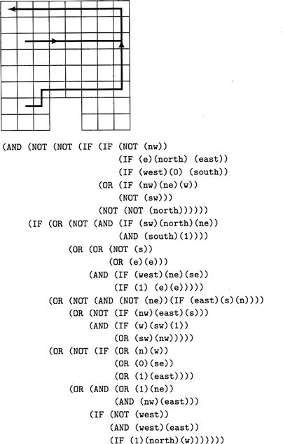
Figure 4.5 The Most Fit Individual in Generation 0
The best program of generation 2 has a fitness of 117. The program and its performance on two typical fitness cases are shown in Figure 4.6. The program is smaller than the best one of generation 0, but it does get stuck in the lower-right corner.

Figure 4.6 The Most Fit Individual in Generation 2
By generation 6, performance has improved to a best fitness of 163. The best program follows the wall perfectly but still gets stuck in the bottom-right corner, as shown in Figure 4.7.
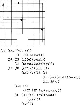
Figure 4.7 The Most Fit Individual in Generation 6
Finally, by generation 10, the process has evolved a program that follows the wall perfectly. This program and two of the paths it takes from different starting positions are shown in Figure 4.8. The program follows the wall around clockwise and moves south to the wall if it doesn’t start next to it.

Figure 4.8 The Most Fit Individual in Generation 10
I show in Figure 4.9 a curve of the fitness of the most fit individual in each generation. Note the progressive (but often small) improvement from generation to generation.
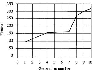
Figure 4.9 Fitness as a Function of Generation Number
4.3 Additional Readings and Discussion
Genetic algorithms and genetic programming have been applied in a variety of settings. GP methods have successfully evolved reactive agents similar to those studied by other AI researchers. These include box pushing, ant trail following, truck trailer backing, and inverted pendulum balancing. These and other demonstrations of the versatility of the technique are described in [Koza 1992]. Added power is gained when the method is extended to allow the evolution of subroutines that can subsequently be used by the coevolving main program just as if they were primitive functions. This feature and its applications are presented in [Koza 1994]. Perhaps the most complex and successful applications of GP are in synthesizing electronic filters, amplifiers, and other circuits [Koza, et al. 1996]. Some preliminary work has also been done on GP methods for evolving programs that create and use memory structures, that search, and that employ recursion [Andre 1995, Teller 1994, Brave 1996].
Genetic programming and genetic algorithms research papers appear in Proceedings of the Conferences on Genetic Programming, the IEEE Transactions on Evolutionary Computation, and the Proceedings of the International Conferences on Genetic Algorithms.
Exercises
4.1 Specify fitness functions for use in evolving agents that
2. Control stop lights on a city main street
4.2 Determine what the words genotype and phenotype mean in (biological) evolutionary theory. How might these words be used to describe GP?
4.3 How might the GP crossover process be changed to allow GP to relax the requirement that the execution of every subtree return a value?
4.4 The crossover operation used in GP selects a random subtree in both parents. Comment on what you think the effects would be of biasing the random selection according to
1. Preferring those subtrees that were highly active during the fitness trials
2. Preferring larger subtrees to smaller ones, and vice versa
4.5 How could an evolutionary process, like GP, be used to evolve
2. Production systems?
Describe in some detail. In particular, how would the crossover operation be implemented? Comment on whether or not you allow Lamarckian evolution in the evolution of neural networks.
4.6 Why do you think mutation might or might not be helpful in evolutionary processes that use crossover?
1 I thank David Andre for programming this illustrative example.