
6
Robot Vision
6.1 Introduction
Most of the examples I have used so far to describe S-R and state machines used quite limited sensory inputs, which provided information only about adjacent cells in their grid worlds. There are many other sensory modalities that can reveal important information about an agent’s world—acoustic, temperature, pressure, and so on. Sensory transducers are used in many different kinds of machines whose functions must be responsive to their environments.
In animals, the sense of vision is able to provide a large amount of distal information about the world with each glance. Endowing machines with the means to “see” is one of the concerns of a subject called computer vision. The field is very broad and consists of both general techniques and ones specialized for its many applications, which include alphanumeric character recognition, photograph interpretation, face recognition, fingerprint identification, and robot control.
Although vision is apparently effortless for humans, it has proved to be a very difficult problem for machines. Major sources of difficulty include variable and uncontrolled illumination, shadows, complex and hard-to-describe objects such as those that occur in outdoor scenes and nonrigid objects, and objects occluding other objects. Some of these difficulties are lessened in man-made environments, such as the interior of buildings, and computer vision has generally been more successful in those environments. I have space here only for a representative sampling of some of the major ideas, focussing on robot vision.
The first step in computer vision is to create an image of a scene on an array of photosensitive devices, such as the photocells of a TV camera. (For stereo vision, two or more images are formed. I discuss stereo vision later in the chapter.) The image is formed by a camera through a lens that produces a perspective projection of the scene within the camera’s field of view. The photocells convert the image into a two-dimensional, time-varying matrix of image intensity values, I(x, y, t), where x and y range over the photocell locations in the array, and t ranges over time. (In color vision, three such matrices are formed—one for each of three primary colors. I deal only with the monochromatic case here. I also simplify by eliminating the time variable—presuming a static scene.) A vision-guided reactive agent must then process this matrix to create either an iconic model of the scene surrounding it or a set of features from which the agent can directly compute an action.
As illustrated in Figure 6.1, perspective projection is a many-to-one transformation. Several different scenes can produce identical images. To complicate matters, the image can also be noisy due to low ambient light levels and other factors. Thus, we cannot directly “invert” the image to reconstruct the scene. Instead information useful to the agent is extracted from the image(s) by using specific knowledge about the likely objects in the scene and general knowledge about the properties of surfaces in the scene and about how ambient illumination is reflected from these surfaces back toward the camera.
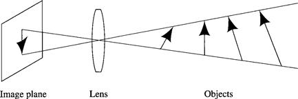
Figure 6.1 The Many-to-One Nature of the Imaging Process
The kinds of information to be extracted depend on the purposes and tasks of the agent. To navigate safely through a cluttered environment, an agent needs to know about the locations of objects, boundaries, and openings and about the surface properties of its path. To manipulate objects, it needs to know about their locations, sizes, shapes, compositions, and textures. For other purposes, it may need to know about their color and to be able to recognize them as belonging to certain classes. Based on how all of this information has changed over an observed time interval, an agent might need to be able to predict probable future changes. Extracting such information from one or more images is a tall order, and, as previously mentioned, I can only give a general overview of some of the techniques.
6.2 Steering an Automobile
In certain applications involving S-R agents, neural networks can be used to convert the image intensity matrix directly into actions. A prominent example is the ALVINN1 system for steering an automobile [Pomerleau 1991, Pomerleau 1993]. I discuss this system before dealing with more general processes for robot vision. The input to the network is derived from a low-resolution (30 × 32) television image. The TV camera is mounted on the automobile and looks at the road straight ahead. This image is sampled and produces a stream of 960-dimensional input vectors to the neural network. The network is shown in Figure 6.2.
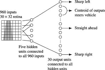
Figure 6.2 The ALVINN Network
The network has five hidden units in its first layer and 30 output units in the second layer; all are sigmoid units. The output units are arranged in a linear order and control the automobile’s steering angle. If a unit near the top of the array of output units has a higher output than most of the other units, the car is steered to the left; if a unit near the bottom of the array has a high output, the car is steered to the right. The “centroid” of the responses of all of the output units is computed, and the car’s steering angle is set at a corresponding value between hard left and hard right.
The system is trained by a modified “on-the-fly” training regime. A human driver drives the car, and his actual steering angles are taken as the correct labels for the corresponding inputs. The network is trained incrementally by backprop to produce the driver-specified steering angles in response to each visual pattern as it occurs in real time while driving. Training takes about five minutes of driving time.
This simple procedure has been augmented to avoid two potential problems. First, since the driver is usually driving well, the network would never get any experience with far-from-center vehicle positions and/or incorrect vehicle orientations. Also, on long, straight stretches of road, the network would be trained for a long time only to produce straight-ahead steering angles; this training would overwhelm earlier training involving following a curved road. We wouldn’t want to try to avoid these problems by instructing the driver to drive erratically occasionally, because the system would learn to mimic this erratic behavior.
Instead, each original image is shifted and rotated in software to create 14 additional images in which the vehicle appears to be situated differently relative to the road. Using a model that tells the system what steering angle ought to be used for each of these shifted images, given the driver-specified steering angle for the original image, the system constructs an additional 14 labeled training vectors to add to each of those encountered during ordinary driver training.
After training, ALVINN has successfully steered various testbed vehicles on unlined paved paths, jeep trails, lined city streets, and interstate highways. On highways, ALVINN has driven for 120 consecutive kilometers at speeds up to 100 km/hr.
6.3 Two Stages of Robot Vision
Although ALVINN’s performance is impressive, more sophisticated processing of higher-resolution images is required for many robot tasks. Since many robot tasks involve the need to know about objects in the scene, I focus my discussion on techniques relevant to finding out about objects. First, what is an object? In man-made environments such as the interiors of buildings, objects can be doorways, furniture, other agents, humans, walls, floors, and so on. In exterior natural environments, objects can be animals, plants, man-made structures, automobiles, roads, and so on. Man-made environments are usually easier for robot vision because most of the objects tend to have regular edges and surfaces.
Two computer vision techniques are useful for delineating the parts of images that relate to objects in the scene. One technique looks for “edges” in the image. An image edge is a part of the image across which the image intensity or some other property of the image changes abruptly. Another technique attempts to segment the image into regions. A region is a part of the image in which the image intensity or some other property of the image changes only gradually. Often, but not always, edges in the image and boundaries between regions in the image correspond to important object-related discontinuities in the scene that produced the image. Some examples of discontinuities are illustrated in Figure 6.3.2 Depending on illumination levels, surface properties, and camera angle, these discontinuities might all be represented by image edges or image region boundaries. Thus, extracting these image features is an important task for robot vision.

Figure 6.3 Scene Discontinuities
I divide my discussion of visual processing into two major stages, as shown in Figure 6.4. The image processing stage is concerned with transforming the original image into one that is more amenable to the scene analysis stage. Image processing involves various filtering operations that help reduce noise, accentuate edges, and find regions in the image. Scene analysis routines attempt to create from the processed image either an iconic or a feature-based description of the original scene—providing the task-specific information about it that the agent needs. My division of robot vision into these two stages is a simplification; actual robot vision programs often involve more stages, and usually the stages interact.
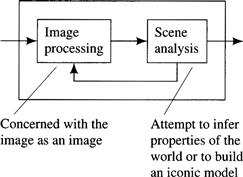
Figure 6.4 The Two Stages of Robot Vision
I will discuss the two stages in more detail later, but to give the general idea, consider the grid-space robot depicted in Figure 6.5. In view of the robot are three toy blocks with labels A, B, and C, a doorway, and a corner of the room. First, image processing eliminates spurious noise and accentuates the edges of objects and other discontinuities. Next, knowing that the world comprises objects and forms with rectilinear boundaries, the scene analysis component might produce an iconic representation of the visible world—similar, say, to the sort of models used in computer graphics. Typically, this iconic model is used to update the more comprehensive model of the environment stored in memory, and then actions appropriate to this presumed state of the environment are computed.

Figure 6.5 A Robot in a Room with Toy Blocks
Depending on the task, iconic models do not have to portray all the detail that a computer graphics model does. If the task at hand deals only with the toy blocks, then the location of the room corner and the doorway may be irrelevant. Suppose further that only the disposition of the blocks is important. Then the appropriate iconic model might be the list structure ((C B A FLOOR)), which is meant to represent that C is on top of B, which is on top of A, which is on the floor. If C were moved to the floor, the appropriate iconic model would be ((C FLOOR) (B A FLOOR)). (It could also be ((B A FLOOR) (C FLOOR)), but assuming that the relative horizontal locations of the blocks are also unimportant, the order of the first-level elements of the list structure need not have representational significance.) Since the last element of each component list is always FLOOR, we can shorten our lists by excluding this term.
For robots that do not use iconic models at all, scene analysis might alternatively convert the processed image directly into features appropriate to the task for which the robot is designed. If it is important, for example, to determine whether or not there is another block on top of the block labeled C, then an adequate description of the environment might include the value of a feature, say, CLEAR_C. This feature has value 1 if block C is clear; otherwise, it has value 0. (Here, I use mnenomic names for the features instead of the usual xi. We must remember though that the names are mnenomic just to help us; they are not mnenomic for the robot.) In this case, scene analysis has only to compute the value of this feature from the processed image. We see from these examples that the process of scene analysis is highly dependent on the design of the robot doing it and the tasks that it is to perform.
6.4 Image Processing
6.4.1 Averaging
We assume that the original image is represented as an m × n array, I(x, y), of numbers, called the image intensity array, that divides the image plane into cells called pixels. The numbers represent the light intensities at corresponding points in the image. Certain irregularities in the image can be smoothed by an averaging operation. This operation involves sliding an averaging window all over the image array. The averaging window is centered at each pixel, and the weighted sum of all the pixel numbers within the averaging window is computed. This sum then replaces the original value at that pixel. The sliding and summing operation is called convolution. If we want the resulting array to contain only binary numbers (say, 0 and 1), then the sum is compared with a threshold. Averaging tends to suppress isolated noise specks but also reduces the crispness of the image and loses small image components.
Convolution is an operation that derives from signal processing. It is often explained as a one-dimensional operation on waveforms (sliding over the time axis). If we slide or convolve a function w(t) over a signal, s(f), we get the averaged signal, s*(t):
![]()
I use the operator * to denote convolution.
In image processing, the two-dimensional, discrete version of convolution is
![]()
where I(x, y) is the original image array, and W(u, v) is the convolution weighting function. I assume that I(x, y) = 0 for x < 0 or x ≥ n and y < 0 or y ≥ m. (Thus, the convolution operation will have some “edge effects” near the boundaries of the image.)
Sometimes, the value of the weighting function W(x, y) is taken to be 1 over a rectangular range of x and y and zero outside of this range. The size of the rectangle determines the degree of smoothing, with larger rectangles achieving more smoothing. I show an example of what the averaging operation does for a binary image smoothed by a rectangular smoothing function and then thresholded in Figure 6.6. (In this figure, I assume that black pixels have a high intensity value and that white pixels have a low or zero intensity value. This convention may seem reversed, but it makes this illustration a bit simpler.) Notice that the smoothing operation thickens broad lines and eliminates thin lines and small details.
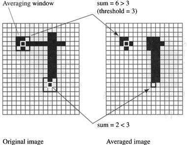
Figure 6.6 Elements of the Averaging Operation
A very common function used for smoothing is a Gaussian of two dimensions:
![]()
The surface described by this function is bell-shaped, as shown in Figure 6.7. (I have displaced the axes in this figure in order to display the Gaussian surface more clearly.) The standard deviation, ∑, of the Gaussian determines the “width” of the surface and, thus, the degree of smoothing. G(x, y) has a unit integral over x and y. Three Gaussian-smoothed versions of a grid-space scene containing blocks and a robot, using different smoothing factors, are shown along with the original image in Figure 6.8.3 (Discrete versions of image smoothing and filtering operations usually interpolate between discrete values to enhance performance.)
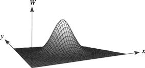
Figure 6.7 The Gaussian Smoothing Function
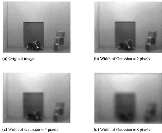
Figure 6.8 Image Smoothing with a Gaussian Filter
You will note that the sequence of images in Figure 6.8 is increasingly blurred. One way to think about this blurring is to imagine that the image intensity function I(x, y) represents an initial temperature field over a rectangular, heat-conducting plate. As time passes, heat diffuses isotropically on the plate causing high temperatures to blend with lower ones. According to this view, the sequence of images in Figure 6.8 represents temperature fields at later and later points of time. Koenderink [Koenderink 1984] has noted that convolving an image with a Gaussian with standard deviation ∑ is, in fact, equivalent to finding the solution to a diffusion equation at time proportional to ∑ when the initial condition is given by the image intensity field.
6.4.2 Edge Enhancement
As previously mentioned, computer vision techniques frequently involve extracting image edges. These edges are then used to convert the image to a line drawing of some sort. The outlines in the converted image can then be compared against prototypical (model) outlines characteristic of the sorts of objects that the scene might contain. One method of extracting outlines begins by enhancing boundaries or edges in the image. An edge is any boundary between parts of the image with markedly different values of some property, such as intensity. Such edges are often related to important object properties as illustrated in Figure 6.3.
I motivate my discussion by first considering images that are only “one-dimensional” in the sense that I(x, y) varies only along the x dimension, not along the y dimension. Then, I will generalize to the two-dimensional case. We can enhance intensity edges in one-dimensional images by convolving a vertically oriented, partly negative, partly positive window over the image. Such a window is shown in Figure 6.9. The window sum is zero over uniform parts of the image.
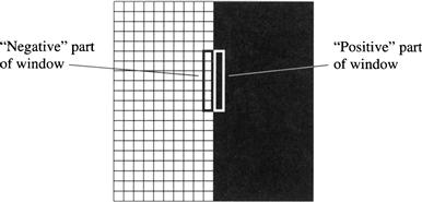
Figure 6.9 Edge Enhancement
If the window shown in Figure 6.9 is convolved in the x direction over an image, a peak will result at positions where an edge is aligned with the y direction. This operation is approximately like taking the first derivative, dI/dx, of the image intensity function with respect to x. An even more pronounced effect would occur if we were to take the second derivative of the image intensity. In that case, we would get a positive band on one side of the edge, crossing through zero at the edge, and a negative band on the other side of the edge. These effects, illustrated for one dimension, are shown in Figure 6.10, in which the intensity changes smoothly (and thus differentiably) instead of abruptly as in Figure 6.9. Of course, the steeper the change in image intensity, the narrower will be the peak in dI/dx. Edges in the image occur at places where d2I/dx2 = 0, that is, at the “zero-crossings” of the twice-differentiated image.
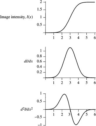
Figure 6.10 Taking Derivatives of Image Intensity
6.4.3 Combining Edge Enhancement with Averaging
Edge enhancement alone would tend to emphasize spurious noise elements of the image along with enhancing edges. To be less sensitive to noise, we can combine the two operations, first averaging and then edge enhancing. In the continuous, one-dimensional case, we use a one-dimensional Gaussian for smoothing. It is given by
![]()
where ∑ is the standard deviation, which is a measure of the width of the smoothing function. Smoothing with a Gaussian gives the filtered image
![]()
Subsequent edge enhancement yields
![]()
which is equivalent to I(x) * d2G(x)/dx2 because the order of differentiation and integration can be interchanged. That is, to combine smoothing with edge enhancement, we can convolve the one-dimensional image with the second derivative of a Gaussian curve instead of having to take the second derivative of a convolved image.
Moving now to two dimensions, we need a second-derivative-type operation that enhances edges of any orientation. The Laplacian is such an operation. The Laplacian of I(x, y) is defined as
![]()
If we want to combine edge enhancement with Gaussian smoothing in two dimensions, we can interchange the order of differentiation and convolution (as in the one-dimensional case), yielding
![]()
The Laplacian of the two-dimensional Gaussian function looks a little bit like an upside-down hat, as shown in Figure 6.11. (Again, I have translated the origin of the coordinate space.) It is often called a sombrero function. The width of the hat determines the degree of smoothing.

Figure 6.11 The Sombrero Function Used in Laplacian Filtering
The entire averaging/edge-finding operation, then, can be achieved by convolving the image with the sombrero function. This operation is called Laplacian filtering; it produces an image called the Laplacian filtered image. It has been remarked that early visual processing in the retinas of vertebrates seems to resemble Laplacian filtering. The zero-crossings of the Laplacian filtered image can then be used to create a rough outline drawing. The entire process, Laplacian filtering and zero-crossing marking, constitutes what is called the Marr-Hildreth operator [Marr & Hildreth 1980]. (The output of the Marr-Hildreth operator is a component of what Marr called the primal sketch.) I show the results of these operations on the image of the grid-space scene in Figure 6.12.4 Note that the Marr-Hildreth operator provides a reasonable basis for an outline sketch for those parts of the scene with simple boundaries. The more complex robot in front of the doorway, however, is not well delineated.
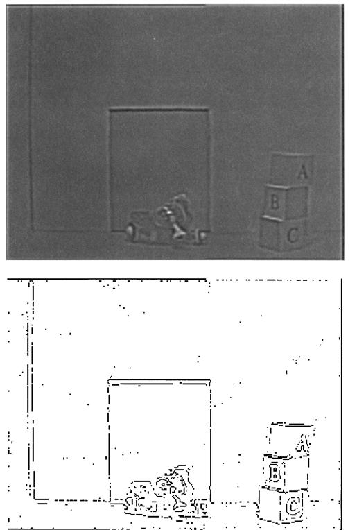
Figure 6.12 Laplacian Filtering and the Marr-Hildreth Operator (width of Laplacian = 1 pixel)
There are several other edge-enhancing and line-finding operations, some of which produce better results than does the easy-to-explain and popular Marr-Hildreth operator. Among the prominent ones are the Canny operator ([Canny 1986]), the Sobel operator (attributed to Irwin Sobel by [Pingle 1969]), the Hueckel operator ([Hueckel 1973]), and the Nalwa-Binford operator ([Nalwa & Binford 1986]). It should be noted that the Marr-Hildreth and other edge-enhancing operators label pixels as candidates that might be on an image edge or line. The candidate pixels must then be linked to form lines or other simple curves.
6.4.4 Region Finding
Another method for processing an image attempts to find “regions” in the image within which intensity or some other property, such as texture, does not change abruptly. In a sense, finding regions is a process that is dual to finding outlines; both techniques segment the image into, we hope, scene-relevant portions. But since finding outlines and finding regions are both subject to idiosyncrasies due to noise, the two techniques are often used to complement each other.
First, I must define what is meant by a region of the image. A region is a set of connected pixels satisfying two main properties:
1. A region is homogeneous. Examples of commonly used homogeneity properties are as follows:
(a) The difference in intensity values of pixels in the region is no more than some ε.
(b) A polynomial surface of degree k (for some low, preassigned value of k) can be fitted to the intensity values of pixels in the region with largest error (between the surface and an intensity value in the region) less than ε.
2. For no two adjacent regions is it the case that the union of all the pixels in these two regions satisfies the homogeneity property.
Usually, there is more than one possible partition of an image into regions, but, often, each region corresponds to a world object or to a meaningful part of one.
As with edge enhancement and line finding, there are many different techniques for segmenting a scene into regions. I will describe one of these, called the split-and-merge method [Horowitz & Pavlidis 1976]. In a version that is rather easy to describe, the algorithm begins with just one candidate region, namely, the whole image. For ease of illustration, let’s assume the image is square and consists of a 2l × 2l array of pixels. Obviously, this candidate region will not meet the definition of a region because the set of all the pixels in an image will not satisfy the homogeneity property (except for an image of uniform intensity). For all candidate regions that do not satisfy the homogeneity property, those candidate regions are each split into four equal-sized candidate regions. These splits continue until no more splits need be made. In Figure 6.13, I illustrate the splitting process for an artificial 8 × 8 image using a homogeneity property in which intensities may not vary by more than 1 unit. After no more splits can be made, adjacent candidate regions are merged if their pixels satisfy the homogeneity property. Merges can be done in different orders—resulting in different final regions. In fact, some merges could have been performed before the splitting process finished. To simplify my illustration of the process in Figure 6.13, all of the merges take place in the last step.
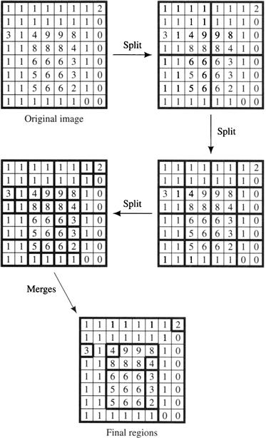
Figure 6.13 Splitting and Merging Candidate Regions
I used the low-resolution image of Figure 6.13 to illustrate the region-finding process. I show results for a higher-resolution image in Figure 6.14. Just as in Figure 6.13, we see some small regions and many irregularities in the region boundaries. The regions found by the split-merge algorithm can often be “cleaned up” by eliminating very small regions (some of which are transitions between larger regions), straightening bounding lines, and taking into account the known shapes of objects likely to be in the scene. Intensity gradients along the wall of the grid-world scene produce many regions in the image of Figure 6.14.
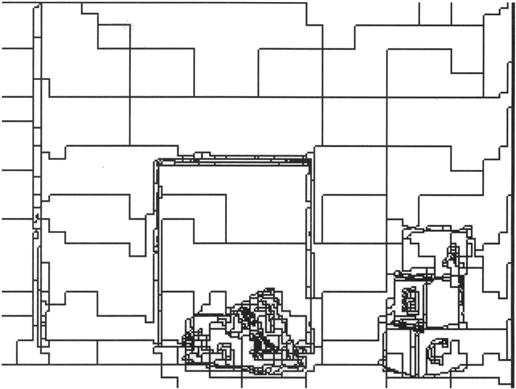
Figure 6.14 Regions Found by Split Merge for a Grid-World Scene
Recall that in my discussion of image smoothing with a Gaussian, I mentioned that the process was related to isotropic heat diffusion. Perona and Malik [Perona & Malik 1990] have proposed a process of anisotropic diffusion that can be used to create regions. The process encourages smoothing in directions of small intensity change and resists smoothing in directions of large intensity change. As described by [Nalwa 1993, p. 96], the result is “the formation of uniform-intensity regions that have boundaries across which the intensity gradient is high.”
6.4.5 Using Image Attributes Other Than Intensity
Edge enhancement and region finding can be based on image attributes other than the homogeneity of image intensity. Visual texture is one such attribute. The surface reflectivity of many objects in the world has fine-grained variation, which we call visual texture. Examples are a field of grass, a section of carpet, foliage in trees, the fur of animals, and so on. These reflectivity variations in objects cause similar fine-grained structure in image intensity.
Computer vision researchers have identified many varieties of texture and have developed various tools for analyzing texture. Among these are structural and statistical methods. The methods are applied either to classify parts of the image as having textures of a certain sort or to segment the image into regions such that each region has its own special texture. The structural methods attempt to represent regions in the image by a tessellation of primitive “texels”—small shapes comprising black and white parts. (See [Ballard & Brown 1982, Ch. 6] for a thorough discussion.)
Statistical methods are based on the idea that image texture is best described by a probability distribution for the intensity values over regions of the image. As a rough example, an image of a grassy field in which the blades of grass are oriented vertically in the image would have a probability distribution that peaks for thin, vertically oriented regions of high intensity, separated by regions of low intensity. Recent work by Zhu and colleagues [Zhu, Wu, & Mumford 1998] involves estimating these probability distributions for various types of visual textures. Once the distributions are known, they can be used to classify textures and to segment images based on texture.
In addition to texture, there are other attributes of the image that might be used. If we had a direct way to measure the range from the camera to objects in the scene (say, with a laser range finder), we could produce a “range image” (where each pixel value represents the distance from the corresponding point in the scene to the camera) and look for abrupt range differences. Motion and color are other properties that might be sensed or computed and subjected to image processing operations.
6.5 Scene Analysis
After the image has been processed by techniques such as those just discussed, we can attempt to extract from it the needed information about the scene. This phase of computer vision is called scene analysis. Since the scene-to-image transformation is many-to-one, the scene analysis phase requires either additional images or general information about the kinds of scenes to be encountered (or both). I will discuss the use of additional images later when I describe stereo vision; here I mention various methods in which knowledge about the scene can be used to extract information about it.
The required extra knowledge can be very general (such as the surface reflectivity properties of objects) or quite specific (such as the scene is likely to contain some stacked boxes near a doorway). It can also be explicit or implicit. For example, a line-finding algorithm might have implicit knowledge about what constitutes a line built into its operation. Between these extremes are other pieces of information about the scene, such as camera location, locations of illumination sources, and whether the scene is indoors in an office building or outdoors. My discussion below samples some points along these spectra. Again, please see computer vision textbooks for detailed treatments.
Knowledge of surface reflectivity characteristics and shading of intensity in the image can often be used to give information about the shape of smooth objects in the scene. Specifically, we can use image shading to help compute surface normals of objects. Methods for inferring shape from shading have been developed by Horn and colleagues (see [Horn 1986] for descriptions). The fact that textural elements as represented in the image are perspective projections of elements in the scene also facilitates shape and qualitative depth recovery from texture.
As already mentioned, sometimes an iconic model of the scene is desired, and sometimes certain features of the scene suffice. Iconic scene analysis usually attempts to build a model of the scene or of parts of the scene. Feature-based scene analysis extracts features of the scene needed by the task at hand. So-called task-oriented or purposive vision (see, for example, [Ballard 1991, Aloimonos 1993]) typically employs feature-based scene analysis.
6.5.1 Interpreting Lines and Curves in the Image
For scenes that are known to contain rectilinear objects (such as the scenes confronted inside of buildings and scenes in grid-space world), an important step in scene analysis is to postulate lines in the image (which later can be associated with key components of the scene). Lines in the image can be created by various techniques that fit segments of straight lines to edges or to boundaries of regions. For scenes with curved objects, curves in the image can be created by attempting to fit conic sections (such as ellipses, parabolas, and hyperbolas) to the primal sketch or to boundaries of regions. (See, for example, [Nalwa & Pauchon 1987].) These fitting operations, followed by various techniques for eliminating small lines and joining line and curve segments at their extremes, convert the image into a line drawing, ready for further interpretation.
Various strategies exist for associating scene properties with the components of a line drawing. Such an association is called interpreting the line drawing. By way of example, I mention here one strategy for interpreting a line drawing if the scene is known to contain only planar surfaces such that no more than three surfaces intersect in a point. (Such combinations of surfaces are called trihedral vertex polyhedra.) I show a typical example of such a scene in Figure 6.15. Illustrated there is an interior scene with bounding walls, floor, and ceiling, with a cube on the floor. For such scenes, there are only three kinds of ways in which two planes can intersect in a scene edge. One kind of edge is formed by two planes, with one of them occluding the other (that is, only one of the planes is visible in the scene). Such an edge is called an occlude. The occludes are labeled in Figure 6.15 with arrows (→), with the arrowhead pointing along the edge such that the surface doing the occluding is to the right of the arrow. Alternatively, two planes can intersect such that both planes are visible in the scene. In one such intersection, called a blade, the two surfaces form a convex edge. These edges are labeled with pluses (+). In another type of intersection, called a fold, the edge is concave. These edges are labeled with minuses (–).

Figure 6.15 A Room Scene
Suppose an image is captured from such a scene and suppose that the image can be converted into a line drawing—much like the one shown in Figure 6.15. Can we label the lines in the image in such a way that they accurately describe the types of edges in the scene? Under certain conditions, we can. First the image of the scene must be taken from a general viewpoint, one in which no two edges in the scene line up to produce just one line in the image. The method for attempting to label lines in the image is based on the fact that (under our assumption about trihedral vertex polyhedra) there can only be certain kinds of labelings of junctions of lines in the image. The different kinds of labelings are shown in Figure 6.16. Even though there are many more ways to label the lines at image junctions, these are the only labelings possible for our polyhedral scenes.

Line-labeling scene analysis proceeds by first labeling all of the junctions in the image as V, W, Y, or T junctions according to the shape of the junctions in the image. I have done that for the image of our room scene in Figure 6.17. (Note that there are no T junctions in this image.) Next, we attempt to assign +, –, or → labels to the lines in the image. But we must do that in one of the ways illustrated in Figure 6.16. Also, an image line that connects two junctions must have a consistent labeling. These constraints often (but not always) force a unique labeling. If there is no consistent labeling, then there must have been some error in converting the image into a line drawing, or the scene must not have been one of trihedral polyhedra. The problem of assigning labels to the image lines, subject to these constraints, is an instance of what in AI is called a constraint satisfaction problem. I will discuss methods for solving this general class of problem later, but in the meantime, you might experiment with methods for coming up with a consistent labeling for the image of Figure 6.17. (Of course, a labeling of the image corresponding to the labeled scene in Figure 6.15 is one such consistent labeling, but the scene was stipulated to have those labels. Can you think of an automatic way to find a consistent labeling for the image lines?)

Figure 6.17 Labeling Image Junctions According to Type
Scene analysis techniques that label junctions and lines in images of trihedral vertex polyhedra began with [Guzman 1968, Huffman 1971, Clowes 1971] and were extended by [Waltz 1975] and others. Some success has also been achieved at performing similar analyses for scenes containing nonplanar surfaces. For a more complete exposition (with citations) of work on interpreting line drawings, see [Nalwa 1993, Ch. 4].
Interpretation of the lines and curves of a line drawing yields a great deal of useful information about a scene. For example, a robot could predict that heading toward a vertically oriented fold (a concave edge in the scene) would eventually land it in a corner. Navigating around polyhedral obstacles could be performed by skirting vertically oriented blades (convex edges). With sufficient general knowledge about the class of scenes, either the needed features or iconic models can be obtained directly from an interpreted line drawing.
6.5.2 Model-Based Vision
Progressing further along the spectrum of using increasing knowledge about the scene, I now turn to the use of models of objects that might appear in the scene. If, for example, we knew that the scene consisted of industrial parts and components used in robot assembly, then geometric models of the shapes of these parts could be used to help interpret images. I give a brief overview of some of the methods used in model-based vision; see [Binford 1982, Grimson 1990, Shirai 1987] for further reading.
Just as lines and curves can be fitted to boundary sections of regions in the image, so can perspective projections of models and parts of models. If, for example, we knew that the scene contained a parallelepiped (as does the scene in Figure 6.15), we could attempt to fit a projection of a parallelepiped to components of an image of this scene. The parallelepiped would have parameters specifying its size, position, and orientation. These would be adjusted until a set of parameters is found that allowed a good fit to an appropriate set of lines in the image.
Researchers have also used generalized cylinders [Binford 1987] as building blocks for model construction. A generalized cylinder is shown in Figure 6.18. Each cylinder has nine parameters as shown in the figure. An example rough scene reconstruction of a human figure is shown in Figure 6.19. The method can be adapted to hierarchical representations, because each cylinder in the model can be articulated into a set of smaller cylinders that more accurately represent the figure. Representing objects in a scene by a hierarchy of generalized cylinders is, as Nalwa says, “easier said than done” [Nalwa 1993, p. 293], but the method has been used for certain object-recognition applications [Brooks 1981]. For more discussion on the use of models in representing three-dimensional structures, see [Ballard & Brown 1982, Ch. 9].
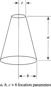
Figure 6.18 A Generalized Cylinder

Figure 6.19 A Scene Model Using Generalized Cylinders
Using a variety of model components, model fitting can be employed until either an iconic model of the entire scene is produced or sufficient information about the scene is obtained to allow the extraction of features needed for the task at hand. Model-based methods can test their accuracy by comparing the actual image with a simulated image constructed from the iconic model produced by scene analysis. The simulated image must be rendered from the model using parameters similar to those used by the imaging process (camera angle, etc.). To do so requires good models of illumination, surface reflectance characteristics, and all of the other aspects of the rendering processes of computer graphics.
6.6 Stereo Vision and Depth Information
Under perspective projection, a large, distant object might produce the same image as does a similar but smaller and closer one. Thus, the estimation of the distance to objects from single images is problematical. Depth information can be obtained using stereo vision, which is based on triangulation calculations using two (or more) images.
Before discussing stereo vision, however, I point out that under some circumstances, and with appropriate prior knowledge, some depth information can be extracted from a single image. For example, the analysis of texture in the image (taking into account the perspective transformation of scene texture) can indicate that some elements in the scene are closer than are others. Even more precise depth information can be obtained from single images in certain situations. In an office scene, for example, if we know that a perceived object is on the floor, and if we know the camera height above the (same) floor, then, using the angle from the camera lens center to the appropriate point on the image, we can calculate the distance to the object. An example of such a calculation is shown in Figure 6.20. (The angle α can be calculated in terms of the camera focal length and image dimensions.) Similar calculations can be used to calculate distances to doorways, sizes of objects, and so on.

Figure 6.20 Depth Calculation from a Single Image
Stereo vision also uses triangulation. The basic idea is very simple. Consider the two-dimensional setup shown in Figure 6.21. There we have two lenses whose centers are separated by a baseline, b. The image points of a scene point, at distance d, created by these lenses are as illustrated. The angles of these image points from the lens centers can then be used to calculate d, as shown. For given precision in the measurements of angles and baseline, higher accuracies are obtained for larger baselines and smaller object distances. Figure 6.21 oversimplifies the situation somewhat in that the optical axes are parallel, the image planes are coplanar, and the scene point is in the same plane as that formed by the two parallel optical axes. When these conditions are generalized, the geometry is more complex, but the general idea of triangulation is the same. (In animals and in some robots, the optical axes can be rotated to point at an object of interest in the scene.)

Figure 6.21 Triangulation in Stereo Vision
The main complication in stereo vision, however, is not the triangulation calculations. In scenes containing more than one point (the usual case!), it must be established which pair of points in the two images correspond to the same scene point (in order to calculate the distance to that scene point). Put another way, for any scene point whose image falls on a given pixel in one image, we must be able to identify a corresponding pixel in the other image. Doing so is known as the correspondence problem. Space does not permit detailed discussion of techniques for dealing with the correspondence problem, but I will make a few observations.
First, given a pixel in one image, geometric analysis reveals that we need only search along one dimension (rather than two) for a corresponding pixel in the other image. This one dimension is called an epipolar line. One-dimensional searches can be implemented by cross-correlation of two image intensity profiles along corresponding epipolar lines. Second, in many applications, we do not have to find correspondences between individual pairs of image points but can do so between pairs of larger image components, such as lines.5 Scene analysis of each image can provide clues as to which pairs of lines correspond. For an excellent review of computational methods in stereo vision, see [Nalwa 1993, Ch. 7].
6.7 Additional Readings and Discussion
The team that developed ALVINN continues to develop other autonomous driving systems, some of which use techniques related to those I discussed in this chapter ([Thorpe, et al. 1992]). In a related effort, [Hebert, et al. 1997] describes mobility software for an autonomous vehicle driving in open terrain using both stereo and infrared sensors.
Although there are applications in which a three-dimensional model of an entire scene is required from a computer vision system, usually robots require only information sufficient to guide action. Reacting to early work in vision directed at computing complete scene models, some researchers have concentrated on what they consider to be the more relevant task of purposive vision. [Horswill 1993] gives an interesting example of a simple, task-oriented robotic vision system. These task-oriented systems often suffice for robust mobile robot navigation. See also [Churchland, Ramachandran, & Sejnowski 1994].
Much about the process of visual perception has been learned by studying the psychology and neurophysiology of human and animal vision. [Gibson 1950, Gibson 1979] studied, among other phenomena, how the changing visual field informed a moving subject about its surroundings. [Julesz 1971] discovered that humans can exploit discontinuities in the statistics of random dots to perceive depth. [Marr & Poggio 1979] developed a plausible neural model of stereo vision.
Experiments with frogs [Letvinn, et al. 1959] revealed that their visual system notices only changes in overall illumination (such as would be caused by the shadow of a large approaching animal) and rapid movement of small, dark objects (such as flies). Experiments with monkeys [Hubel & Wiesel 1968] revealed that neurons in their visual cortex were excited by short, oriented line segments in their visual field. Experiments with horseshoe crabs revealed that adjacent neurons in their visual system inhibit each other (lateral inhibition), achieving an effect much like what later came to be known as Laplacian filtering [Reichardt 1965]. For more on biological vision, see [Marr 1982, Hubel 1988].
[Bhanu & Lee 1994] employed genetic techniques for image segmentation.
The major computer vision conferences are the International Conference on Computer Vision (ICCV), the European Conference on Computer Vision (ECCV), and Computer Vision and Pattern Recognition (CVPR). The International Journal of Computer Vision is a leading journal.
Textbooks on computer vision include [Nalwa 1995, Horn 1986, Ballard & Brown 1982, Jain, Kasturi, & Schunck 1995, Faugeras 1993]. [Fischler & Firschein 1987] is a collection of some of the important papers. A book devoted to outdoor scenes is [Strat 1992]. [Gregory 1966] is a popular account of how we see.
Exercises
6.1 You are to design a visual system for detecting small black objects against a light background. Assume that the image of one of these objects is a square that is 5 pixels wide. Your system is to be used to create a Boolean feature that has value 1 whenever a single such image appears anywhere in a 100 × 100 image array and has value 0 for any other image. Describe how you would design such a system, first using a neural network (with one hidden layer) and second, using convolution with a specially designed weighting function.
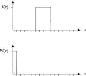
6.2 A one-dimensional image function, I(x), and a one-dimensional weighting function, W(x), are shown below. Draw a plot of I(x) * W(x).
6.3 A very simple edge finder (the so-called Roberts cross) computes an image I*(x, y) from an image I(x, y) according to the following definition:
![]()
where Δ is a one-pixel offset, and the positive root is taken. Use differential calculus to approximate this definition for small pixel sizes, and then use your approximation to compute I*(x, y) when I(x, y) is given in polar coordinates by
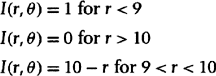
Assume a circular image field of radius 20. (Note: Expressing the image in polar coordinates is a hint that will be useful toward the end of your solution!) A rough sketch of the image intensity is shown here:

6.4 Copy the following drawing, and label the lines using the vertex classes and line labels discussed in Section 6.5.1. If there is more than one consistent labeling, show as many as you can think of, and describe a physical interpretation of each.

6.5 Can you find a consistent labeling for the lines in the image of the famous impossible figure called the Penrose triangle shown here? Assume the figure is suspended in empty space. Discuss the relationship between what might be called “local consistency” and “global consistency.”

1 Autonomous Land Vehicle In a Neural Network.
2 Adapted from [Nalwa 1993, p. 77].
3 I thank Charles Richards for creating the images and programming the image processing operations illustrated in this chapter.
4 In calculating the image of Figure 6.12,1 used “band” crossings instead of zero-crossings. The image intensity had to cross a band around zero in order to be displayed.
5 Or we can find correspondences between the image points where lines intersect.