
10
Planning, Acting, and Learning
Now that we have explored several techniques for finding paths in graphs, it is time to show how these methods can be used by agents in realistic settings. I first revisit the assumptions made when I first considered graph-search planning methods in Chapter 7 and propose an agent architecture that tolerates these idealized assumptions. Next, I show how some of the search methods can be modified to lessen their time and space requirements—thus making them more usable in the proposed architecture. Finally, I show how heuristic functions and models of actions can be learned.
10.1 The Sense/Plan/Act Cycle
As mentioned in Chapter 7, the efficacy of search-based planning methods depends on several strong assumptions. Often, these assumptions are not met because
1. Perceptual processes might not always provide the necessary information about the state of the environment (because they are noisy or are insensitive to important properties). When two different environmental situations evoke the same sensory input, we have what is called perceptual aliasing.
2. Actions might not always have their modeled effects (because the models are not precise enough or because the effector system occasionally makes errors in executing actions).
3. There may be other physical processes in the world or other agents (as there might be, for example, in games with adversaries). These processes might change the world in ways that would interfere with the agent’s actions.
4. The existence of external effects causes another problem: during the time that it takes to construct a plan, the world may change in such a way that the plan is no longer relevant. This difficulty makes it pointless for an agent to spend too much time planning.
5. The agent might be required to act before it can complete a search to a goal state.
6. Even if the agent had sufficient time, its computational memory resources might not permit search to a goal state.
There are two main approaches for dealing with these difficulties while preserving the main features of search-based planning. In one, probabilistic methods are used to formalize perceptual, environmental, and effector uncertainties. In the other, we attempt to work around the difficulties with various additional assumptions and approximations.
A formal way of confronting the fact that actions have uncertain effects is to assume that for every action executable in a certain state, the resulting state is given by a known probability distribution. Finding appropriate actions under such circumstances is called a Markov decision problem (MDP) [Puterman 1994]. Dealing with the additional problem of imperfect perception can be formalized by assuming that the agent’s sensory apparatus provides a probability distribution over the set of states that it might be in. Finding actions then is called a partially observable Markov decision problem (POMDP) [Lovejoy 1991, Monahan 1982, Cassandra, Kaelbling, & Littman 1994]. Discussing MDPs and POMDPs is beyond the scope of this book, but I touch on related techniques in Chapter 20 after my treatment of probabilistic inference.
Instead of pursuing the formal, probability-based methods here, I propose an architecture, called the sense/plan/act architecture, that gets around some of the aforementioned complications in many applications. The rationale for this architecture is that even if actions occasionally produce unanticipated effects and even if the agent sometimes cannot decide which world state it is in, these difficulties can be adequately dealt with by ensuring that the agent gets continuous feedback from its environment while it is executing its plan.
One way to ensure continuous feedback is to plan a sequence of actions, execute just the first action in this sequence, sense the resulting environmental situation, recalculate the start node, and then repeat the process. Agents that select actions in this manner are said to be sense/plan/act agents. For this method to be effective, however, the time taken to compute a plan must be less than the time allowed for each action. In Figure 10.1, I show an architecture for a sense/plan/act agent. In benign environments (those tolerant of a few missteps), errors in sensing and acting “average out” over a sequence of sense/plan/act cycles.
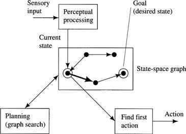
Figure 10.1 An Architecture for a Sense/Plan/Act Agent
Environmental feedback in the sense/plan/act cycle allows resolution of some of the perceptual, environmental, and effector uncertainties. For feedback to be effective, however, we must assume that, on the average, sensing and acting are accurate. In many applications, this assumption is realistic. After all, it is the agent designer’s task to provide sensory, perceptual, and effector modalities adequate to the task requirements. Often, the agent can enhance perceptual accuracy by comparing immediate sensory data with a stored model of the unfolding situation. (Recall that we saw a simple example of such filtering in the illustrative blackboard system of Chapter 5.)
10.2 Approximate Search
I next treat modifications to the search process that address the problem of limited computational and/or time resources at the price of producing plans that might be suboptimal or that might not always reliably lead to a goal state. Application of these techniques can then be incorporated in a sense/plan/act cycle even if the plan is not optimal (nor even correct). Qualitatively, so long as the first action has a tendency (on the average) to shorten the distance to the goal, multiple iterations of the sense/plan/act cycle will eventually achieve the goal.
As mentioned in the last chapter, relaxing the requirement of producing optimal plans often reduces the computational cost of finding a plan. This reduction can be done in either of two ways. First, we could search for a complete path to a goal node without requiring that it be optimal. Or we could search for a partial path that does not take us all the way to a goal node. An A*-type search can be used in both methods. In the first, we use a nonadmissible heuristic function, and in the second, we quit searching before reaching the goal—using either an admissible or nonadmissible heuristic function. Discontinuing search before reaching the goal is an example of an anytime algorithm [Dean & Boddy 1988, Horvitz 1987]. Anytime algorithms are ones that can be stopped at any time; the quality of the result generally improves with longer running times. In the next few subsections, we elaborate on these and other approximate search methods.
10.2.1 Island-Driven Search
In island-driven search, heuristic knowledge from the problem domain is used to establish a sequence of “island nodes” in the search space through which it is suspected that good paths pass. For example, in planning routes through difficult terrain, such islands might correspond to mountain passes. Suppose n0 is the start node, ng is the goal node, and (n1, n2, …, nk) is a sequence of such islands. We initiate a heuristic search with no as the start node and with n1 as the goal node (using a heuristic function appropriate for that goal). When the search finds a path to n1, we start another search with n1 as the start node and n2 as the goal node, and so on until we find a path to ng. I show a schematic illustration of island-driven search in Figure 10.2.

Figure 10.2 An Island-Driven Search
10.2.2 Hierarchical Search
Hierarchical search is much like island-driven search except that we do not have an explicit set of islands. We assume that we have certain “macro-operators” that can take large steps in an implicit search space of islands. A start island (near the start node) and these macro-operators form an implicit “metalevel” supergraph of islands. We search the supergraph first, with a metalevel search, until we produce a path of macro-operators that takes us from a node near the base-level start node to a node near the base-level goal node. If the macro-operators are already defined in terms of a sequence of base-level operators, the macro-operators are expanded into a path of base-level operators, and this path is then connected, by base-level searches, to the start and goal nodes. If the macro-operators are not defined in terms of the base-level operators, we must do base-level searches along the path of island nodes found by the metalevel search. The latter possibility is illustrated schematically in Figure 10.3.
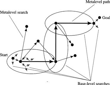
Figure 10.3 A Hierarchical Search
As an example of hierarchical planning, consider the grid-space robot task of pushing a block to a given goal location. The situation is as illustrated in Figure 10.4. A pushable block is located in one of the cells as shown. The robot’s goal is to push the block to the cell marked with a G. I assume that the robot can sense its eight surrounding cells and can determine whether an occupied surrounding cell contains an immovable barrier or a pushable block. As in Chapter 2, I assume that the robot can move in its column or row into an adjacent free cell or into an adjacent cell containing a pushable block, in which case the block moves one cell forward also (unless such motion is blocked by an immovable barrier).

Figure 10.4 Pushing a Block
Suppose the robot has an iconic model of its world, represented by an array similar to the cell array shown in Figure 10.4. Then, the robot could first make a metalevel plan of what the block’s moves should be—assuming the block can move in the same way that the robot can move. The result of such a plan is shown by the gray arrow in Figure 10.4. Each step of the block’s motion is then expanded into a base-level plan. The first one of the block’s moves requires the robot to plan a path to a cell adjacent to the block and on the opposite side of the next target location for the block. The result of that episode of base-level planning is shown by a dark arrow in Figure 10.4. Subsequent base-level planning is trivial until the block must change direction. Then, the robot must plan a path to a cell opposite the block’s direction of motion, and so on. The base-level plans to accomplish these changes in direction are also shown in Figure 10.4.1
In hierarchical planning, if there is likelihood of environmental changes during plan execution, it may be wise to expand only the first few steps of the metalevel plan. Expanding just the first metalevel step gives a base-level action to execute, after which environmental feedback can be used to develop an updated metalevel plan.
10.2.3 Limited-Horizon Search
In some problems, it is computationally infeasible for any search method to find a path to the goal. In others, an action must be selected within a time limit that does not permit search all the way to a goal. In these, it may be useful to use the amount of time or computation available to find a path to a node thought to be on a good path to the goal even if that node is not a goal node itself. This substitute for a goal, let’s call it node n*, is the one having the smallest value of ![]() among the nodes on the search frontier when search must be terminated.
among the nodes on the search frontier when search must be terminated.
Suppose the time available for search before an action must be selected allows search to a depth d. That is, all paths of length d or less can be searched. Nodes at that depth, denoted by H, will be called horizon nodes. Then our search process will be to search to depth d and then select
![]()
as a surrogate for a goal node. I call this method limited-horizon search. [Korf 1990] studied this technique and calls it minimin search.2 A sense/plan/act system would then take the first action on the path to n*, sense the resulting state, and iterate by searching again and so on. We can expect that this first action toward a node having optimal heuristic merit has a good chance of being on a path to a goal. And, often an agent does not need to search all the way to a goal anyway; because of uncertainties, distant search may be irrelevant and provide no better information than does the heuristic function applied at the search horizon.
Limited-horizon search can be efficiently performed by a depth-first process to depth d. The use of a monotone ![]() function to evaluate nodes permits great reductions in search effort. As soon as the first node, say, n1, on the search horizon is reached, we can terminate search below any other node, n, with
function to evaluate nodes permits great reductions in search effort. As soon as the first node, say, n1, on the search horizon is reached, we can terminate search below any other node, n, with ![]() . Node n cannot possibly have a descendant with an
. Node n cannot possibly have a descendant with an ![]() value less than
value less than ![]() , so there is no point in searching below it. (Under the monotone assumption, the
, so there is no point in searching below it. (Under the monotone assumption, the ![]() values of nodes along any path in the search tree are monotone nondecreasing.)
values of nodes along any path in the search tree are monotone nondecreasing.) ![]() is called an alpha cut-off value, and the process of terminating search below node n is an instance of a search process called branch and bound. Furthermore, whenever some other search-horizon node, say, n2, is reached such that
is called an alpha cut-off value, and the process of terminating search below node n is an instance of a search process called branch and bound. Furthermore, whenever some other search-horizon node, say, n2, is reached such that ![]() , the alpha cut-off value can be lowered to
, the alpha cut-off value can be lowered to ![]() , which relaxes the condition for cut-offs. Alpha cut-off values can be lowered in this way whenever horizon nodes are reached having
, which relaxes the condition for cut-offs. Alpha cut-off values can be lowered in this way whenever horizon nodes are reached having ![]() values smaller than the current alpha cut-off value. [Korf 1990] compares limited-horizon search with various other similar methods, including IDA* and versions of A* subject to limited time.
values smaller than the current alpha cut-off value. [Korf 1990] compares limited-horizon search with various other similar methods, including IDA* and versions of A* subject to limited time.
An extreme form of limited-horizon search uses a depth bound of 1. The immediate successors of the start node are evaluated, and the action leading to the successor with the lowest value of ![]() is executed. These
is executed. These ![]() values are analogous to the values of potential functions that I discussed in connection with robot navigation in Chapter 5, and, indeed, a potential function might well be an appropriate choice for
values are analogous to the values of potential functions that I discussed in connection with robot navigation in Chapter 5, and, indeed, a potential function might well be an appropriate choice for ![]() in robot navigation problems.
in robot navigation problems.
Formally, let σ(n0, a) be the description of the state the agent expects to reach by taking action a at node n0. Applying the operator corresponding to action a at node n0 produces that state description. Our policy for selecting an action at node no, then, is given by
![]()
where c(a) is the cost of the action. I will use an equation similar to this later when I discuss methods for learning ![]() .
.
10.2.4 Cycles
In all of these cases where there are uncertainties and where an agent relies on approximate plans, use of the sense/plan/act cycle may produce repetitive cycles of behavior. That is, an agent may return to a previously visited environmental state and repeat the action it took there. Getting stuck in such cycles, of course, means that the agent will never reach a goal state. Korf has proposed a plan-execution algorithm called Real-time A* (RTA*) that builds an explicit graph of all states actually visited and adjusts the ĥ values of the nodes in this graph in a way that biases against taking actions leading to states previously visited [Korf 1990].
10.2.5 Building Reactive Procedures
As mentioned at the beginning of Chapter 7, in a reactive machine, the designer has precalculated the appropriate goal-achieving action for every possible situation. Storing actions indexed to environmental states may require large amounts of memory. On the other hand, reactive agents can usually act more quickly than can planning agents. In some cases, it may be advantageous to precompute (compile) some frequently used plans offline and store them as reactive routines that produce appropriate actions quickly online.
For example, offline search could compute a spanning tree rooted at the goal of the state-space graph and containing paths from all (or, at least, many) of the nodes in the state space. A spanning tree can be produced by searching “backward” from the goal. For example, a spanning tree for achieving the goal block A is on block B is on block C is shown in Figure 10.5. It shows paths to the goal from all of the other nodes.
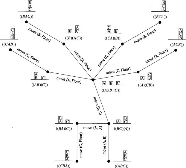
Figure 10.5 A Spanning Tree for a Block-Stacking Problem
Spanning trees and partial spanning trees can easily be converted to T-R programs, which are completely reactive. If a reactive program specifies an action for every possible state, it is called a universal plan [Schoppers 1987] or an action policy. I discuss action policies and methods for learning action policies toward the end of this chapter. Even if an action taken in a given state does not always result in the anticipated next state, the reactive machine is prepared to deal with whichever state does result.
10.3 Learning Heuristic Functions
Continuous feedback from the environment is one way to reduce uncertainties and to compensate for an agent’s lack of knowledge about the effects of its actions. Also, useful information can be extracted both from the experience of searching and from the experience of acting in the world. I will discuss various ways in which an agent can learn to plan and to act more effectively.
10.3.1 Explicit Graphs
If the agent does not have a good heuristic function to estimate the cost to the goal, it is sometimes possible to learn such a function. I first explain a very simple learning procedure appropriate for the case in which it is possible to store an explicit list of all of the possible nodes.3
I assume first that the agent has a good model of the effects of its actions and that it also knows the costs of moving from any node to its successor nodes. We begin the learning process by initializing the ![]() function to be identically 0 for all nodes, and then we start an A* search. After expanding node ni to produce successors
function to be identically 0 for all nodes, and then we start an A* search. After expanding node ni to produce successors ![]() , we modify
, we modify ![]() as follows:
as follows:
![]()
where c(ni, nj) is the cost of moving from ni to nj. The ![]() values can be stored in a table of nodes (because there is a manageably small number of them). I assume also that if a goal node, say, ng, is generated, we know that
values can be stored in a table of nodes (because there is a manageably small number of them). I assume also that if a goal node, say, ng, is generated, we know that ![]() . Although this learning process does not help us reach a goal the first time we search any faster than would uniform-cost search, subsequent searches to the same goal (from possibly different starting states) will be accelerated by using the learned
. Although this learning process does not help us reach a goal the first time we search any faster than would uniform-cost search, subsequent searches to the same goal (from possibly different starting states) will be accelerated by using the learned ![]() function. After several searches, better and better estimates of the true h function will gradually propagate backward from goal nodes. (The learning algorithm LRTA* uses this same update rule for
function. After several searches, better and better estimates of the true h function will gradually propagate backward from goal nodes. (The learning algorithm LRTA* uses this same update rule for ![]() [Korf 1990].)
[Korf 1990].)
If the agent does not have a model of the effects of its actions, it can learn them and also learn an ![]() function at the same time by a similar process, although the learning will have to take place in the actual world rather than in a state-space model. (Of course, such learning could be hazardous!) I assume that the agent has some means to distinguish the states that it actually visits and that it can name them and make an explicit graph or table to represent states and their estimated values, and the transitions caused by actions. I also assume that if the agent does not know the costs of its actions, it learns this cost upon taking them. The process starts with just a single node, representing the state in which the agent begins. It takes an action, perhaps a random one, and transits to another state. As it visits states, it names them and associates
function at the same time by a similar process, although the learning will have to take place in the actual world rather than in a state-space model. (Of course, such learning could be hazardous!) I assume that the agent has some means to distinguish the states that it actually visits and that it can name them and make an explicit graph or table to represent states and their estimated values, and the transitions caused by actions. I also assume that if the agent does not know the costs of its actions, it learns this cost upon taking them. The process starts with just a single node, representing the state in which the agent begins. It takes an action, perhaps a random one, and transits to another state. As it visits states, it names them and associates ![]() values with them as follows:
values with them as follows:
![]()
where ni is the node in which an action, say, a, is taken, nj is the resulting node, c(ni, nj) is the revealed cost of the action, ![]() is an estimate of the value of nj, which is equal to 0 if nj has never been visited before and is otherwise stored in the table.
is an estimate of the value of nj, which is equal to 0 if nj has never been visited before and is otherwise stored in the table.
Whenever the agent is about to take an action at a node, n, having successor nodes stored in the graph, it chooses an action according to the policy:
![]()
where σ(n, α) is the description of the state reached from node n after taking action a.
This particular learning procedure begins with a random walk, eventually stumbles into a goal, and on subsequent trials propagates better ĥ values backward—resulting in better paths. Because the action selected at node n is the one leading to a node estimated to be on a minimal-cost path from n to a goal, it is not necessary to evaluate all the successors of node n when updating ![]() . As a model is gradually built up, it is possible to combine “learning in the world” with “learning and planning in the model.” Such combinations have been explored by [Sutton 1990] in his DYNA system.
. As a model is gradually built up, it is possible to combine “learning in the world” with “learning and planning in the model.” Such combinations have been explored by [Sutton 1990] in his DYNA system.
The technique can, however, result in learning nonoptimal paths because nodes on optimal ones might never be visited. Allowing occasional random actions (instead of those selected by the policy being learned) helps the agent learn new (perhaps better) paths to goals. Taking random actions is one way for an agent to deal with what is called “the exploration (of new paths) versus the exploitation (of already learned knowledge) tradeoff.” There may be other ways also to ensure that all nodes are visited.
10.3.2 Implicit Graphs
Let’s turn now to the case in which it is impractical to make an explicit graph or table of all the nodes and their transitions. As before, when we have a model of the effects of actions (that is, when we have operators that transform the description of a state into a description of a successor state), we can perform a search process guided by an evaluation function. Typically the function may produce the same evaluation for several nodes, so applying the function to a state description is feasible, whereas storing all of the nodes and their values explicitly in a table might not be.
We can use methods similar to those described in Chapter 3 to learn the heuristic function while performing a search process. We first guess at a set of subfunctions that we think might be good components of a heuristic function. For example, in the Eight-puzzle we might use the functions W(n) = the number of tiles in the wrong place, and P(n) = the sum of the distances that each tile is from “home,” and any other functions that might be related to how close a position is to the goal. We then write the heuristic function as a weighted linear combination of these:
![]()
I mention two methods for learning the weights. In one, we set the weights initially to whatever values we think are best and conduct a search using ĥ with these weight values. When we reach a goal node, ng, we use the then final known value of ![]() to back up
to back up ![]() values for all nodes, ni, along the path to the goal. Using these values as “training samples,” we adjust the weights to minimize the sum of the squared errors between the training samples and the
values for all nodes, ni, along the path to the goal. Using these values as “training samples,” we adjust the weights to minimize the sum of the squared errors between the training samples and the ![]() function given by the weighted combination. The process must be performed iteratively over several searches.
function given by the weighted combination. The process must be performed iteratively over several searches.
Or we could use a method similar to the one I described earlier that adjusted ![]() with every node expansion. After expanding node ni to produce successor nodes
with every node expansion. After expanding node ni to produce successor nodes ![]() , we adjust the weights so that
, we adjust the weights so that

or, rearranging,
![]()
where 0 < β ≤ 1 is a learning rate parameter that controls how closely ![]() is made to approach
is made to approach ![]() . When β = 0, no change is made at all; when B = 1, we set
. When β = 0, no change is made at all; when B = 1, we set ![]() equal to
equal to ![]() . Small values of B lead to very slow learning, whereas B near 1 may make learning erratic and nonconvergent.
. Small values of B lead to very slow learning, whereas B near 1 may make learning erratic and nonconvergent.
This learning method is an instance of temporal difference learning, first formalized by [Sutton 1988]; the weight adjustment depends only on two temporally adjacent values of a function.4 Sutton stated and proved several properties of the method relating to its convergence in various situations. The interesting point about the temporal difference method is that it can be applied during search before a goal is reached. (But the values of ![]() that are being learned do not become relevant to the goal until the goal is reached.) This process, also, must be performed iteratively over several searches.
that are being learned do not become relevant to the goal until the goal is reached.) This process, also, must be performed iteratively over several searches.
We note that this learning technique can also be applied even in situations in which we do not have models of the effects of actions. That is, the learning can take place in the actual world as discussed previously. Take a step (perhaps a random one or one chosen according to the emerging action policy), evaluate the ![]() ’s before and after, note the cost of the step, and make the weight adjustments.
’s before and after, note the cost of the step, and make the weight adjustments.
10.4 Rewards Instead of Goals
In discussing state-space search strategies, I have assumed that the agent had a single, short-term task that could be described by a goal condition. The goal was to change the world until its iconic model (in the form of a data structure) satisfied a given condition. In many problems of practical interest, the task cannot be so simply stated. Instead, the task may be an ongoing one. The user expresses his or her satisfaction and dissatisfaction with task performance by occasionally giving the agent positive and negative rewards. The task for the agent is to maximize the amount of reward it receives. (The special case of a simple goal-achieving task can be cast in this framework by rewarding the agent positively (just once) when it achieves the goal and negatively (by the amount of an action’s cost) every time it takes an action.)
In this sort of task environment, we seek to describe an action policy that maximizes reward. One problem for ongoing, nonterminating tasks is that the future reward might be infinite, so it is difficult to decide how to maximize it. A way of proceeding is to discount future rewards by some factor. That is, the agent prefers rewards in the immediate future to those in the distant future. Our approach, then, assumes that the agent takes an action at every time step. (By “taking” an action, I mean either actually performing the action in the world or applying an operator in a graph-search model of the world.) Each action results in a change in the state description—either a change actually perceived by the agent or one computed by applying the operator in the model.
Let n denote a node in the state-space graph for the agent. Let π be a policy function on nodes whose value is the action prescribed by that policy at that node. Let r(ni, a) be the reward received by the agent when it takes an action, a, at ni. If this action results in node nj, then ordinarily we would have r(ni, a) = –c(ni, nj) + ρ(nj), where ρ(nj) is the value of any special reward given for reaching node nj. Some policies lead to larger discounted future rewards than others. We seek an optimal policy, π*, that maximizes future discounted reward at every node.
Given a policy, π, we can impute a value, vπ(n), for each node, n, in the state space; vπ(n) is the total discounted reward that the agent will receive if it begins at n and follows policy π. Suppose we are at node ni and take the action prescribed by π(ni), which results in node nj. We can see that
![]()
where 0 < γ < 1 is the discount factor that is used in computing the value at time ti of a reward at time t = ti+1, and π(ni) is the action prescribed by policy π at node ni. For the optimal policy, π*, we have
![]()
That is, the value of ni under the optimal policy is the amount the agent receives by taking that action at ni that maximizes the sum of the immediate reward plus the discounted (by γ) value of nj under the optimal policy. (Note that nj is a function of the action, a, which also makes vπ*(nj) a function of a.) If we knew the values of the nodes under an optimal policy (their so-called optimal values), we could write the optimal policy in the following interesting way:
![]()
The problem is that we typically don’t know these values. But there is a learning procedure, called value iteration, that will (under certain circumstances) converge to the optimal values.
Value iteration works as follows: We begin by assigning, randomly, an estimated value ![]() to every node, n. Suppose at some step of the process we are at node ni, and that the estimated value of node ni is then
to every node, n. Suppose at some step of the process we are at node ni, and that the estimated value of node ni is then ![]() . We then select that action a that maximizes the sum of the immediate reward plus the estimated value of the successor node. (I assume here that we have operators that model the effects of actions and that can be applied to nodes to produce successor nodes.) Suppose this action a takes us to node nj. Then we update the estimated value,
. We then select that action a that maximizes the sum of the immediate reward plus the estimated value of the successor node. (I assume here that we have operators that model the effects of actions and that can be applied to nodes to produce successor nodes.) Suppose this action a takes us to node nj. Then we update the estimated value, ![]() , of node ni as follows:
, of node ni as follows:
![]()
The estimated values of all other nodes are left unchanged.
We see that this adjustment moves the value of ![]() an increment (depending on β) closer to
an increment (depending on β) closer to ![]() . To the extent that
. To the extent that ![]() is a good estimate for Vπ*(nj), this adjustment helps to make
is a good estimate for Vπ*(nj), this adjustment helps to make ![]() a better estimate for Vπ*(ni).
a better estimate for Vπ*(ni).
Value iteration is usually presented for the more general case when actions have random effects and yield random rewards—both described by probability functions. Even then, providing that 0 < β < 1 and that we visit each node infinitely often, value iteration will converge to the optimal values—expected values in the probabilistic case. (In deterministic domains, we can always use B = 1.) This result is somewhat surprising because we are exploring the space using (perhaps a bad) estimate of the optimal policy at the same time that we are trying to learn values of nodes under an optimal policy. For a full treatment of value iteration and related procedures, their relations to dynamic programming, and their convergence properties, see [Barto, Bradtke, & Singh 1995].
Learning action policies in settings in which rewards depend on a sequence of earlier actions is called delayed-reinforcement learning. Two problems arise when rewards are delayed. First, we must credit those state-action pairs most responsible for the reward. The task of doing so is called the temporal credit assignment problem. Value iteration is one method of propagating credit so that the appropriate actions are reinforced. Second, in state spaces too large for us to store the entire graph, we must aggregate states with similar V values. The task of doing so is called the structural credit assignment problem. Neural-network and other learning methods have been useful for that problem. Delayed-reinforcement learning is well reviewed in [Kaelbling, Littman, & Moore 1996].
10.5 Additional Readings and Discussion
Our sense/plan/act cycle is an instance of what Agre and Chapman call interleaved planning [Agre & Chapman 1990]. They contrast interleaved planning with their proposal for improvisation. In their words [Agre & Chapman 1990, p. 30]:
Interleaved planning and improvisation differ in their understanding of trouble. In the world of interleaved planning, one assumes that the normal state of affairs is for things to go according to plan. Trouble is, so to speak, a marginal phenomenon. In the world of improvisation, one assumes that things are not likely to go according to plan. Quite the contrary, one expects to have to continually redecide what to do.
But, of course, isn’t it the agent designer’s job to see to it that the perceptual and motor systems are designed (with the task and environment in mind) so that “trouble” is, in fact, marginal? Plans in the form of T-R trees [Nilsson 1994] are quite robust in the face of marginal trouble. For more on interleaving planning and execution, see [Stentz 1995, Stentz & Hebert 1995, Nourbakhsh 1997].
Regarding search through islands see [Chakrabarti, Ghose, & DeSarkar 1986]. For models and analysis of hierarchical planning, see [Korf 1987, Bacchus & Yang 1992], respectively. [Stefik 1995, pp. 259–280] provides a very clear exposition of hierarchical planning.
In limited-horizon search, one must decide on the “horizon.” Such a decision must take into account the tradeoff between the value of additional computation and the value of the action recommended by the computation already done. This tradeoff is influenced by the cost of delay in acting. Appraising the relative values of more computation and of immediate action is an instance of a metalevel computation. This subject is treated in detail in [Russell & Wefald 1991, Ch. 5]. Their DTA* algorithm implements some of their ideas on this subject.
[Lee & Mahajan 1988] describe methods for learning evaluation functions. Delayed-reinforcement and temporal difference learning methods are closely related to stochastic dynamic programming. See [Barto, Bradtke, & Singh 1995, Ross 1988]. For examples of robot systems that learn action policies based on rewards, see [Mahadevan & Connell 1992] and various chapters in [Connell & Mahadevan 1993b]. [Moore & Atkeson 1993] present efficient memory-based reinforcement methods for controlling physical systems. [Montague, et al. 1995] presents a model of bee foraging behavior based on reinforcement learning, and [Schultz, Dayan, & Montague 1997] describe how neural mechanisms in primates implement temporal difference learning mechanisms.
Exercises
10.1 (Courtesy of Matt Ginsberg.) Island-driven search is a technique where instead of finding a path directly to the goal, one first identifies an “island” that is a node more or less halfway between the initial node and the goal node. First we attempt to find an acceptable path to the goal that passes through this island node (by first finding a path from the start node to the island, and then finding one from the island to the goal); if no acceptable path through a halfway island can be found, we simply solve the original problem instead. Assume that search can only be done forward—that is, going toward the goal node.
1. Assume, for any value of d, that the time needed to search a tree with branching factor b and depth d is kbd, that the time required to identify a suitable island is c, and that the probability that the island actually lies on an acceptable path to the goal is p. Find conditions on p and c such that the average time required by the island-driven approach will be less than the time required by ordinary breadth-first search.
2. Give an example of a search problem where island-driven search is likely to save time.
10.2 Consider a blocks-world problem in which there are N named blocks that can be in an arbitrary initial configuration and must be put in an arbitrary goal configuration. (Again, we ignore horizontal positions of the blocks and are concerned only with their vertical arrangements in stacks.) Suppose we use as an “island” the state in which all N blocks are on the floor. Discuss the implications of this approach in terms of search, memory, and time requirements and length of solution.
10.3 Explain how you would set up a hierarchical search procedure for the following graph. It is desired to find a path from any node in the graph to the node marked “Goal.” (Although hierarchical search isn’t required for such a small graph, this exercise will give you practice in thinking about hierarchical search in larger graphs where it would be helpful if not necessary.)

10.4 Imagine an agent confronted with a very large state space. Assume that the state-space graph has on the order of bd nodes, where b is the average branching factor, and d is the average length of a path between two randomly chosen nodes in the state-space graph. We wish to compare two design strategies for designing an agent able to achieve an arbitrary goal state from an arbitrary initial state. One strategy would plan a path at run time using IDA*; that is, when given the goal and initial state, the agent would use IDA* to compute a path. The other strategy would precompute and store all possible paths, for all goal states and all start states. Compare these two strategies in terms of their time and space complexities. (You can use approximations appropriate for large values of d.)
10.5 You have a new job in a strange city and are staying with a friend in the country who drives you to a subway station in the city every morning from which you must take various trains to work. (The friend, who does deliveries in the city, drops you off at many different stations during your stay.) The stations of the subway system (of which there are a finite number) are laid out in a rectangular grid. One of the stations, let’s call it Central, is the one you must reach to get to your job. You can always tell when (and if) you get to Central. At each station, you have your choice of four trains, north, east, south, and west. Each train is a local one and takes you only to an adjacent station in the grid where you might have to get off and reboard another train to continue. Some of the connections between adjacent stations are permanently out of service (decaying infrastructure), but it is known that there is still some path from any station in the grid to Central. Each time you visit a station, you must pay $1, and you receive $100 every day that you report for work. You do not have a route map, and you don’t know anything about the locations of the various stations relative to Central. You decide to use value iteration to develop a policy for which train to take at each station. Value iteration seems appropriate because you can always see the name of your present station, which trains you can take from that station, and the names of the stations these trains reach.
1. Describe how value iteration would work for this problem. Is a temporal discount factor necessary? Why or why not? Prove that if you adjust the values of stations as you travel and that if you use these values to select trains, you will end up at Central on every trip. (Hint: Show that your algorithm adjusts values so that on no trial do you ever take an endless trip through some subset of the stations that does not include Central.)
2. If your learning algorithm does not guarantee producing values that eventually result in optimal (shortest-path) trips, explain why not and what might be done to guarantee optimality.
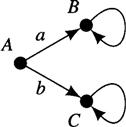
10.6 Consider the state-transition diagram shown here. There are two actions possible from the starting state, A. One, action a, leads to state B and yields an immediate reward of 0. The other, action b, leads to state C and produces an immediate reward of 1000. Once in state B, there is only one action possible. It produces a reward of +1 and leads back to B. Once in state C, there is also only one action possible. It produces a reward of –1 and leads back to C. What temporal discount factor would be required in order to prefer action a to action b?
1 An early AI paper on planning and execution involved a simulated robot and task much like that of Figure 10.4 [Nilsson & Raphael 1967].
2 We might ask why not search to a given cost horizon rather than to a given depth horizon. Since the time required to search usually depends on depth and not cost, we use depth.
3 I discuss this special case simply to introduce some ideas that I later generalize; as I have already said, most problems of practical interest have search spaces too large to list all the nodes.
4 Sutton credits [Samuel 1959] as the originator of the idea.