
9
Heuristic Search
9.1 Using Evaluation Functions
The search processes that I describe in this chapter are something like breadth-first search, except that search does not proceed uniformly outward from the start node; instead, it proceeds preferentially through nodes that heuristic, problem-specific information indicates might be on the best path to a goal. We call such processes best-first or heuristic search. Here is the basic idea.
1. We assume that we have a heuristic (evaluation) function, ![]() , to help decide which node is the best one to expand next. (The reason for the “hat” over the f will become apparent later. We pronounce
, to help decide which node is the best one to expand next. (The reason for the “hat” over the f will become apparent later. We pronounce ![]() “f-hat.”) We adopt the convention that small values of
“f-hat.”) We adopt the convention that small values of ![]() indicate the best nodes. This function is based on information specific to the problem domain. It is a real-valued function of state descriptions.
indicate the best nodes. This function is based on information specific to the problem domain. It is a real-valued function of state descriptions.
2. Expand next that node, n, having the smallest value of ![]() . Resolve ties arbitrarily. (I assume in this chapter that node expansion produces all of the successors of a node.)
. Resolve ties arbitrarily. (I assume in this chapter that node expansion produces all of the successors of a node.)
3. Terminate when the node to be expanded next is a goal node.
People are often able to specify good evaluation functions for best-first search. In the Eight-puzzle, for example, we might try using the number of tiles out of place as a measure of the goodness of a state description:
![]()
Using this heuristic function in the search procedure just described produces the graph shown in Figure 9.1. The numeral next to each node is the value of ![]() for that node.
for that node.
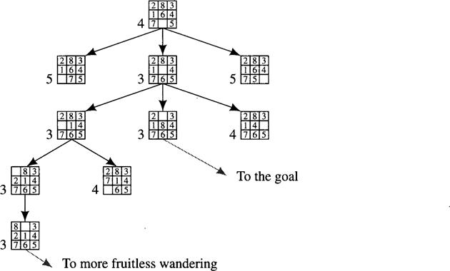
Figure 9.1 A Possible Result of a Heuristic Search Procedure
This example shows that we need to bias the search in favor of going back to explore early paths (in order to prevent being led “down a garden path” by an overly optimistic heuristic). So, we add a “depth factor” to ![]() , where
, where ![]() is an estimate of the “depth” of n in the graph (that is, the length of the shortest path from the start to n), and
is an estimate of the “depth” of n in the graph (that is, the length of the shortest path from the start to n), and ![]() is a heuristic evaluation of node n. If, as before, we let
is a heuristic evaluation of node n. If, as before, we let ![]() = number of tiles out of place (compared with the goal) and take
= number of tiles out of place (compared with the goal) and take ![]() = the depth of node n in the search graph, we get the graph shown in Figure 9.2. In this figure, I have written the values of
= the depth of node n in the search graph, we get the graph shown in Figure 9.2. In this figure, I have written the values of ![]() next to each node. We see that search proceeds rather directly toward the goal in this case (with the exception of the circled node).
next to each node. We see that search proceeds rather directly toward the goal in this case (with the exception of the circled node).

Figure 9.2 Heuristic Search Using ![]()
These examples raise two important questions. First, how do we settle on evaluation functions for guiding best-first search? Second, what are some properties of best-first search? Does it always result in finding good paths to a goal node? Some guidance about evaluation-function selection will be offered toward the end of the chapter, and some methods for automatically learning evaluation functions will be explained in Chapter 10. But most of the chapter will be devoted to a presentation of the formal aspects of best-first search. I begin by developing a general graph search algorithm that includes versions of best-first search as special cases. (For more details about heuristic search than a single chapter or two can provide, refer to the articles cited and to the excellent book by Pearl [Pearl 1984].)
9.2 A General Graph-Searching Algorithm
To be more precise about the heuristic procedures to be explained in this chapter, I need to present a general graph-searching algorithm that permits any kind of ordering the user might prefer—heuristic or uninformed. I call this algorithm GRAPHSEARCH. Here is (a first version of) its definition.
GRAPHSEARCH
1. Create a search tree, Tr, consisting solely of the start node, n0. Put n0 on an ordered list called OPEN.
2. Create a list called CLOSED that is initially empty.
3. If OPEN is empty, exit with failure.
4. Select the first node on OPEN, remove it from OPEN, and put it on CLOSED. Call this node n.
5. If n is a goal node, exit successfully with the solution obtained by tracing a path backward along the arcs in Tr from n to n0. (Arcs are created in step 6.)
6. Expand node n, generating a set, M, of successors. Install M as successors of n in Tr by creating arcs from n to each member of M. Put these members of M on OPEN.
7. Reorder the list OPEN, either according to some arbitrary scheme or according to heuristic merit.
This algorithm can be used to perform best-first search, breadth-first search, or depth-first search. In breadth-first search, new nodes are simply put at the end of OPEN (first in, first out, or FIFO), and the nodes are not reordered. In depth-first-style search, new nodes are put at the beginning of OPEN (last in, first out, or LIFO). In best-first (also called heuristic) search, OPEN is reordered according to the heuristic merit of the nodes.
9.2.1 Algorithm A*
I will particularize GRAPHSEARCH to a best-first search algorithm that reorders (in step 7) the nodes on OPEN according to increasing values of a function ![]() , as in the Eight-puzzle illustration. I will call this version of GRAPHSEARCH, algorithm A*. As we shall see, it will be possible to define
, as in the Eight-puzzle illustration. I will call this version of GRAPHSEARCH, algorithm A*. As we shall see, it will be possible to define ![]() functions that will make A* perform either breadth-first or uniform-cost search. In order to specify the family of
functions that will make A* perform either breadth-first or uniform-cost search. In order to specify the family of ![]() functions to be used, I must first introduce some additional notation.
functions to be used, I must first introduce some additional notation.
Let h(n) = the actual cost of the minimal cost path between node n and a goal node (over all possible goal nodes and over all possible paths from n to them).
Let g(n) = the cost of a minimal cost path from the start node, n0, to node n.
Then f(n) = g(n) + h(n) is the cost of a minimal cost path from no to a goal node over all paths that are constrained to go through node n. Note that f(n0) = h (n0) is then the cost of an (unconstrained) minimal cost path from no to a goal node.
For each node, n, let ![]() (the heuristic factor) be some estimate of h(n), and let
(the heuristic factor) be some estimate of h(n), and let ![]() (the depth factor) be the cost of the lowest-cost path found by A* so far to node n. In algorithm A* we use
(the depth factor) be the cost of the lowest-cost path found by A* so far to node n. In algorithm A* we use ![]() . Note that algorithm A* with
. Note that algorithm A* with ![]() identically 0 gives uniform-cost search. These definitions are illustrated in Figure 9.3.
identically 0 gives uniform-cost search. These definitions are illustrated in Figure 9.3.
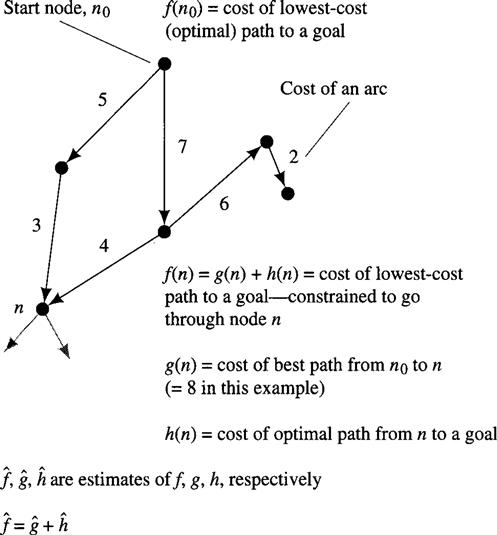
Figure 9.3 Heuristic Search Notation
The search process for the Eight-puzzle illustrated in Figure 9.2 is an example of an application of A*. There, I assumed unit arc costs, so g(n) is simply the depth of node n in the graph. There is a slight complication, though, which I have overlooked in the definition of algorithm A*. What happens if the implicit graph being searched is not a tree? That is, suppose there is more than one sequence of actions that can lead to the same world state from the starting state. For example, the implicit graph of the Eight-puzzle is obviously not a tree because the actions are reversible—each of the successors of any node, n, has n as one of its successors. I ignored these loops in creating the Eight-puzzle search tree. They were easy to ignore in that case; I simply did not include the parent of a node among its successors. Instead of step 6 as written in GRAPHSEARCH, I actually used
6. Expand node n, generating a set, M, of successors that are not already parents of n in Tr. Install M as successors of n in Tr by creating arcs from n to each member of M.
To take care of longer loops, we replace step 6 by
6. Expand node n, generating a set, M, of successors that are not already ancestors of n in Tr. Install M as successors of n in Tr by creating arcs from n to each member of M.
Of course, to check for these longer loops, we need to see if the data structure labeling each successor of node n is equal to the data structure labeling any of node n’s ancestors. For complex data structures, this step can add to the complexity of the algorithm.
The modified step 6 prevents the algorithm from going around in circles in its search for a path to the goal. But there is still the possibility of visiting the same world state via different paths. One way to deal with this problem is simply to ignore it. That is, the algorithm doesn’t check to see if a node in M is already on OPEN or CLOSED. The algorithm is then oblivious to the possibility that it might reach the same node via different paths. This “same node” might then be repeated in Tr as many times as the algorithm discovers different paths to it. If two nodes in Tr are labeled by the same data structure, they will have identical subtrees hanging below them. That is, the algorithm will duplicate search effort that it need not have repeated. We will see later that under very reasonable conditions on ![]() , when A* first expands a node n in Tr, it has already discovered a path to node n having the smallest value of
, when A* first expands a node n in Tr, it has already discovered a path to node n having the smallest value of ![]() .
.
To prevent duplicated search effort when these yet-to-be-mentioned conditions on ![]() do not prevail requires some modification to algorithm A*. Because search might reach the same node along different paths, algorithm A* generates a search graph, which we call G. G is the structure of nodes and arcs generated by A* as it expands the start node, its successors, and so on. A* also maintains a search tree, Tr. Tr, a subgraph of G, is the tree of best (minimal cost) paths produced so far to all of the nodes in the search graph. I show examples for a graph having unit arc costs in Figure 9.4. An early stage of search is shown in Figure 9.4a. The search-tree part of the search graph is indicated by the dark arcs; gray arcs are in the search graph but not the search tree. The dark arcs indicate the least costly paths found so far to the nodes in the search graph. Note that node 4 in Figure 9.4a has been reached by two paths; both paths are in the search graph, but only one is in the search tree. We keep the search graph because subsequent search may find shorter paths that use some of the arcs in the earlier search graph that were not in the earlier search tree. For example, in Figure 9.4b, expanding node 1 finds shorter paths to node 2 and its descendants (including node 4), so the search tree is changed accordingly.
do not prevail requires some modification to algorithm A*. Because search might reach the same node along different paths, algorithm A* generates a search graph, which we call G. G is the structure of nodes and arcs generated by A* as it expands the start node, its successors, and so on. A* also maintains a search tree, Tr. Tr, a subgraph of G, is the tree of best (minimal cost) paths produced so far to all of the nodes in the search graph. I show examples for a graph having unit arc costs in Figure 9.4. An early stage of search is shown in Figure 9.4a. The search-tree part of the search graph is indicated by the dark arcs; gray arcs are in the search graph but not the search tree. The dark arcs indicate the least costly paths found so far to the nodes in the search graph. Note that node 4 in Figure 9.4a has been reached by two paths; both paths are in the search graph, but only one is in the search tree. We keep the search graph because subsequent search may find shorter paths that use some of the arcs in the earlier search graph that were not in the earlier search tree. For example, in Figure 9.4b, expanding node 1 finds shorter paths to node 2 and its descendants (including node 4), so the search tree is changed accordingly.

Figure 9.4 Search Graphs and Trees Produced by a Search Procedure
For completeness, I state the version of A* that maintains the search graph. We note, however, that this version is seldom needed because we can usually impose conditions on ![]() that guarantee that when algorithm A* expands a node, it has already found the least costly path to that node.
that guarantee that when algorithm A* expands a node, it has already found the least costly path to that node.
Algorithm A*
1. Create a search graph, G, consisting solely of the start node, no. Put no on a list called OPEN.
2. Create a list called CLOSED that is initially empty.
3. If OPEN is empty, exit with failure.
4. Select the first node on OPEN, remove it from OPEN, and put it on CLOSED. Call this node n.
5. If n is a goal node, exit successfully with the solution obtained by tracing a path along the pointers from n to n0 in G. (The pointers define a search tree and are established in step 7.)
6. Expand node n, generating the set, M, of its successors that are not already ancestors of n in G. Install these members of M as successors of n in G.
7. Establish a pointer to n from each of those members of M that were not already in G (i.e., not already on either OPEN or CLOSED). Add these members of M to OPEN. For each member, m, of M that was already on OPEN or CLOSED, redirect its pointer to n if the best path to m found so far is through n. For each member of M already on CLOSED, redirect the pointers of each of its descendants in G so that they point backward along the best paths found so far to these descendants.
8. Reorder the list OPEN in order of increasing ![]() . values. (Ties among minimal
. values. (Ties among minimal ![]() values are resolved in favor of the deepest node in the search tree.)
values are resolved in favor of the deepest node in the search tree.)
In step 7, we redirect pointers from a node if the search process discovers a path to that node having lower cost than the one indicated by the existing pointers. Redirecting pointers of descendants of nodes already on CLOSED saves subsequent search effort but at the possible expense of an exponential amount of computation. Hence this part of step 7 is often not implemented. Some of these pointers will ultimately be redirected in any case as the search progresses.
9.2.2 Admissibility of A*
There are conditions on graphs and on ![]() that guarantee that algorithm A* applied to these graphs always finds minimal cost paths. The conditions on the graphs are
that guarantee that algorithm A* applied to these graphs always finds minimal cost paths. The conditions on the graphs are
1. Each node in the graph has a finite number of successors (if any).
2. All arcs in the graph have costs greater than some positive amount, ∈.
The condition on ![]() is
is
3. For all nodes n in the search graph, ![]() . That is,
. That is, ![]() never overestimates the actual value, h. (Such an
never overestimates the actual value, h. (Such an ![]() function is sometimes called an optimistic estimator.)
function is sometimes called an optimistic estimator.)
Often, it is not difficult to find an ![]() function that satisfies this lower bound condition. For example, in route-finding problems over a graph whose nodes consist of cities, the straight-line distance from a city, n, to a goal city is a lower bound on the distance of an optimal route from n to the goal node. In the Eight-puzzle, the number of tiles out of place is a lower bound on the number of steps remaining to the goal.
function that satisfies this lower bound condition. For example, in route-finding problems over a graph whose nodes consist of cities, the straight-line distance from a city, n, to a goal city is a lower bound on the distance of an optimal route from n to the goal node. In the Eight-puzzle, the number of tiles out of place is a lower bound on the number of steps remaining to the goal.
With these three conditions, algorithm A* is guaranteed to find an optimal path to a goal, if any path to a goal exists. I can state this result as a theorem. (I give a new version of a proof of this theorem next; for the original proof, see [Hart, Nilsson, & Raphael 1968].)
Theorem 9.1
Under the conditions on graphs and on ![]() stated earlier, and providing there is a path with finite cost from the start node, n0, to a goal node, algorithm A* is guaranteed to terminate with a minimal-cost path to a goal.
stated earlier, and providing there is a path with finite cost from the start node, n0, to a goal node, algorithm A* is guaranteed to terminate with a minimal-cost path to a goal.
Proof: The main component of the proof is the following important lemma. It is important to understand this lemma thoroughly in order to gain intuition about why A* is guaranteed to find optimal paths.
Lemma 9.1
At every step before termination of A*, there is always a node, say, n*, on OPEN with the following properties:
Proof of Lemma: To prove that the conclusions of the lemma hold at every step of A*, it suffices to prove that (1) they hold at the beginning of the algorithm and (2) if they hold before a node expansion, they will continue to hold after a node expansion. We call this kind of proof, proof by mathematical induction. Here is how it goes.
Base case: At the beginning of search (when just node n0 has been selected for expansion), node n0 is on OPEN, it is on an optimal path to the goal, and A* has found this path. Also ![]() because
because ![]() ≤ f(n0). Thus, node no can be the node n* of the lemma at this stage.
≤ f(n0). Thus, node no can be the node n* of the lemma at this stage.
Induction step: We assume the conclusions of the lemma at the time m nodes have been expanded (m ≥ 0) and (using this assumption) prove them true at the time m + 1 nodes have been expanded. It may be helpful to refer to Figure 9.5 as we prove the induction step.
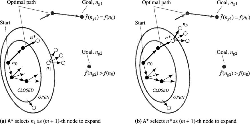
Figure 9.5 The Situation When the (m + l)–th Node Is Selected for Expansion
We let n* be the hypothesized node on OPEN, which is on an optimal path found by A* after it has expanded m nodes. Now, if n* is not selected for expansion on the (m + l)-th step (Figure 9.5a), n* has the same properties as before, thus proving the induction step for that case. If n* is selected for expansion (Figure 9.5b), all of its new successors will be put on OPEN, and at least one of them, say, np, will be on an optimal path to a goal (since an optimal path is hypothesized to go through n* and it must continue through one of its successors). And A* has found an optimal path to np because, if there were a better path to np, that better path would also be a better path to a goal (contradicting our hypothesis that there is no better path to the goal than the one A* has found through n*). So, in this case, we let np be the new n* for the (m + l)-th step, and we have proved the induction step except for the property that ![]() .
.
We prove that property now for all steps m before termination. For any node, n*, on an optimal path and to which A* has found an optimal path, we have
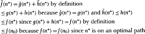
which completes a proof of the lemma.
Continuing now with the proof of the theorem, we prove first that A* must terminate if there is an accessible goal, and then that it terminates by finding an optimal path to a goal.
• A* must terminate: Suppose it does not terminate. In that case, A* continues to expand nodes on OPEN forever and would eventually expand nodes deeper in the search tree than any preset finite depth bound—since we have assumed that the graph being searched has finite branching factor. Since the cost of each arc is larger than ε > 0, the ![]() (and thus the
(and thus the ![]() .) values of all nodes on OPEN will eventually exceed f(n0). But that would contradict the lemma.
.) values of all nodes on OPEN will eventually exceed f(n0). But that would contradict the lemma.
• A* terminates in an optimal path: A* can terminate only in step 3 (if OPEN is empty) or in step 5 (in a goal node). A step 3 termination can occur only for finite graphs containing no goal node, and the theorem claims to find an optimal path to a goal only if there is a goal node. Therefore, A* terminates by finding a goal node. Suppose it terminates by finding a nonoptimal goal, say, ng2 with f(ng2) > f(n0) when there is an optimal goal, say, ng1 ν ng2 with f(ng1) =f(n0) (see Figure 9.5 again). At termination in ng2, ![]() . But just before A* selected ng2 for expansion, by the lemma there was a node n* on OPEN and on an optimal path with
. But just before A* selected ng2 for expansion, by the lemma there was a node n* on OPEN and on an optimal path with ![]() . Thus, A* could not have selected ng2 for expansion because A* always selects that node having the smallest value of
. Thus, A* could not have selected ng2 for expansion because A* always selects that node having the smallest value of ![]() and
and ![]() .
.
This completes the proof of the theorem. We say that any algorithm that is guaranteed to find an optimal path to the goal is admissible. Thus, with the three conditions of the theorem, A* is admissible. By extension, we say that any ![]() function that does not overestimate
function that does not overestimate ![]() is admissible. From now on, when I talk about applying A*, I assume that the three conditions of the theorem are satisfied.
is admissible. From now on, when I talk about applying A*, I assume that the three conditions of the theorem are satisfied.
If two versions of A*, namely, A1* and A2*, differ only in that ![]() for all nongoal nodes, we will say that A2* is more informed than A1*. I state the following result without proof (see [Hart, Nilsson, & Raphael 1968, Hart, Nilsson, & Raphael 1972, Nilsson 1980]).
for all nongoal nodes, we will say that A2* is more informed than A1*. I state the following result without proof (see [Hart, Nilsson, & Raphael 1968, Hart, Nilsson, & Raphael 1972, Nilsson 1980]).
Theorem 9.2
If ![]() is more informed than
is more informed than![]() then at the termination of their searches on any graph having a path from n0 to a goal node, every node expanded by
then at the termination of their searches on any graph having a path from n0 to a goal node, every node expanded by ![]() is also expanded by
is also expanded by ![]() .
.
It follows that ![]() expands at least as many nodes as does
expands at least as many nodes as does ![]() , and thus the more informed algorithm, is typically more efficient. Thus,
, and thus the more informed algorithm, is typically more efficient. Thus, ![]() we seek an
we seek an ![]() function whose values are as close as possible to those of the actual
function whose values are as close as possible to those of the actual ![]() function (for search efficiency), while still not exceeding them (for admissibility). Of course, in measuring total search efficiency, we should also take into account the cost of computing
function (for search efficiency), while still not exceeding them (for admissibility). Of course, in measuring total search efficiency, we should also take into account the cost of computing ![]() . The most informed algorithm would have
. The most informed algorithm would have ![]() , but, typically, such an
, but, typically, such an ![]() function could be obtained only at high cost by completing the very search we are attempting!
function could be obtained only at high cost by completing the very search we are attempting!
Figure 9.6 summarizes relationships among some of the search algorithms we have discussed. When ![]() for all nodes, we have a uniform-cost algorithm. (The search spreads out along contours of equal cost.) When
for all nodes, we have a uniform-cost algorithm. (The search spreads out along contours of equal cost.) When ![]() , we have breadth-first search, which spreads out along contours of equal depth. Both the uniform-cost and breadth-first algorithms are special cases of A* (with
, we have breadth-first search, which spreads out along contours of equal depth. Both the uniform-cost and breadth-first algorithms are special cases of A* (with ![]() ), so, of course, they are both admissible.
), so, of course, they are both admissible.
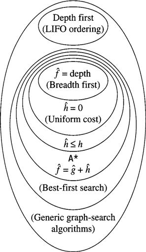
Figure 9.6 Relationships Among Search Algorithms
9.2.3 The Consistency (or Monotone) Condition
Consider a pair of nodes such that nj is a successor of ni. We say that ![]() obeys the consistency condition if, for all such pairs in the search graph,
obeys the consistency condition if, for all such pairs in the search graph,
![]()
where c(ni, nj) is the cost of the arc from ni to nj We could also write
![]()
and
![]()
This condition states that along any path in the search graph, our estimate of the optimal (remaining) cost to the goal cannot decrease by more than the arc cost along that path. That is, the heuristic function is locally consistent taking into account the known cost of an arc.1 The consistency condition can also be thought of as a type of triangle inequality as shown in Figure 9.7.
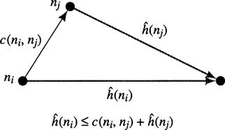
Figure 9.7 The Consistency Condition
The consistency condition also implies that the ![]() . values of the nodes in the search tree are monotonically nondecreasing as we move away from the start node. Let ni and nj be two nodes in the search tree generated by A* with nj a successor of ni. Then, if the consistency condition is satisfied,
. values of the nodes in the search tree are monotonically nondecreasing as we move away from the start node. Let ni and nj be two nodes in the search tree generated by A* with nj a successor of ni. Then, if the consistency condition is satisfied, ![]() . To prove this fact, we start with the consistency condition:
. To prove this fact, we start with the consistency condition:
![]()
We then add ![]() to both sides:
to both sides:
![]()
But ![]() . (We might worry that
. (We might worry that ![]() might be lower than this value because we might have arrived at nj along some path less costly than that through ni. But then nj would not be a successor of ni in the search tree.) Thus,
might be lower than this value because we might have arrived at nj along some path less costly than that through ni. But then nj would not be a successor of ni in the search tree.) Thus,
![]()
For this reason, the consistency condition (on ![]() ) is often called the monotone condition (on
) is often called the monotone condition (on ![]() .).
.).
We have an important theorem involving the consistency condition ([Hart, Nilsson, & Raphael 1968]).
Theorem 9.3
If the consistency condition on ![]() is satisfied, then when A* expands a node n, it has already found an optimal path to n.
is satisfied, then when A* expands a node n, it has already found an optimal path to n.
Proof: Suppose A* is about to expand an open node, n, in a search for an optimal path from a start node, n0, to a goal node in an implicit graph, G. Let ξ = (n0, n1, …, nl, nl+1, …, n = nk) be a sequence of nodes in G constituting an optimal path from n0 to n. Let nl be the last node on ξ expanded by A*. (See Figure 9.8.) Because nl is the last closed node on ξ, we know that nl+1 is on OPEN and thus a candidate for expansion.

Figure 9.8 Graph Used in Proof of Theorem 9.3
For any node, ni, and its successor, ni+1, in ξ (an optimal path to n), we have
![]()
![]() when the consistency condition is satisfied
when the consistency condition is satisfied
Transitivity of the ≥ relation gives us
![]()

But since A* is about to expand node n instead of node nl+1, it must be the case that
![]()
But we have already established that
![]()
Therefore,
![]()
But since our method for computing the ![]() ’s implies that
’s implies that ![]() , it must be the case that
, it must be the case that
![]()
which completes the proof, showing either that nl+1 = n or that we must already have found some other optimal path to node n.
The consistency condition is important because when it is satisfied, A* never has to redirect pointers (in step 7). Searching a graph is then no different from searching a tree.
With the consistency condition satisfied, we can give a simple, intuitive argument for the admissibility of A*. It goes like this:
1. Monotonicity of ![]() . implies that search expands outward along contours of increasing
. implies that search expands outward along contours of increasing ![]() . values.
. values.
2. Thus, the first goal node selected will be a goal node having a minimal ![]() value.
value.
3. For any goal node, ![]() . (Here, we use the fact that if the
. (Here, we use the fact that if the ![]() function is consistent it will also never be greater than the true h function [Pearl 1984, p. 83].)
function is consistent it will also never be greater than the true h function [Pearl 1984, p. 83].)
4. Thus, the first goal node selected will be one having minimal ĝ value.
5. As a consequence of Theorem 9.3, whenever (in particular) a goal node, ng, is selected for expansion, we have found an optimal path to that goal node. That is, ![]() .
.
6. Thus, the first goal node selected will be one for which the algorithm has found an optimal path.
Many heuristic functions satisfy the consistency condition. For example, the “tiles-out-of-place” function in the Eight-puzzle does. When a heuristic function does not satisfy the consistency condition, but is otherwise admissible, then (using an idea proposed by Mérõ [Mérõ 1984]) we can adjust it (during search) to one that does satisfy the consistency condition. Suppose, at every step of A* we check the ![]() values of the successors of the node, say, n, just expanded. Any of these whose
values of the successors of the node, say, n, just expanded. Any of these whose ![]() values are smaller than
values are smaller than ![]() (n) minus the arc cost from n to that successor will have their
(n) minus the arc cost from n to that successor will have their ![]() values adjusted (during search) so that they are exactly equal to
values adjusted (during search) so that they are exactly equal to ![]() (n) minus that arc cost. (But it is possible that a node on CLOSED that has its
(n) minus that arc cost. (But it is possible that a node on CLOSED that has its ![]() value adjusted in this way may have to be moved back to OPEN.) I leave it to you to verify that this adjustment leaves the algorithm admissible.
value adjusted in this way may have to be moved back to OPEN.) I leave it to you to verify that this adjustment leaves the algorithm admissible.
9.2.4 Iterative-Deepening A*
In Chapter 8,1 stated that the memory requirements of breadth-first search grew exponentially with the depth of the goal in the search space. Heuristic search has the same disadvantage although good heuristics do reduce the branching factor. Iterative-deepening search, introduced in Chapter 8, allows us to find minimal-cost paths with memory that grows only linearly with the depth of the goal. A method called iterative-deepening A* (IDA*), proposed by [Korf 1985], can achieve a similar benefit for heuristic search. Further efficiencies can be gained by using a parallel implementation of IDA* (see [Powley, Ferguson, & Korf 1993]).
The method works in a manner similar to ordinary iterative deepening. We execute a series of depth-first searches. In the first search, we establish a “cost cut-off” equal to ![]() , where n0 is the start node. For all we know, the cost of an optimal path to a goal may equal this cut-off value. (It will if
, where n0 is the start node. For all we know, the cost of an optimal path to a goal may equal this cut-off value. (It will if ![]() ; it cannot be less because
; it cannot be less because ![]() .) We expand nodes in depth-first fashion—backtracking whenever the f value of a successor of an expanded node exceeds the cut-off value. If this depth-first search terminates at a goal node, it obviously has found a minimal-cost path to a goal. If it does not, then the cost of an optimal path must be greater than the cut-off value. So, we increase the cut-off value and start another depth-first search. What is the next possibility for the cost of an optimal path? It might be as low as the lowest of the
.) We expand nodes in depth-first fashion—backtracking whenever the f value of a successor of an expanded node exceeds the cut-off value. If this depth-first search terminates at a goal node, it obviously has found a minimal-cost path to a goal. If it does not, then the cost of an optimal path must be greater than the cut-off value. So, we increase the cut-off value and start another depth-first search. What is the next possibility for the cost of an optimal path? It might be as low as the lowest of the ![]() values of the nodes visited (but not expanded) in the previous depth-first search. The node having this lowest
values of the nodes visited (but not expanded) in the previous depth-first search. The node having this lowest ![]() value might be on an optimal path (now that we know that no optimal path exists having cost equal to the previous cut-off value). This lowest
value might be on an optimal path (now that we know that no optimal path exists having cost equal to the previous cut-off value). This lowest ![]() value is used as the new cut-off value in the next depth-first search. And so on. Intuitively, it is easy to see that IDA* is guaranteed to find a minimal-cost path to a goal. ([Korf 1985] presents a proof of this result, as does [Korf 1993]. The latter work also discusses limitations of iterative deepening in the case in which the monotone condition is not satisfied and presents an alternative algorithm called recursive best-first search.)
value is used as the new cut-off value in the next depth-first search. And so on. Intuitively, it is easy to see that IDA* is guaranteed to find a minimal-cost path to a goal. ([Korf 1985] presents a proof of this result, as does [Korf 1993]. The latter work also discusses limitations of iterative deepening in the case in which the monotone condition is not satisfied and presents an alternative algorithm called recursive best-first search.)
IDA* does have to repeat node expansions, but (as with ordinary iterative deepening) there are potential tradeoffs involving the reduced memory requirements and the implementational efficiencies of depth-first search (as compared with breadth-first search). But note what happens in the case in which all of the ![]() values are different for each node in the search space—the number of iterations can equal the number of nodes having
values are different for each node in the search space—the number of iterations can equal the number of nodes having ![]() values less than the cost of an optimal path! (There are ways to ameliorate this problem at the price of giving up admissibility. I leave it to you to invent how this might be done.)
values less than the cost of an optimal path! (There are ways to ameliorate this problem at the price of giving up admissibility. I leave it to you to invent how this might be done.)
9.2.5 Recursive Best-First Search
A search method proposed by Korf called recursive best-first search, RBFS ([Korf 1993]), uses slightly more memory than does IDA* but generates fewer nodes than does IDA*. When a node, say, n, is expanded, RBFS computes the ![]() values of the successors of n and recomputes the
values of the successors of n and recomputes the ![]() values of n and all of n’s ancestors in the search tree. This recomputation process is called backing up the
values of n and all of n’s ancestors in the search tree. This recomputation process is called backing up the ![]() values. Backing up is done as follows: The backed-up value of a successor of the node just expanded is simply the
values. Backing up is done as follows: The backed-up value of a successor of the node just expanded is simply the ![]() value of that successor. The backed-up value,
value of that successor. The backed-up value, ![]() (m), of node m in the search tree with successors mi is
(m), of node m in the search tree with successors mi is
![]()
where ![]() (mi) is the backed-up value of node mi.
(mi) is the backed-up value of node mi.
If one of those successors of node n (which was just expanded) has the smallest value of ![]() over all OPEN nodes, it is expanded in turn, and so on. But suppose some other OPEN node, say, n‘—not a successor of n—has the lowest value of
over all OPEN nodes, it is expanded in turn, and so on. But suppose some other OPEN node, say, n‘—not a successor of n—has the lowest value of ![]() . In that case, the algorithm backtracks to the lowest common ancestor, say, node k, of nodes n‘ and n. Let node kn be the successor of node k on the path to n. RBFS removes the subtree rooted at kn, kn becomes an OPEN node with
. In that case, the algorithm backtracks to the lowest common ancestor, say, node k, of nodes n‘ and n. Let node kn be the successor of node k on the path to n. RBFS removes the subtree rooted at kn, kn becomes an OPEN node with ![]() value equal to its backed-up value, and search continues below that OPEN node, namely, n‘, with the lowest value of
value equal to its backed-up value, and search continues below that OPEN node, namely, n‘, with the lowest value of ![]() .
.
I illustrate the main idea of this algorithm in Figure 9.9. At all times, the search tree consists of a single path of nodes plus the siblings of all nodes on the path. Thus, the storage requirements are still linear in the length of the best path explored so far. The tip nodes are all on OPEN, and all nodes in the search tree have associated backed-up ![]() values.
values.
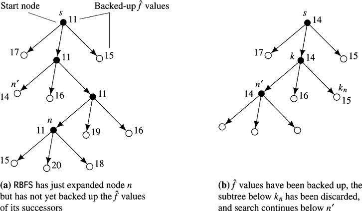
Figure 9.9 Recursive Best-First Search
For a review of and citations to other space-efficient search algorithms, see [Korf 1996].
9.3 Heuristic Functions and Search Efficiency
The selection of the heuristic function is crucial in determining the efficiency of A*. Using ![]() ≡ 0 assures admissibility but results in a uniform-cost search and is thus usually inefficient. Setting
≡ 0 assures admissibility but results in a uniform-cost search and is thus usually inefficient. Setting ![]() equal to the highest possible lower bound on
equal to the highest possible lower bound on ![]() expands the fewest nodes consistent with maintaining admissibility. In the Eight-puzzle, for example, the function
expands the fewest nodes consistent with maintaining admissibility. In the Eight-puzzle, for example, the function ![]() (where W (n) is the number of tiles in the wrong place) is a lower bound on
(where W (n) is the number of tiles in the wrong place) is a lower bound on ![]() (n), but it does not provide a very good estimate of the difficulty (in terms of number of steps to the goal) of a tile configuration. A better estimate is the function
(n), but it does not provide a very good estimate of the difficulty (in terms of number of steps to the goal) of a tile configuration. A better estimate is the function ![]() , where P(n) is the sum of the (Manhattan) distances that each tile is from “home” (ignoring intervening pieces).
, where P(n) is the sum of the (Manhattan) distances that each tile is from “home” (ignoring intervening pieces).
Early in the history of AI, [Newell, Shaw, & Simon 1959, Newell 1964] suggested using a simplified model to form a “plan” to guide search. Similar ideas, applied to the problem of finding a good heuristic function, are described by [Gaschnig 1979] and by [Pearl 1984, Ch. 4]. For example, we can relax the conditions of the Eight-puzzle by allowing less restrictive tile movements. If we allow a tile to move directly (in one step) to its goal square, then the number of steps to the goal is just the sum of the number of tiles in the wrong place, W (n). A less relaxed (and therefore better) model allows tiles to move to an adjacent square even though there may already be a tile there. The number of steps to a goal for this model is the sum of the distances that each tile is from its goal square, P(n). These models show how an agent might automatically calculate the ![]() functions we intuitively guessed. Pearl points out that we might have calculated an
functions we intuitively guessed. Pearl points out that we might have calculated an ![]() function that is slightly better than W (n) by using a model in which any tile can be swapped with the blank position in one move. Another less relaxed model would be one in which tiles can move only to the position of the blank cell along a path of adjacent cells—counting each position along the path as a move.
function that is slightly better than W (n) by using a model in which any tile can be swapped with the blank position in one move. Another less relaxed model would be one in which tiles can move only to the position of the blank cell along a path of adjacent cells—counting each position along the path as a move.
The use of Euclidean (straight-line) distances as ![]() functions in road-map navigation problems can also be explained by relaxed models. Instead of having to travel over existing roads, a traveler in a relaxed model can “tele-transport” directly to any city using a straight-line distance. Since solutions in relaxed models are never more costly than solutions in the original problem, the
functions in road-map navigation problems can also be explained by relaxed models. Instead of having to travel over existing roads, a traveler in a relaxed model can “tele-transport” directly to any city using a straight-line distance. Since solutions in relaxed models are never more costly than solutions in the original problem, the ![]() functions so selected are always admissible! It turns out that they are also consistent, so algorithms using them do not have to revisit previously expanded nodes.
functions so selected are always admissible! It turns out that they are also consistent, so algorithms using them do not have to revisit previously expanded nodes.
In selecting an ![]() function, we must take into consideration the amount of effort involved in calculating it. The less relaxed the model, the better will be the heuristic function—although typically the more difficult it will be to calculate. The absolute minimum number of node expansions is achieved if one uses a heuristic function identically equal to
function, we must take into consideration the amount of effort involved in calculating it. The less relaxed the model, the better will be the heuristic function—although typically the more difficult it will be to calculate. The absolute minimum number of node expansions is achieved if one uses a heuristic function identically equal to ![]() , but the calculation of such an
, but the calculation of such an ![]() would require solving the original problem. There is usually a tradeoff between the benefits gained by an accurate
would require solving the original problem. There is usually a tradeoff between the benefits gained by an accurate ![]() function and the cost of computing it.
function and the cost of computing it.
Often, search efficiency can be gained at the expense of admissibility by using some function for ![]() that is not a lower bound on
that is not a lower bound on ![]() . That is, a possibly nonoptimal path might be easier to find than would be a guaranteed optimal one. And an
. That is, a possibly nonoptimal path might be easier to find than would be a guaranteed optimal one. And an ![]() function that is not a lower bound on
function that is not a lower bound on ![]() might be easier to compute than one that is a lower bound. In these cases, efficiency might be doubly improved—because the total number of nodes expanded can be reduced (albeit at the expense of admissibility) and because the computational effort is reduced.
might be easier to compute than one that is a lower bound. In these cases, efficiency might be doubly improved—because the total number of nodes expanded can be reduced (albeit at the expense of admissibility) and because the computational effort is reduced.
Another possibility is to modify the relative weights of ![]() and
and ![]() in the evaluation function. That is, we use
in the evaluation function. That is, we use ![]() , where w is a positive number. Very large values of w overemphasize the heuristic component, whereas very small values of w give the search a predominantly breadth-first character. Experimental evidence suggests that search efficiency is often enhanced by allowing the value of w to vary inversely with the depth of a node in the search tree. At shallow depths, the search relies mainly on the heuristic component, whereas at greater depths, the search becomes increasingly breadth first, to ensure that some path to a goal will eventually be found.
, where w is a positive number. Very large values of w overemphasize the heuristic component, whereas very small values of w give the search a predominantly breadth-first character. Experimental evidence suggests that search efficiency is often enhanced by allowing the value of w to vary inversely with the depth of a node in the search tree. At shallow depths, the search relies mainly on the heuristic component, whereas at greater depths, the search becomes increasingly breadth first, to ensure that some path to a goal will eventually be found.
We might think that search efficiency could be improved by conducting simultaneous searches from both the start node and a goal node. Such improvements can, typically be achieved only for breadth-first searches. When a breadth-first search is used in both directions, we can be assured that the search frontiers meet somewhere between start and goal (see Figure 9.10a), and termination conditions have been established so that the breadth-first bidirectional search is guaranteed to find an optimal path [Pohl 1971]. But if heuristic search is initiated at both start and goal nodes, the two search frontiers might not meet to produce an optimal path if the heuristic tends to focus the searches in inappropriate directions. (See Figure 9.10b.)

Figure 9.10 Bidirectional Searches
A useful measure of search efficiency is the effective branching factor, B. It describes how sharply a search process is focussed toward the goal. Suppose that search finds a path of length d and generates a total of N nodes. B is then equal to the number of successors of each node in that tree having the following properties:
• Each nonleaf node in the tree has the same number (B) of successors.
Therefore, B is related to path length d and to the total number of nodes generated, N, by the expressions
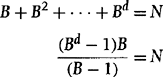
Although B cannot be written explicitly as a function of d and N, a plot of B versus N for various values of d is given in Figure 9.11. A value of B near unity corresponds to a search that is highly focussed toward the goal, with very little branching in other directions. On the other hand, a “bushy” search graph would have a high B value.
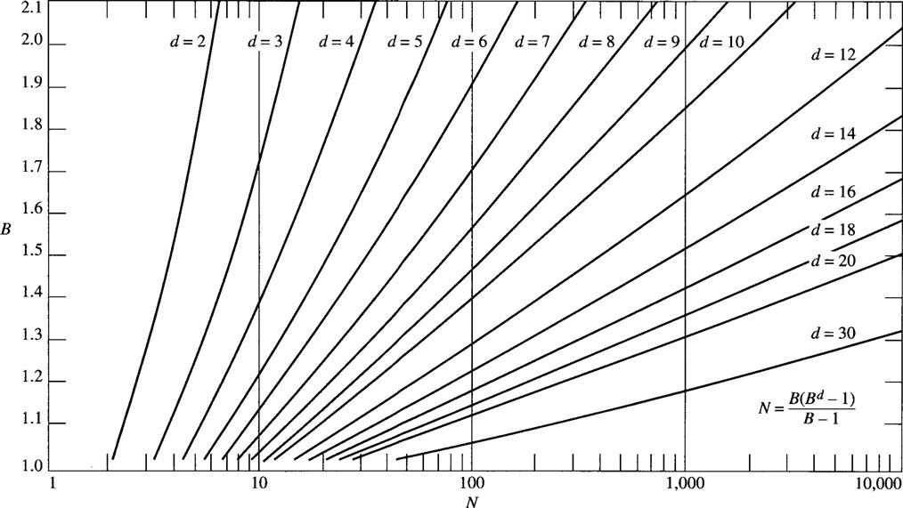
Figure 9.11 B Versus N for Various Values of d
To the extent that the effective branching factor is reasonably independent of path length, it can be used to give an estimate of how many nodes might be generated in searches of various lengths. For example, we can use Figure 9.11 to calculate that the use of the evaluation function ![]() results in a B value equal to 1.2 for the Eight-puzzle problem illustrated in Figure 9.2. Suppose we wanted to estimate how many nodes would be generated using this same evaluation function in solving a more difficult Eight-puzzle problem, say, one requiring 30 steps. From Figure 9.11, we note that the 30-step puzzle would involve the generation of about 2000 nodes, assuming that the effective branching factor remained constant.
results in a B value equal to 1.2 for the Eight-puzzle problem illustrated in Figure 9.2. Suppose we wanted to estimate how many nodes would be generated using this same evaluation function in solving a more difficult Eight-puzzle problem, say, one requiring 30 steps. From Figure 9.11, we note that the 30-step puzzle would involve the generation of about 2000 nodes, assuming that the effective branching factor remained constant.
To summarize, there are three important factors influencing the efficiency of algorithm A*:
The selection of a suitable heuristic function permits us to balance these factors to maximize search efficiency.
All of the search methods discussed so far, including the heuristic ones, have 0(n) time complexity, where n is the number of nodes generated (assuming that the heuristic function can be computed in constant time). In particular, the complexity is 0(Bd) for breadth-first search when the effective branching factor is B, the arc costs are all equal, and goals are of depth d away from the start node. For uniform-cost search (that is, ![]() ≡ 0) and unequal arc costs, the complexity is 0(BC/c), where C is the cost of an optimal solution and c is the cost of the least costly arc [Korf 1992]. For many problems of practical interest, d (or C/c) is sufficiently large to make search (even heuristic search) for optimal solutions computationally infeasible. For example, if we are using search to compute the best next action (out of, say, four choices) when the goal being sought is 15 actions away, the search algorithm may have to expand as many as 415 ≈ 109 nodes. Such lengthy calculations might not be practical in cases in which an agent must make a decision in a fraction of a second. Space complexity for A* is of the same order as time complexity because all nodes expanded have to be stored in a tree structure.
≡ 0) and unequal arc costs, the complexity is 0(BC/c), where C is the cost of an optimal solution and c is the cost of the least costly arc [Korf 1992]. For many problems of practical interest, d (or C/c) is sufficiently large to make search (even heuristic search) for optimal solutions computationally infeasible. For example, if we are using search to compute the best next action (out of, say, four choices) when the goal being sought is 15 actions away, the search algorithm may have to expand as many as 415 ≈ 109 nodes. Such lengthy calculations might not be practical in cases in which an agent must make a decision in a fraction of a second. Space complexity for A* is of the same order as time complexity because all nodes expanded have to be stored in a tree structure.
Since agents will have time and memory bounds on their computational resources, it will be impossible to find optimal solutions for many tasks. Instead, it will be necessary to settle either for nonoptimal but acceptable solutions (called satisficing solutions) or for partial solutions. In the next chapter, I will present a variety of methods that can be used by agents with limited resources.
9.4 Additional Readings and Discussion
Heuristic search involves two kinds of computations. First, there is the object-level computation of actually expanding nodes and producing the path itself. Second, there is the metalevel computation of deciding which node to expand next. The object level is about physical actions in the world; the metalevel is about computational actions in the graph. Object-level/metalevel distinctions come up frequently in AI. They are thoroughly discussed in [Russell & Wefald 1991] and play a particularly important role in the abbreviated search methods to be discussed in the next chapter.
Sliding block puzzles have been used by many AI researchers as a testbed problem for heuristic search methods. An early paper by [Doran & Michie 1966] used the Eight-puzzle and initiated the use of evaluation functions in procedures for finding paths in graphs.
In 1990, Korf stated that while “IDA* can solve the Fifteen-puzzle, any larger puzzle [such as the Twenty-four puzzle] is intractable on current machines” [Korf 1990, p. 191], Yet with a more powerful machine (a Sun Ultra Sparc workstation generating a million nodes per second) and with more powerful (automatically discovered) heuristics, [Korf & Taylor 1996] were able to find optimal solutions to randomly generated, solvable instances of the Twenty-four puzzle in times ranging between two and a quarter hours and a month. [Korf 1997] used IDA* to find optimal solutions to the 3 × 3 × 3 Rubik’s Cube puzzle.
Although puzzles have been useful for improving and testing search techniques, A* and related heuristic search procedures have been successfully applied to many practical problems.
For more on using relaxed models to discover heuristic functions, see [Mostow & Prieditis 1989, Prieditis 1993]. [Pohl 1973] experimented with varying the weight on the heuristic component of ![]() .
.
The classic book on heuristic search is [Pearl 1984]. [Kanal & Kumar 1988] is a collection of papers about search. The first paper in the latter book proposes a unification of search methods developed independently by AI and operations research people.
Exercises
9.1 In the “Four-Queens puzzle,” we try to place four queens on a 4 × 4 chess board so that none can capture any other. (That is, only one queen can be on any row, column, or diagonal of the array.) Suppose we try to solve this puzzle using the following problem space: The start node is labeled by an empty 4 × 4 array; the successor function creates new 4×4 arrays containing one additional legal placement of a queen anywhere in the array; the goal predicate is satisfied if and only if there are four queens in the array (legally positioned).
1. Invent an admissible heuristic function for this problem based on the number of queen placements remaining to achieve the goal. (Note that all goal nodes are precisely four steps from the start node!)
2. Use your heuristic function in an A* search to a goal node. Draw the search tree consisting of all 4 × 4 arrays produced by the search and label each array by its value of g and ![]() . (Note that symmetry considerations mean we have to generate only three successors of the start node.)
. (Note that symmetry considerations mean we have to generate only three successors of the start node.)
9.2 This exercise assumes you have already completed Exercise 7.4 about the Tower-of-Hanoi puzzle. Refer to your solution to that exercise, or, if you have not already done it, do it now before continuing. Propose an admissible ![]() function for this problem that is better than
function for this problem that is better than ![]() ≡ 0.
≡ 0.
9.3 Algorithm A* does not terminate until a goal node is selected for expansion. However, a path to a goal node might be reached long before that node is selected for expansion. Why not terminate as soon as a goal node has been found? Illustrate your answer with an example.
9.4 The monotone condition on the heuristic function requires that ![]() for all node-successor pairs (ni, nj), where c(ni, nj) is the cost on the arc from ni to nj. It has been suggested that when the monotone condition is not satisfied, this fact can be discovered and
for all node-successor pairs (ni, nj), where c(ni, nj) is the cost on the arc from ni to nj. It has been suggested that when the monotone condition is not satisfied, this fact can be discovered and ![]() adjusted during search so that the condition is satisfied. The idea is that whenever a node ni is expanded, with successor node nj, we can increment
adjusted during search so that the condition is satisfied. The idea is that whenever a node ni is expanded, with successor node nj, we can increment ![]() by whatever amount is needed to satisfy the monotone condition. Construct an example to show that even with this scheme, when a node is expanded we have not necessarily found a least costly path to it.
by whatever amount is needed to satisfy the monotone condition. Construct an example to show that even with this scheme, when a node is expanded we have not necessarily found a least costly path to it.
9.5 Show that an admissible version of algorithm A* remains admissible if we remove from OPEN any node n for which ![]() , where F is an upper bound on f(n0), and n0 is the start node.
, where F is an upper bound on f(n0), and n0 is the start node.
9.6 (Courtesy of Matt Ginsberg, Daphne Koller, and Yoav Shoham.) In this exercise, we consider the choice between two admissible heuristic functions, one of which is always “at least as accurate” as the other. More precisely, for a fixed goal, let ![]() and
and ![]() be two admissible heuristic functions such that
be two admissible heuristic functions such that ![]() for every node n in the search tree.
for every node n in the search tree.
Now recall that the A* algorithm expands nodes according to their ![]() values, but the order in which nodes of equal
values, but the order in which nodes of equal ![]() value are expanded can vary, depending on the implementation of the priority queue. For a given heuristic function
value are expanded can vary, depending on the implementation of the priority queue. For a given heuristic function ![]() , we say that an ordering of the nodes in the search tree is
, we say that an ordering of the nodes in the search tree is ![]() -legal if expanding the nodes in that order is consistent with A* search using
-legal if expanding the nodes in that order is consistent with A* search using ![]() .
.
Let N denote the set of nodes expanded by an A* search using ![]() (the “less accurate” heuristic function). Prove that there is always some search ordering that is
(the “less accurate” heuristic function). Prove that there is always some search ordering that is ![]() -legal that expands only a (not necessarily strict) subset of the nodes in N.
-legal that expands only a (not necessarily strict) subset of the nodes in N.
That is, prove that it is always possible that ![]() leads to a smaller search space than
leads to a smaller search space than ![]() . (Note that the question asks you to find some search ordering such that certain properties hold. Do you see why it is not possible, in general, to show that these properties hold for an arbitrary search ordering?)
. (Note that the question asks you to find some search ordering such that certain properties hold. Do you see why it is not possible, in general, to show that these properties hold for an arbitrary search ordering?)
1 Pearl [Pearl 1984, pp. 82–83] defines a notion of global consistency of the heuristic function and shows that it is equivalent to our definition of (local) consistency.