12
Adversarial Search
12.1 Two-Agent Games
One of the challenges mentioned in Chapter 10 involved planning and acting in environments populated by other active agents. Lacking knowledge of how other agents might act, we can do little more than use a sense/plan/act architecture that does not plan too far into the unpredictable future. However, when knowledge permits, an agent can construct plans that explicitly consider the effects of the actions of other agents. Let’s consider the special case of two agents. An idealized setting in which they can take each other’s actions into account is one in which the actions of the agents are interleaved. First one agent acts, then the other, and so on.
For example, consider the grid-space world of Figure 12.1. Two robots, named “Black” and “White” can each move into an adjacent cell in their row or column. They move alternately (White moving first, say), and when it is their turn to move, they must move somewhere. Suppose the goal of White is to be in the same cell with Black. Black’s goal is to prevent this from happening. White can plan by constructing a search tree in which, at alternate levels, Black’s possible moves are considered also. I show part of such a search tree in Figure 12.2.

Figure 12.1 Two Robots in Grid World

Figure 12.2 Search Tree for the Moves of Two Robots
In order to select its best first action, White needs to analyze the tree to determine likely outcomes—taking into account that Black will act to prevent White from achieving its goal. In some conflict situations of this sort, it is possible that one agent can find a move such that no matter what the other does at any of its moves, the one will be able to achieve its goal. More commonly, because of computational and time limitations, neither agent will be able to find an action that guarantees its success. I shall be presenting limited-horizon search methods that are useful for finding heuristically reasonable actions in these cases. In any case, after settling on a first move, the agent makes that move, senses what the other agent does, and then repeats the planning process in sense/plan/act fashion.
My grid-world example is an instance of what are called two-agent, perfect-information, zero-sum games. In the versions I consider, two agents, called players, move in turn until either one of them wins (and the other thereby loses), or the result is a draw. Each player has a complete and perfect model of the environment and of its own and the other’s possible actions and their effects. (Although neither player has perfect knowledge of what the other will actually do in any situation.) Studying games of this sort gives us insight into some aspects of the more general problem of planning when there are multiple agents—even when the goals of the agents do not conflict.
You will recognize that many common games, including Chess, Checkers (Draughts), and Go, belong to this class. Indeed, computer programs have been written that play these games—in some cases at championship levels. Although the game of Tic-Tac-Toe (Noughts and Crosses) is not computationally interesting, its simplicity makes it quite useful for illustrating search techniques, and I will use it for that purpose. Some games (such as Backgammon) involve an element of chance, which makes them more difficult to analyze.
Iconic representations naturally suggest themselves in setting up state-space descriptions for many games—especially board games such as Chess. We used 8 × 8 arrays to represent the various positions of the Black and White robots in their 8 × 8 grid worlds.1 Game moves are represented by operators that convert one state description into another. Game graphs are defined implicitly by a start node and the operators for each player. Search trees can be constructed just as we have done in previous chapters, although different techniques are used for selecting the first move. I turn to a discussion of these techniques next.
12.2 The Minimax Procedure
In my subsequent discussion of games, I name the two players MAX and MIN. Our task is to find a “best” move for MAX. We assume that MAX moves first, and that the two players move alternately thereafter. Thus, nodes at even-numbered depths correspond to positions in which it is MAX’s move next; these will be called MAX nodes. Nodes at odd-numbered depths correspond to positions in which it is MIN’s move next; these are the MIN nodes. (The top node of a game tree is of depth zero.) A ply of ply-depth k in a game tree consists of the nodes of depths 2k and 2k + 1. The extent of searches in game trees is usually given in terms of ply depth—the amount of lookahead measured in terms of pairs of alternating moves for MAX and MIN.
As I have mentioned, complete search (to win, lose, or draw) of most game graphs is computationally infeasible. It has been estimated that the complete game graph for Chess has approximately 1040 nodes. It would take about 1022 centuries to generate the complete search graph for Chess, even assuming that a successor could be generated in 1/3 of a nanosecond.2 (The universe is estimated to be on the order of 108 centuries old.) Furthermore, heuristic search techniques do not reduce the effective branching factor sufficiently to be of much help. Therefore, for complex games, we must accept the fact that search to termination is impossible (except perhaps during the end game). Instead, we must use methods similar to the limited-horizon search process described in Chapter 10.
We can use either breadth-first, depth-first, or heuristic methods, except that the termination conditions must now be modified. Several artificial termination conditions can be specified based on such factors as a time limit, a storage-space limit, and the depth of the deepest node in the search tree. It is also usual in Chess, for example, not to terminate if any of the tip nodes represent “live” positions, that is, positions in which there is an immediate advantageous swap.
After search terminates, we must extract from the search tree an estimate of the best-first move. This estimate can be made by applying a static evaluation function to the leaf nodes of the search tree. The evaluation function measures the “worth” of a leaf node position. The measurement is based on various features thought to influence this worth; for example, in Checkers some useful features measure the relative piece advantage, control of the center, control of the center by kings, and so forth. It is customary in analyzing game trees to adopt the convention that game positions favorable to MAX cause the evaluation function to have a positive value, whereas positions favorable to MIN cause the evaluation function to have a negative value; values near zero correspond to game positions not particularly favorable to either MAX or MIN.
A good first move can be extracted by a procedure called the minimax procedure. (For simplicity, I explain this procedure and others depending on it as if the game graph were really just a game tree.) We assume that were MAX to choose among the tip nodes of a search tree, he would prefer that node having the largest evaluation. Since MAX can indeed choose that node if it is his turn to play, the backed-up value of a MAX node parent of MIN tip nodes is equal to the maximum of the static evaluations of the tip nodes. On the other hand, if MIN were to choose among tip nodes, he would presumably choose that node having the smallest evaluation (that is, the most negative). Since MIN can choose that node if it is his turn to play, the MIN node parent of MAX tip nodes is assigned a backed-up value equal to the minimum of the static evaluations of the tip nodes. After the parents of all tip nodes have been assigned backed-up values, we back up values another level, assuming that MAX would choose that successor MIN node with the largest backed-up value, whereas MIN would choose that successor MAX node with the smallest backed-up value.
We continue to back up values, level by level from the leaves, until, finally, the successors of the start node are assigned backed-up values. We are assuming it is MAX’s turn to move at the start, so MAX should choose as his first move the one corresponding to the successor having the largest backed-up value.
The validity of this whole procedure rests on the assumption that the backed-up values of the start node’s successors are more reliable measures of the ultimate relative worth of these positions than are the values that would be obtained by directly applying the static evaluation function to these positions. The backed-up values are, after all, based on “looking ahead” in the game tree and therefore depend on features occurring nearer the end of the game, when presumably they are more relevant.
A simple example using the game of Tic-Tac-Toe illustrates the minimaxing method. (In Tic-Tac-Toe, players alternate putting marks in a 3 × 3 array. One marks crosses (X), and the other marks circles (O). The first to have a complete row, column, or diagonal filled in with his marks wins.) Let us suppose that MAX marks crosses and MIN marks circles and that it is MAX’s turn to play first. With a depth bound of 2, we conduct a breadth-first search until all of the nodes at level 2 are generated, and then we apply a static evaluation function to the positions at these nodes. Let our evaluation function, e(p), of a position p be given simply by
If p is not a winning position for either player,
e(p) = (number of complete rows, columns, or diagonals that are still open for MAX) – (number of complete rows, columns, or diagonals that are still
open for MIN)
If p is a win for MAX,
e(p) = ∞ (I use ∞ here to denote a very large positive number)
If p is a win for MIN,
e(p) = –∞
Thus, if p is
![]()
we have e(p) = 6 – 4 = 2.
We make use of symmetries in generating successor positions; thus the following game states are all considered identical:
![]()
(Early in the game, the branching factor of the Tic-Tac-Toe tree is kept small by symmetries; late in the game, it is kept small by the number of open spaces available.)
In Figure 12.3, I show the tree generated by a search to depth 2. Static evaluations are shown to the right of the tip nodes, and backed-up values are circled. Since
![]()
has the largest backed-up value, it is chosen as the first move. (Coincidentally, this would also be MAX’s best-first move if a complete search had been done.)

Figure 12.3 The First Stage of Search in Tic-Tac-Toe
Now, following the sense/plan/act cycle, let us suppose that MAX makes this move and MIN replies by putting a circle in the square just to the left of the X (a bad move for MIN, who must not be using a good search strategy). Next MAX searches to depth 2 below the resulting configuration, yielding the search tree shown in Figure 12.4. There are now two possible “best” moves; suppose MAX makes the one indicated. Now MIN makes the move that avoids his immediate defeat, yielding
![]()

Figure 12.4 The Second Stage of Search in Tic-Tac-Toe
MAX searches again, yielding the tree shown in Figure 12.5.
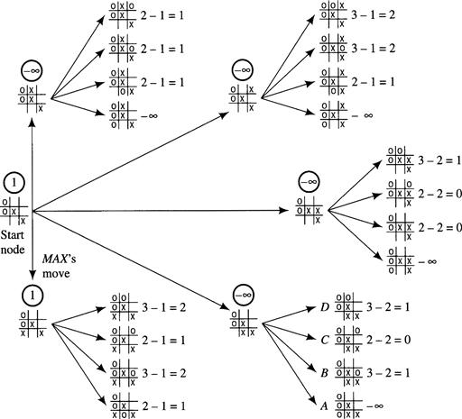
Figure 12.5 The Last Stage of Search in Tic-Tac-Toe
Some of the tip nodes in this tree (for example, the one marked A) represent wins for MIN and thus have evaluations equal to – ∞. When these evaluations are backed up, we see that MAX’s best move is also the only one that avoids his immediate defeat. Now MIN can see that MAX must win on his next move, so MIN gracefully resigns.
12.3 The Alpha-Beta Procedure
The search procedure that I have just described separates completely the processes of search-tree generation and position evaluation. Only after tree generation is completed does position evaluation begin. It happens that this separation results in a grossly inefficient strategy. Remarkable reductions (amounting sometimes to many orders of magnitude) in the amount of search needed (to discover an equally good move) are possible if we perform tip-node evaluations and calculate backed-up values simultaneously with tree generation. The process is similar to alpha pruning discussed in Chapter 10.
Consider the search tree at the last stage of our Tic-Tac-Toe search (Figure 12.5). Suppose that a tip node is evaluated as soon as it is generated. Then after the node marked A is generated and evaluated, there is no point in generating (and evaluating) nodes B, C, and D; that is, since MIN has A available and MIN could prefer nothing to A, we know immediately that MIN will choose A. We can then assign A’s parent the backed-up value of –∞ and proceed with the search, having saved the search effort of generating and evaluating nodes B, C, and D. (Note that the savings in search effort would have been even greater if we were searching to greater depths; for then none of the descendants of nodes B, C, and D would have to be generated either.) It is important to observe that failing to generate nodes B, C, and D can in no way affect what will turn out to be MAX’s best-first move.
In this example, the search savings depended on the fact that node A represented a win for MIN. The same kind of savings can be achieved, however, even when none of the positions in the search tree represents a win for either MAX or MIN.
Consider the first stage of the Tic-Tac-Toe tree shown earlier (Figure 12.3). I repeat part of this tree in Figure 12.6. Suppose that search had progressed in a depth-first manner and that whenever a tip node is generated, its static evaluation is computed. Also suppose that whenever a position can be given a backed-up value, this value is computed. Now consider the situation occurring at that stage of the depth-first search immediately after node A and all of its successors have been generated, but before node B is generated. Node A is now given the backed-up value of –1. At this point, we know that the backed-up value of the start node is bounded from below by –1. Depending on the backed-up values of the other successors of the start node, the final backed-up value of the start node may be greater than –1, but it cannot be less. We call this lower bound an alpha value for the start node.

Figure 12.6 Part of the First Stage of Search in Tic-Tac-Toe
Now let depth-first search proceed until node B and its first successor node, C, are generated. Node C is then given the static value of –1. Now we know that the backed-up value of node B is bounded from above by –1. Depending on the static values of the rest of node B’s successors, the final backed-up value of node B can be less than –1, but it cannot be greater. We call this upper bound on node B a beta value. We note at this point, therefore, that the final backed-up value of node B can never exceed the alpha value of the start node, and therefore we can discontinue search below node B. We are guaranteed that node B will not turn out to be preferable to node A.
This reduction in search effort was achieved by keeping track of bounds on backed-up values. In general, as successors of a node are given backed-up values, the bounds on backed-up values can be revised. But we note that
Because of these constraints, we can state the following rules for discontinuing the search:
1. Search can be discontinued below any MIN node having a beta value less than or equal to the alpha value of any of its MAX node ancestors. The final backed-up value of this MIN node can then be set to its beta value. This value may not be the same as that obtained by full minimax search, but its use results in selecting the same best move.
2. Search can be discontinued below any MAX node having an alpha value greater than or equal to the beta value of any of its MIN node ancestors. The final backed-up value of this MAX node can then be set to its alpha value.
During search, alpha and beta values are computed as follows:
• The alpha value of a MAX node is set equal to the current largest final backed-up value of its successors.
• The beta value of a MIN node is set equal to the current smallest final backed-up value of its successors.
When search is discontinued under rule 1, we say that an alpha cut-off has occurred; when search is discontinued under rule 2, we say that a beta cut-off has occurred. The whole process of keeping track of alpha and beta values and making cut-offs when possible is usually called the alpha-beta procedure. The procedure terminates when all of the successors of the start node have been given final backed-up values, and the best first move is then the one creating that successor having the highest backed-up value. Employing this procedure always results in finding a move that is as good as the move that would have been found by the simple minimax method searching to the same depth. The only difference is that the alpha-beta procedure finds a best first move usually after much less search.
My verbal description of the alpha-beta procedure can be captured by a concise pseudocode recursive algorithm. The following version, which evaluates the minimax value of a node n relative to the cut-off values α and β, is adapted from [Pearl 1984, p. 234]:
AB(n; α, β)
1. If n at depth bound, return AB(n) = static evaluation of n. Otherwise, let n1, …, nk, …, nb be the successors of n (in order), set k ←1 and, if n is a MAX node, go to step 2; else go to step 2’.
We begin an alpha-beta search by calling AB (s; –∞, +∞), where s is the start node. Throughout the algorithm, α < β. The ordering of nodes in step 1 of the algorithm has an important effect on its efficiency, as we shall see.
An application of the alpha-beta procedure is illustrated in Figure 12.7. I show a search tree generated to a depth of 6. MAX nodes are depicted by a square, and MIN nodes are depicted by a circle. The tip nodes have the static values indicated. Now suppose we conduct a depth-first search employing the alpha-beta procedure. (My convention is to generate the bottom-most nodes first.) The subtree generated by the alpha-beta procedure is indicated by darkened branches. Those nodes cut off have X’s drawn through them. Note that only 18 of the original 41 tip nodes had to be evaluated. (You can test your understanding of the procedure by attempting to duplicate the alpha-beta search on this example.)

Figure 12.7 An Example of Alpha-Beta Search
12.4 The Search Efficiency of the Alpha-Beta Procedure
In order to perform alpha and beta cut-offs, at least some part of the search tree must be generated to maximum depth, because alpha and beta values must be based on the static values of tip nodes. Therefore, some type of a depth-first search is usually employed in using the alpha-beta procedure. Furthermore, the number of cut-offs that can be made during a search depends on the degree to which the early alpha and beta values approximate the final backed-up values.
Suppose a tree has depth d, and every node (except a tip node) has exactly b successors. Such a tree will have precisely bd tip nodes. Suppose an alpha-beta procedure generated successors in the order of their true backed-up values—the lowest-valued successors first for MIN nodes and the highest-valued successors first for MAX nodes. (Of course, these backed-up values are not typically known at the time of successor generation, so this order could never really be achieved, except perhaps accidentally.)
It happens that this order maximizes the number of cut-offs that will occur and minimizes the number of tip nodes generated. Let us denote this minimal number of tip nodes by Nd. It can be shown [Slagle & Dixon 1969, Knuth & Moore 1975] that
![]()
That is, the number of tip nodes of depth d that would be generated by optimal alpha-beta search is about the same as the number of tip nodes that would have been generated at depth d/2 without alpha-beta. Therefore, in the same time that search without alpha-beta would stop at a depth bound of d/2, alpha-beta search (with perfect ordering) can proceed to a depth of d. In other words, alpha-beta, with perfect ordering, reduces the effective branching factor from b to approximately ![]() .
.
Of course, perfect node ordering cannot be achieved. (If it could, we wouldn’t need the search process at all.) In the worst case, alpha-beta search produces no cut-offs and thus leaves the effective branching factor unchanged. If the successor nodes are ordered randomly, Pearl has shown that alpha-beta search allows search depth to be increased by approximately 4/3; that is, the average branching factor is reduced to approximately ![]() [Pearl 1982b]. (See [Pearl 1984, Ch. 9] for a thorough analysis with historical commentary.) In practice, if good heuristics are used to order successor nodes, the alpha-beta procedure usually comes close to achieving the optimal reduction in the effective branching factor.
[Pearl 1982b]. (See [Pearl 1984, Ch. 9] for a thorough analysis with historical commentary.) In practice, if good heuristics are used to order successor nodes, the alpha-beta procedure usually comes close to achieving the optimal reduction in the effective branching factor.
The most straightforward method for ordering successor nodes is simply to use the static evaluation function. Another technique for node ordering comes as a side effect of using a version of iterative deepening—first used in the Chess-playing program CHESS 4.5 [Slate & Atkin 1977]. The program first searched to a depth bound of one ply and then evaluated the best move; then it searched all over again to two ply and evaluated the best move; and so on. The main reason for these multiple, and seemingly wasteful, searches is that game-playing programs often have time constraints. Depending on the time resources available, search to deeper plys can be aborted at any time, and the move judged best by the search last completed can be made. The node-ordering side effect comes about because the successors judged to be best in the ply k search can be used to order nodes in the ply k + 1 search.
12.5 Other Important Matters
For most of the game (in most games), search must end before terminating positions are found (limited horizon), causing various difficulties. One difficulty is that search might end at a position in which MAX (or MIN) is able to make a great move. For this reason, most game-searching programs make sure that a position is quiescent before ending search at that position. A position is quiescent if its static value is not much different from what its backed-up value would be by looking a move or two ahead.
Even by insisting on quiescence before ending search along a certain branch, there can be situations in which disaster or success lurks just beyond the search horizon. There are situations in some games that inevitably lead to success for MAX, say, no matter what MIN does, but for which MIN is able to make quiescence-preserving stalling moves that push MAX’s success beyond the search horizon. This so-called horizon effect is one of the primary difficulties facing game-playing programs.
Both the minimax method and its alpha-beta extension assume that the opposing player will always make its best move. There are occasions in which this assumption is inappropriate. Suppose, for example, that MAX is in a situation that appears to be losing—assuming that MIN will play optimally. Yet, there exists a move for MAX that gets it out of its difficulty if only MIN would make a mistake. The minimax strategy won’t recommend such a move, yet (since the game appears lost anyway) there would seem to be little additional risk in gambling that MIN will err. Minimax would also be inappropriate if one player had some kind of model of the other player’s strategy. Perhaps the other “player” is not really an opponent but simply another agent of change.
12.6 Games of Chance
Some games, such as Backgammon, involve an element of chance. For example, the moves that one is allowed to make might depend on the outcome of a throw of the dice. The game tree for a prototypical game of this type is shown schematically in Figure 12.8. (To make the tree somewhat simpler, I show only the six different outcomes possible by throwing a single die.) MAX’s and MIN’s “turns” now each involve a throw of the die. We might imagine that at each dice throw, a fictitious third player, DICE, makes a move. That move is determined by chance. In the case of throwing a single die, the six outcomes are all equally probable, but the chance element could also involve an arbitrary probability distribution.

Figure 12.8 Game Tree for a Game Involving a Dice Throw
Values can be backed up in game trees involving chance moves also, except that when backing up values to nodes at which there is a chance move, we might back up the expected (average) values of the values of the successors instead of a maximum or minimum.3 The numbers adjacent to the nodes in Figure 12.8 are presumed backed-up values. We back up the minimum value of the values of successors of nodes for which it is MIN’s move, the maximum value of the values of successors of nodes for which it is MAX’s move, and the expected value of the values of successors of nodes for which it is the DICE’s move. This modified backing-up procedure is sometimes called expectimaxing.
Introducing a chance move often makes the game tree branch too much for effective searching. In such cases, it is extremely important to have a good static evaluation function so that search does not have to go very deep. If a sufficiently good static evaluation function were available, MAX’s policy for choosing a move could look just at the positions one move ahead and make that move that maximizes the value of the static evaluation function of those positions. In the next section, we discuss techniques for learning action policies and for learning static evaluation functions in games having branching factors too large to permit search.
12.7 Learning Evaluation Functions
Some games (such as Go) allow so many moves at each stage that deep searches would seem not to be feasible.4 Without any search, the best move would have to be selected based just on the static evaluation of the successors or by reacting to the immediate board position through various pattern recognition techniques. In Go, for example, effort has been devoted to finding ways to evaluate and to respond reactively to positions [Zobrist 1970, Reitman & Wilcox 1979, Kierulf, Chen, & Nievergelt 1990].
Sometimes, good static evaluation functions can be learned by neural networks. The game of Backgammon provides an example. A program called TD-GAMMON [Tesauro 1992, Tesauro 1995] learns to play Backgammon by training a layered, feedforward neural network. The structure of the neural net and its coding is as shown in Figure 12.9. The 198 inputs (which represent a Backgammon board situation) are fully connected to the hidden units, and the hidden units are fully connected to the output units. The hidden units and the output units are sigmoids. It is intended that the output units produce estimates, p1, p2, p3, and p4, of the probabilities of various outcomes of the game resulting from any given input board position. The overall value of a board position is then given by an estimated “payoff,” v =p1 + 2p2 – p3 – 2p4. In using the network to play Backgammon, the dice are thrown and the boards permitted by all of the possible moves from the existing board and that dice roll are evaluated by the network. The board with the best value of v is selected, and the move that produces that board is made. (If it is White’s move, the highest value of v is best; if it is Black’s move, the smallest value of v is best.)

Figure 12.9 The TD-GAMMON Network
Temporal difference training of the network is accomplished during actual play using the network to play games against itself. When a move is made, the network weights are adjusted, using backpropagation, to make the predicted payoff from the original position closer to that of the resulting position. For simplicity I explain the method as if it used pure temporal difference learning. (A variant is actually used, but that variant need not concern us here.) If vt is the network’s estimate of the payoff at time t (before a move is made), and vt+1 is the estimate at time t + 1 (after a move is made), the standard temporal difference weight-adjustment rule is
![]()
where Wt is a vector of all weights in the network at time t, and ![]() is the gradient of vt in this weight space. (For a layered, feedforward network, such as that of TD-GAMMON, the weight changes for the weight vectors in each layer can be expressed in the manner described in Chapter 3.) The network is trained so that, for all t, its output, vt, for an input before a move tends toward its output, vt+1, for the input after a move (just as in value iteration). Experiments with this training method have been performed by having the network play many hundreds of thousands of games against itself. (Training runs have involved as many as a million and a half games.)
is the gradient of vt in this weight space. (For a layered, feedforward network, such as that of TD-GAMMON, the weight changes for the weight vectors in each layer can be expressed in the manner described in Chapter 3.) The network is trained so that, for all t, its output, vt, for an input before a move tends toward its output, vt+1, for the input after a move (just as in value iteration). Experiments with this training method have been performed by having the network play many hundreds of thousands of games against itself. (Training runs have involved as many as a million and a half games.)
Performance of a well-trained network is at or near championship level. Based on 40 games played against a version of the program that uses some look-ahead search, Bill Robertie (a former Backgammon world champion) estimates that TD-GAMMON 2.1 plays at a strong master level—extremely close (within a few hundredths of a point) to equaling the world’s best human players [Tesauro 1995].
12.8 Additional Readings and Discussion
Just as puzzles have, games too have been important in refining and testing AI techniques. For example, [Russell & Wefald 1991, Ch. 4] propose and evaluate game-tree search algorithms (MGSS* and MGSS2) that use metalevel computations (involving the expected value of continued search) to prune the search tree in a way that is more efficient than alpha-beta. Berliner’s B* algorithm uses interval bounds [Berliner 1979], which also permit more effective pruning. [Korf 1991] has extended the alpha-beta procedure to multiplayer games.
Instead of using numerical evaluation functions, some work on game playing has favored the use of pattern recognition techniques to decide whether one position is better than or worse than another position. This technique has been employed in programs that play Chess end games [Huberman 1968, Bratko & Michie 1980].
The most successful early work on game playing was that of Arthur Samuel who developed machine learning methods for the game of Checkers (Draughts) [Samuel 1959, Samuel 1967], Samuel’s Checker-playing programs played at near-championship level. Jonathan Schaeffer’s CHINOOK program at the University of Alberta [Schaeffer, et al. 1992, Schaeffer 1997] is now regarded as the world Checkers champion. In 1997, the IBM program, DEEP BLUE, defeated the reigning world Chess champion, Garry Kasparov, in a championship match.
[Newborn 1996] is a book on computer Chess, recounting its history up through the 1996 defeat of DEEP BLUE by Garry Kasparov. For a review of this book plus commentary on the role of Chess as a research platform for AI, see [McCarthy 1997]. McCarthy thinks that Chess programs could perform better with less search if they used more humanlike reasoning methods. He thinks that Chess can again become a ”Drosophila“ for AI if researchers would use it to test knowledge-based reasoning methods.
[Michie 1966] coined the term expectimax and experimented with the technique.
[Lee & Mahajan 1988] have applied reinforcement learning methods to the game of Othello, and [Schraudolph, Dayan, & Sejnowski 1994] have applied temporal difference techniques to the game of Go.
For more on game search methods generally, see [Pearl 1984, Ch. 9].
Exercises
12.1 Why does search in game-playing programs always proceed forward from the current position rather than backward from the goal?
12.2 Consider the following game tree in which the static scores (in parentheses at the tip nodes) are all from the first player’s point of view. Assume that the first player is the maximizing player.

1. What move should the first player choose?
2. What nodes would not need to be examined using the alpha-beta algorithm—assuming that nodes are examined in left-to-right order?
12.3 (Courtesy of Matt Ginsberg.) Suppose that you are using alpha-beta pruning to determine the value of a move in a game tree, and that you have decided that a particular node, n, and its children can be pruned. If the game tree is in fact a graph and there is another path to the node n, are you still justified in pruning this node? Either prove that you are or construct an example that shows that you cannot.
12.4 Most game-playing programs do not save search results from one move to the next. Instead, they usually start completely over whenever it is the machine’s turn to move. Why?
12.5 Comment (in one-half page or less) how you would modify the minimax strategy so that it could be used to select a move for one of the players in a three-person, perfect-information game. (A perfect-information game is one in which each player knows everything about each state of the game. Chess is a perfect-information game, but bridge is not.) Assume that the players, A, B, and C, play in turn. Assume that the game can end either in all players achieving a “draw” or by one of the three players achieving a “win.” Also assume that the game tree cannot be searched to termination, but that evaluations of nonterminal positions must be backed up by some process analogous to the minimax strategy in order to select a move.
1 However, in this case a better representation, which I leave to you to formulate, is based on whether the distance between the robots is even or odd when it is White’s turn to move. Parity is preserved after a pair of moves!
2 In contrast, Schaeffer estimates that the complete game graph for Checkers has only about 1018 nodes [Schaeffer & Lake 1996]. Because MAX has only to show that one of its moves at every ply leads to a solution, a solution tree would thus have about the square root of this number or 109 nodes. Schaeffer and Lake think that flawless machine Checkers play is attainable “in the near future.”
3 Of course, if we want to be very conservative about the outcome of a chance move, we might instead back up the worst value for MAX whenever it is DICE’S move.
4 Human Go players evidently perform searches over isolated subsets of the board, and it may be necessary and feasible for competent programs to do so also.