
8
Uninformed Search
8.1 Formulating the State Space
Many problems of practical interest have search spaces so large that they cannot be represented by explicit graphs. Elaborations of the basic search procedure described in the last chapter are then required. First, we need to be especially careful about how we formulate such problems for search; second, we have to have methods for representing large search graphs implicitly; and, third, we need to use efficient methods for searching such large graphs.
In some planning problems, like the one about block stacking, it is not too difficult to conceive of data structures for representing the different world states and the actions that change them. Typically though, finding representations that result in manageable state-space graphs is difficult. Doing so requires careful analysis of the problem—taking into account symmetries, ignoring irrelevant details, and finding appropriate abstractions. Unfortunately, the task of setting up problems for search is largely an art that still requires human participation.
In addition to problems involving agents stacking blocks, sliding tile problems are often used to illustrate how state-space search is used to plan action sequences. For variety, I will use problems of this sort in this and the next chapter. A typical example is the Fifteen-puzzle, which consists of fifteen tiles set in a four-by-four array—leaving one empty or blank cell into which an adjacent tile can be slid. The task is to find a sequence of tile movements that transforms an initial disposition of tiles into some particular arrangement. The Eight-puzzle is a reduced version, with eight tiles in a three-by-three array. Suppose the object of the puzzle is to slide tiles from the starting configuration until the goal configuration is reached, as shown in Figure 8.1.
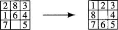
Figure 8.1 Start and Goal Configurations for the Eight-Puzzle
In this problem, an obvious iconic state description would be a three-by-three array in which each cell contains one of the numbers 1 through 8 or a symbol representing the blank space. A goal state is the array representing the configuration on the right side of Figure 8.1. The moves between states correspond to sliding a tile into the blank cell. As mentioned, we often have representational choices in setting up the state space of a problem. In the Eight-puzzle, we might imagine that we have 8 × 4 different moves, namely, move 1 up, move 1 down, move 1 left, move 1 right, move 2 up, …, and so on. (Of course, not all of these moves are possible in any given state.) A more compact formulation involves only four different moves, namely, move blank left, move blank up, move blank right, move blank down. A given start state and the set of possible moves implicitly define the graph of states accessible from the start. The number of nodes in the state-space graph for this representation of the Eight-puzzle is 9! = 362,880. (It happens that the state space for the Eight-puzzle is divided into two separate graphs; a tile configuration in one graph cannot be reached from one in the other graph.)
8.2 Components of Implicit State-Space Graphs
That part of a state-space graph reachable by actions from the start state is represented implicitly by a description of the start state and by descriptions of the effects of actions that can be taken in any state. Thus, it is possible in principle to transform an implicit representation of a graph into an explicit one. To do so, one generates all of the nodes that are successors of the start node (by applying all possible operators at that node), then generates all of their successors, and so on. For graphs that are too large to represent explicitly, the search process need render explicit only so much of the state space as is required to find a path to the goal. The process terminates when an acceptable path to a goal node has been found.
More formally, there are three basic components to an implicit representation of a state-space graph:
1. A description with which to label the start node. This description is some data structure modeling the initial state of the environment.
2. Functions that transform a state description representing one state of the environment into one that represents the state resulting after an action.
These functions are usually called operators. In our agent problems, they are models of the effects of actions. When an operator is applied to a node, it generates one of that node’s successors.
3. A goal condition, which can be either a True-False–valued function on state descriptions or a list of actual instances of state descriptions that correspond to goal states.
We will study two broad classes of search processes. In one, we have no problem-specific reason to prefer one part of the search space to any other, insofar as finding a path to the goal is concerned. Such processes are called uninformed. In the other, we do have problem-specific information to help focus the search. Such processes are called heuristic.1 I begin with the uninformed ones and will discuss heuristic processes in the next chapter.
8.3 Breadth-First Search
Uninformed search procedures apply operators to nodes without using any special knowledge about the problem domain (other than knowledge about what actions are legal ones). Perhaps the simplest uninformed search procedure is breadth-first search. That procedure generates an explicit state-space graph by applying all possible operators to the start node, then applying all possible operators to all the direct successors of the start node, then to their successors, and so on. Search proceeds uniformly outward from the start node. Since we apply all possible operators to a node at each step, it is convenient to group them into a function called the successor function. The successor function, when applied to a node, produces the entire set of nodes that can be produced by applying all of the operators that can be applied to that node. Each application of a successor function to a node is called expanding the node.
Figure 8.2 shows the nodes created in a breadth-first search for a solution to the Eight-puzzle problem. The start and goal nodes are labeled, and the order of node expansions is shown by a numeral next to each node. Nodes of the same depth are expanded according to some fixed order. In expanding a node, I applied operators in the order: move blank left, up, right, down. Even though each move is reversible, I omit the arcs from successors back to their parents. The solution path is shown by the dark line. As we shall see, breadth-first search has the property that when a goal node is found, we have found a path of minimal length to the goal. A disadvantage of breadth-first search, however, is that it requires the generation and storage of a tree whose size is exponential in the depth of the shallowest goal node.
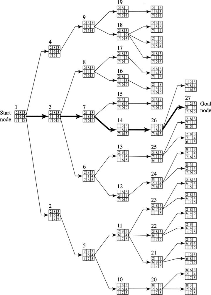
Figure 8.2 Breadth-First Search of the Eight-Puzzle
Uniform-cost search [Dijkstra 1959] is a variant of breadth-first search in which nodes are expanded outward from the start node along “contours” of equal cost rather than along contours of equal depth. If the costs of all arcs in the graph are identical (equal to 1, say), then uniform-cost search is the same as breadth-first search. Uniform-cost search, in turn, can be considered to be a special case of a heuristic search procedure, which I will describe in the next chapter. The brief presentations just given of breadth-first and uniform-cost search methods give the main idea, but they need technical elaboration to cover those cases in which node expansion produces nodes already reached previously by the search process. I defer discussion of these finer points until I deal with the more general algorithm in the next chapter.
8.4 Depth-First or Backtracking Search
Depth-first search generates the successors of a node just one at a time by applying individual operators. A trace is left at each node to indicate that additional operators can eventually be applied there if needed. At each node, a decision must be made about which operator to apply first, which next, and so on. As soon as a successor is generated, one of its successors is generated and so on. To prevent the search process from running away toward nodes of unbounded depth from the start node, a depth bound is used. No successor is generated whose depth is greater than the depth bound. (It is presumed that not all goal nodes lie beyond the depth bound.) This bound allows us to ignore parts of the search graph that have been determined not to contain a sufficiently close goal node.
I illustrate the process using the Eight-puzzle and a depth bound of 5. Again, we apply operators in the order move blank left, up, right, down, and we omit arcs from successors back to their parents. In Figure 8.3a, I show the first few node generations. The number at the left of each node shows the order in which the node is generated; I also show arcs leaving nodes that are not yet fully expanded. At node 5, we reach the depth bound without having reached the goal, so we consider the next most recently generated, but not yet fully expanded node, node 4, and generate the other of its successors, node 6. (See Figure 8.3b.) At this point, we can throw away node 5, since we are not going to generate nodes below it. Node 6 is also at the depth bound and is not a goal node, so we consider the next most recently generated but not fully expanded node, node 2, and generate node 7—throwing away node 3 and its successors since we are not going to generate any more nodes below them. Going back to node 2 is an example of what is called chronological backtracking. When the depth bound is reached again, we have the graph shown in Figure 8.3c. At this point, not having reached a goal node, we generate the other successor of node 8, which is not a goal node either. So, we throw away node 8 and its successors and backtrack to generate another successor of node 7. Continuing this process finally results in the graph shown in Figure 8.4.
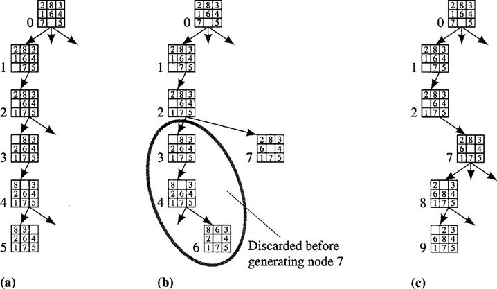
Figure 8.3 Generation of the First Few Nodes in a Depth-First Search

Figure 8.4 The Graph When the Goal Is Reached in Depth-First Search
Note that depth-first search obliges us to save only that part of the search tree consisting of the path currently being explored plus traces at the not yet fully expanded nodes along that path. The memory requirements of depth-first search are thus linear in the depth bound. A disadvantage of depth-first search is that when a goal is found, we are not guaranteed to have found a path to a goal having minimal length. Another problem is that we may have to explore a large part of the search space even to find a shallow goal if it is the only goal and a descendant of a shallow node expanded late in the process.
8.5 Iterative Deepening
A technique called iterative deepening [Korf 1985, Stickel & Tyson 1985] enjoys the linear memory requirements of depth-first search while guaranteeing that a goal node of minimal depth will be found (if a goal can be found at all). In iterative deepening, successive depth-first searches are conducted—each with depth bounds increasing by 1—until a goal node is found. I illustrate how iterative deepening works on a sample tree in Figure 8.5.
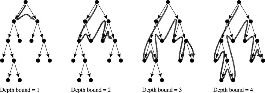
Figure 8.5 Stages in Iterative-Deepening Search
Surprisingly, the number of nodes expanded by iterative-deepening search is not many more than would be expanded by breadth-first search. Let’s calculate this number for the (worst) case of searching a tree with uniform branching factor of b in which the shallowest goal node is at depth d and is the last node to be generated at that depth. The number of nodes expanded by a breadth-first search could be as high as
![]()
To calculate the number of nodes expanded by iterative deepening, we first note that the number of nodes expanded by a complete depth-first search down to level j is
![]()
In the worst case, iterative-deepening search for a goal at depth d has to conduct separate, complete depth-first searches for depths up to d. The sum of the number of nodes expanded for all of these searches is
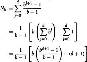
Simplifying yields the total number of nodes that might be expanded by an iterative-deepening search for a goal of depth d:
![]()
For large d, the ratio Nid/Nbf is b/(b – 1). For a branching factor of 10 and deep goals, we expand only about 11% more nodes in an iterative-deepening search than we would in a breadth-first search.
Another, related technique called iterative broadening is useful under certain circumstances when there are many goal nodes. I refer you to [Ginsberg & Harvey 1992, Harvey 1994] for descriptions of this method.
8.6 Additional Readings and Discussion
Various improvements can be made to chronological backtracking. These include dependency-directed backtracking [Stallman & Sussman 1977], backjumping [Gaschnig 1979], and dynamic backtracking [Ginsberg 1993]. The last-cited paper compares these methods and shows the advantages of dynamic backtracking. These enhanced backtracking techniques are usually employed in constraint-satisfaction problems (which will be described in Chapter 11).
Exercises
8.1 In the water-jug puzzle, we are given a 3-liter jug, named Three, and a 4-liter jug, named Four. Initially, Three and Four are empty. Either jug can be filled with water from a tap, T, and we can discard water from either jug down a drain, D. Water may be poured from one jug into the other. There is no additional measuring device. We want to find a set of operations that will leave precisely two liters of water in Four. [Don’t worry! Here’s a solution: (a) fill Three from the tap, (b) pour Three into Four, (c) fill Three from the tap, (d) pour as much from Three into Four as will fill it, (e) discard Four, (f) pour Three into Four.]
1. Set up a state-space search formulation of the water-jug puzzle:
(a) Give the initial iconic state description as a data structure.
(b) Give a goal condition on states as some test on data structures.
(c) Name the operators on states and give precise descriptions of what each operator does to a state description.
2. Draw a graph of all of the distinct state-space nodes that are within three moves of the start node, label each node by its state description, and show at least one path to each node in the graph—labeling each arc by the name of the appropriate operator. In addition to these nodes, show also all of the nodes and arcs (properly labeled) on a path to the solution.
8.2 List the order in which nodes are visited in the tree below for each of the following three search strategies (choosing leftmost branches first in all cases):
2. Depth-first iterative-deepening search (increasing the depth by 1 each iteration)

8.3 Consider a finite tree of depth d and branching factor b. (A tree consisting of only a root node has depth zero; a tree consisting of a root node and its b successors has depth 1; etc.) Suppose the shallowest goal node is at depth g ≤ d.
1. What is the minimum and maximum number of nodes that might be generated by a depth-first search with depth bound equal to d?
2. What is the minimum and maximum number of nodes that might be generated by a breadth-first search?
3. What is the minimum and maximum number of nodes that might be generated by a depth-first iterative-deepening search? (Assume that you start with an initial depth limit of 1 and increment the depth limit by 1 each time no goal is found within the current limit.)
8.4 Assume that 10,000 nodes per second can be generated in a breadth-first search. Suppose also that 100 bytes are needed to store each node. What are the memory and time requirements for a complete breadth-first search of a tree of depth d and branching factor of 5? Show these in a table. (You can use approximate numbers when time is better expressed in hours, days, months, years, etc.)
8.5 Assume we are searching a tree with branching factor b. However, we do not know that we are really searching a tree, so we are considering checking each state description generated to see if it matches a previously generated state description. How many such checks would have to be made in a search of the tree to depth d?
1 The word heuristic comes from the Greek heuriskein, meaning “to discover.” The borrowed phrase Eureka ! (“I have found it!”) comes from the same source.