5
State Machines
5.1 Representing the Environment by Feature Vectors
The feature vector used by an S-R agent can be thought of as representing the state of the environment so far as that agent is concerned. From this feature vector, the S-R agent computes an action appropriate for that environmental state. As I have mentioned, sensory limitations of the agent preclude completely accurate representation of environmental state by feature vectors—especially feature vectors that are computed from immediate sensory stimuli. The accuracy can be improved, however, by taking into account previous sensory history. Important aspects of the environment that cannot be sensed at the moment might have been sensed before. Suppose the agent does have an initial representation of the environment at some time t = 0. (This initial representation might be preloaded by the designer, for example.) We then assume that the representation of environmental state at any subsequent time step, t + 1, is a function of the sensory input at t + 1, the representation of environmental state at the previous time step, t, and the action taken at time t. We call machines that track their environment in this way state machines. Besides immediate sensory inputs, state machines must have memory in which to store a model of the environment.
This model can take many forms. Perhaps the simplest representation is a vector of features—just as is used by S-R machines. But now, the feature vector, Xt +1, depends on a remembered feature vector, Xt. Figure 5.1 illustrates this type of state machine.
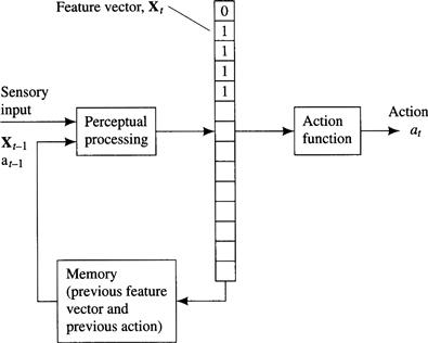
Figure 5.1 A State Machine
Because agent environments might be arbitrarily complex, it is always the case that the agent can only imperfectly represent its environment by a feature vector. But it is also the case that agents designed for specific tasks can afford to conflate many environmental states. The agent designer must arrange for a feature vector that is an adequate representation of the state of the environment—at least insofar as the agent’s tasks are concerned.
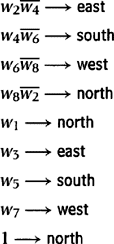
As an example of a state machine, let’s consider our boundary-following robot from Chapter 2. Recall that it modeled its environment by the values of features computed from eight sensory inputs that informed the agent whether or not the eight surrounding cells were free. Let’s consider a somewhat sensory-impaired version of the boundary-following robot. Assume that this robot can sense only the cells immediately to its north, east, south, and west. That is, it cannot sense the four diagonally adjacent cells. Its sensory inputs are (s2, s4, s6, s8), and these inputs have value 1 only if the cells to the north, east, south, and west, respectively, are not free. Otherwise, these inputs have value 0. Even with this impairment, this robot can still perform boundary-following behavior if it computes the needed feature vector from its immediate sensory inputs, the previous feature vector, and the just-performed action. (Again, I assume there are no tight spaces in the environment.)
To follow our practice of making action dependent on a feature vector, we use features wi = si, for i = 2, 4, 6, 8. In place of the four sensory inputs that are absent, we substitute four features, namely, w1, w3, w5, and w7. w1 has value 1 if and only if at the previous time step w2 had value 1 and the robot moved east. Similarly, w3 has value 1 if and only if at the previous time step w4 had value 1 and the robot moved south, and so on. (Otherwise, the wi have value 0.)
Using these features, the following production system gives wall-following behavior (in worlds without tight spaces):
Note that the boundary-following robot of Chapter 2 (without the sensory impairment) managed without memory of previous inputs, features, or actions. If all of the important aspects of the environment can be sensed at the time the agent needs to know them, there is no reason to retain a model of the environment in memory. But sensory abilities are always limited in some way, and thus agents equipped with stored models of the environment will usually be able to perform tasks that memoryless agents cannot.
5.2 Elman Networks
An agent can use a special type of recurrent neural network (called an Elman network [Elman 1990]) to learn how to compute a feature vector and an action from a previous feature vector and sensory inputs. I illustrate how this might be done for the wall-following robot that senses only those four cells to the north, east, south, and west. The network learns to store those properties of previously sensed data that are appropriate to the task at hand. I show such an Elman network in Figure 52. The network has eight hidden units, one for each feature needed by the robot just considered.1 The input to the network consists of the four immediate sensory inputs (s2, s4, s6, s8) plus the values of the eight hidden units one time step earlier. These extra inputs, called context units, allow the network to base its actions on learned properties of data previously sensed—that is, on the context in which the robot currently finds itself. As previously mentioned, there are various ways to arrange for multiple network outputs. In this case, we need four distinguishable outputs, corresponding to the actions north, east, south, and west. The network of Figure 5.2 has four output units, one for each action. Each output unit computes its action from the same set of hidden units (features). We train so that only one output unit has a desired output of 1; the others have desired outputs of 0. Training is accomplished by presenting a sequence of sensory inputs, labeled by the appropriate corresponding actions, that would occur in a typical run of an expert wall-following teacher. In actual operation (after training), we select that action corresponding to the output unit with the largest output. Although an Elman network is a special case of the recurrent neural networks mentioned in Chapter 3, training can be accomplished by ordinary backpropagation because the backward-directed weights (from hidden units to context units) are fixed, and the context units are treated as just another set of inputs.
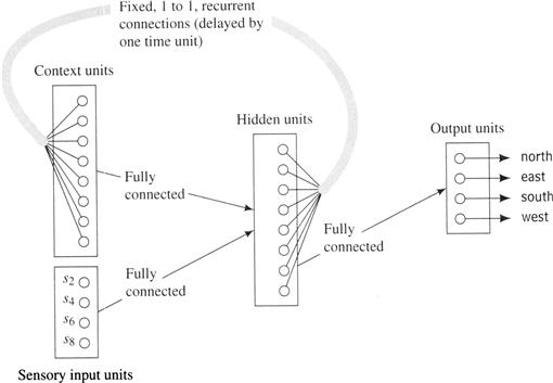
Figure 5.2 An Elman Network
5.3 Iconic Representations
Feature vectors are just one way of representing the environment. Other data structures may also be used. For example, our boundary-following robot might use an array to store a map of free and nonfree cells as it senses them. These two possibilities, representing the world either by features or by data structures, foreshadow a profound division in artificial intelligence. On one side, we have what I call a feature-based representation of the world—a vector of features or attributes. On the other side, we have what I call an iconic representation—data structures such as maps, which can usually be thought of as simulations of important aspects of the environment. (Iconic representations are sometimes also called analogical representations.) A crisp and precise distinction between iconic and feature-based representations is difficult to make, but it is a distinction that we will encounter throughout this book.
When an agent uses an iconic representation, it must still compute actions appropriate to its task and to the present (modeled) state of the environment. Reactive agents react to the data structure in much the same way that agents without memory react to sensory stimuli: they compute features of the data structure. One way to organize such an agent is illustrated in Figure 5.3. The sensory information is first used to update the iconic model as appropriate. Then, operations similar to perceptual processing are used to extract features needed by the action computation subsystem. The actions include those that change the iconic model as well as those that affect the actual environment. The features derived from the iconic model must represent the environment in a manner that is adequate for the kinds of actions the robot must take.

Figure 5.3 An Agent That Computes Features from an Iconic Representation
When the iconic representation of a grid-space robot is a matrix of free and nonfree cells, it is as if the robot had sensors that could sense whether or not any of the cells in the grid were free. For example, consider a robot whose representation of its local environment is as shown in Figure 5.4. Free cells are represented by 0’s in the corresponding array element; nonfree cells are represented by 1’s; unknown cells are represented by ?’s; and the robot’s own location relative to the surrounding cells is represented by the letter R. The environmental situation represented by the array in Figure 5.4 should evoke the action west in a wall-following robot designed to go to the closest wall and then begin wall following. Of course, after taking the action, the robot must update its model to change its own position and to take into account new sensory data.
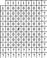
Figure 5.4 A Maplike Iconic Representation
Another type of action computation mechanism uses a model in the form of an artificial potential field. This technique is used extensively in controlling robot motion [Latombe 1991, Ch. 7]. The robot’s environment is represented as a two-dimensional potential field.2 The potential field is the sum of an “attractive” and a “repulsive” component. An attractive field is associated with the goal location—the place that the robot is ordered to go. A typical attractive function is ![]() , where d(X) is the Euclidean distance from a point, X, to the goal. Such a function has minimum value 0 at the goal location. Obstacles in the environment evoke a repulsive field. A typical repulsive function is
, where d(X) is the Euclidean distance from a point, X, to the goal. Such a function has minimum value 0 at the goal location. Obstacles in the environment evoke a repulsive field. A typical repulsive function is ![]() , where d0(X) is the Euclidean distance from X to the closest obstacle point.
, where d0(X) is the Euclidean distance from X to the closest obstacle point.
The total potential is the sum, p = pa + pr. Motion of the robot is then directed along the gradient of the potential field—sliding downhill, so to speak. Either the potential field can be precomputed and stored in memory as an aspect of the world model or it can be computed incrementally at the robot’s location just before the robot needs to decide on a move. An example of a potential field is shown in Figure 5.5. The robot is at the position marked with an R, and the goal location is marked with a G in Figure 5.5a. The attractive, repulsive, and total potentials are shown in Figures 5.5b, c, and d, respectively. Equipotential curves and the path to be followed by the robot are shown in Figure 5.5e. The method suffers from the fact that there can be potential minima that would trap the robot. Several methods have been explored to avoid this problem [Latombe 1991].

5.4 Blackboard Systems
Data structures used to model the world do not necessarily have to be iconic, although they often are. An important style of AI machine is based on a blackboard architecture [Hayes-Roth 1985, Nii 1986a, Nii 1986b], which uses a data structure called a blackboard. The blackboard is read and changed by programs called knowledge sources (KSs). Blackboard systems are elaborations of the production systems I have already described. Each KS has a condition part and an action part. The condition part computes the value of a feature; it can be any condition about the blackboard data structure that evaluates to 1 or 0 (or True or False, if that notation is preferred). The action part can be any program that changes the data structure or takes external action (or both). When two or more KSs evaluate to 1, a conflict resolution program decides which KSs should act. In addition to changing the blackboard, KS actions can also have external effects. And the blackboard might also be changed by perceptual subsystems that process sensory data. Often, the blackboard data structure is organized hierarchically, with subordinate data structures occupying various levels of the hierarchy. I show a schematic of a blackboard system in Figure 5.6.
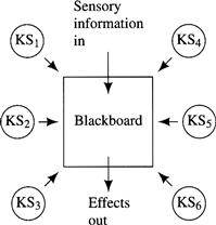
Figure 5.6 A Blackboard System
The KSs are supposed to be “experts” about the part(s) of the blackboard that they watch. When they detect some particular aspect of their part(s) of the blackboard, they propose changes to the blackboard, which, if selected, may evoke other KSs, and so on. Blackboard systems are designed so that as computation proceeds in this manner, the blackboard ultimately becomes a data structure that contains the solution to some particular problem and/or the associated external effects change the world in some desired way. The blackboard architecture has been used in several applications ranging from speech understanding [Erman, et al. 1980], to signal interpretation [Nii 1986b], and medical patient-care monitoring [Hayes-Roth, et al. 1992].
For an example, I return to a robot in grid world—this time our robot can sense all eight cells immediately surrounding it. However, this robot’s sensors (like all real sensors) sometimes give erroneous information. The robot also keeps a partial map of its world—similar to the map shown in Figure 5.4. Because of previous sensor errors, the map can be incomplete and incorrect. The data structure representing the map and a data structure containing sensory data compose the blackboard. I show the blackboard as it appears at one instant of the robot’s experience in Figure 5.7.
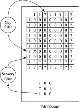
Figure 5.7 A Robot’s Blackboard and KSs
To help the robot correct blackboard errors, it has two KSs, namely, a gap filler and a sensory filter. The gap filler looks for tight spaces in the map, and (knowing that there can be no tight spaces) either fills them in with 1’s or expands them with additional adjacent 0’s. (I leave it to you to speculate about the basis for filling or expanding.) For example, the gap filler decides to fill the tight space at the top of the map in Figure 5.7.
The sensory filter looks at both the sensory data and the map and attempts to reconcile any discrepancies. In Figure 5.7, the sensory filter notes that s7 is a strong “cell-occupied” signal but that the corresponding cell in the map was questionable. It decides to reconcile the difference by replacing that? in the map with a 1. Similarly, it decides that, based on the map data, the s4 = 1 signal is in error and therefore does not alter the map based on this signal. After these actions, the gap filler can replace the lone? in the left-hand column of the map by a 1.
Depending on the task set for the robot, some other KS (reacting to the adjusted map) can propose a robot action.
5.5 Additional Readings and Discussion
State machines are even more ubiquitous than S-R agents. And much of what I said at the end of Chapter 2 about the relationship between S-R agents and ethological models of animal behavior applies also to state machines. Many animals maintain at least partial information about features of their external and internal worlds that cannot be immediately sensed. (See Exercise 5.4.) Production systems that respond to memory as well as to perception have been used to model certain psychological phenomena [Newell 1973].
Elman networks are one example of learning finite-state automata. This problem has also been studied by [Rivest & Schapire 1993].
Many researchers [Kuipers, et al. 1993, Kuipers & Byun 1991] have studied the problem of learning spatial maps, which are examples of iconic representations. When there is uncertainty about the current state and about the effects of actions, map learning is more difficult. This case has been studied by [Dean, Basye, & Kaelbling 1993].
[Genesereth & Nilsson 1987] term agents whose behavior depends on past history hysteretic agents.
Exercises
5.1 A discrete elevator can sense the following information about its world:
1. What floor the elevator is stopped at.
2. What floors passengers in the elevator want to go to.
3. What floors passengers outside of the elevator want rides from and whether they want to go up or down.
4. The status of the elevator door (open or closed).
The elevator is capable of performing the following actions:
1. Go up exactly one floor (unless it is already at the top floor).
2. Go down exactly one floor (unless it is already at the bottom floor).
5. Wait Δ seconds (a fixed time sufficient for all in the elevator to get off and for all outside the elevator to get in).
Design a production system to control the elevator in an efficient manner. (It is not efficient, for example, to reverse the elevator direction from going up to going down either if there is someone still inside the elevator who wants to go to a higher floor or if there is someone outside the elevator who wants to get on from a higher floor.)
5.2 An “artificial ant” lives in a two-dimensional grid world and is able to follow a continuous “pheromone trail” (one cell wide) of marked cells. The ant occupies a single cell and faces either up, left, down, or right. It is capable of five actions, namely, move one cell ahead (m), turn to the left while remaining in the same cell (I), turn to the right while remaining in the same cell (r), set a state bit “on” (on), and set the state bit “off” (off). The ant can sense whether or not there is a pheromone trace in the cell immediately ahead of it (in the direction it is facing), and whether or not the state bit is on. (Assume that the state bit is off initially.) Specify a production system for controlling the ant such that it follows the trail. Assume that it starts in a cell where it can sense a pheromone trace. (Recall that a production system consists of an ordered set of condition-action rules; the action executed is the one that corresponds to the first satisfied condition. A rule might have more than one action on its right-hand side.) Make sure your ant doesn’t turn around and retrace its steps backward!
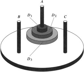
5.3 The three-disc Tower-of-Hanoi puzzle has three pegs, A, B, and C, on which can be placed three discs (labeled D3, D2, and D1) with holes in their centers to fit on the pegs. Disc D3 is larger than disc D2, which is larger than disc D1. Ordinarily, the puzzle has the three pegs in a line, but let’s suppose we position them on a circle. We start with the three discs on peg A and want to move them to one of the other pegs. (See the figure.) The rules are that you can move any disc to any peg except that only the top disc on a peg can be moved, and you cannot place a disc on top of a smaller disc. You might be familiar with a recursive algorithm for solving this problem.
Interestingly, there is another, nonrecursive, algorithm, which can be stated as follows in English: we will always move the largest disc that can be moved, but we will never move it in a direction that undoes the move just previously made. Whenever possible, we move clockwise (CW) on odd-numbered moves and counterclockwise (CCW) on even-numbered moves. When adhering to this CW/CCW schedule is not possible (because there is no such move of the biggest disc that won’t reverse a move just made), we move in the nonpreferred direction instead and then resume the original schedule.
Note: For a simpler algorithm, see www.mkp.com/nils/clarified.
We are going to specify a production system to implement this algorithm. Assume the following six disc-moving actions: move(num, dir), where num can be D3, D2, or D1, and dir can be CW (clockwise) or CCW (counterclockwise). We also assume sensors that can determine the truth or falsity of the following conditions: B1, B2, and B3, where Bi means that disc Di is the largest disc that can be moved. In addition, we will have the following “state” conditions that will be set and unset by the production system: CW (meaning that the last move was clockwise); and M1, M2, and M3, where Mi means that the last disc moved was disc Di. The state-changing actions are toggle, which toggles the state CW (that is, when toggle is executed, CW changes from 1 to 0 or from 0 to 1), and moved(D3), moved(D2), and moved(D1), where moved(Di) sets Mi to true and Mj to false for j ≠ i.
Using these sensory and state conditions and these actions, specify a production system that implements this algorithm. Don’t forget to specify the initial values of the state conditions! Assume that the production system is of the sort in which the production rules are ordered and the action to be executed is the action associated with the highest rule whose condition is satisfied. The action part of a production rule can contain both disc-moving and state-changing actions, which can be executed simultaneously.
5.4 The female solitary wasp, Sphex, lays her eggs in a cricket that she has paralyzed and brought to her burrow nest. The wasp grubs hatch and then feed on this cricket. According to [Wooldridge 1968, p. 70], the wasp exhibits the following interesting behavior:
… the wasp’s routine is to bring the paralyzed cricket to the burrow, leave it on the threshold, go inside to see that all is well, emerge, and then drag the cricket in. If the cricket is moved a few inches away while the wasp is inside making her preliminary inspection, the wasp, on emerging from the burrow, will bring the cricket back to the threshold, but not inside, and will then repeat the preparatory procedure of entering the burrow to see that everything is all right. If again the cricket is removed a few inches while the wasp is inside, once again she will move the cricket up to the threshold and reenter the burrow for a final check…. On one occasion this procedure was repeated forty times, always with the same result.
Invent features, actions, and a production system that this wasp might be using in behaving this way.
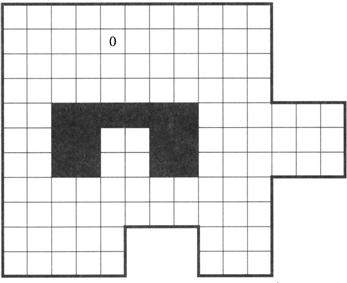
5.5 Invent an artificial potential function (with attractive and repulsive components) that can be used to guide a robot from any cell in the two-dimensional grid world shown here to the goal cell marked by a 0. (Assume that the robot’s possible actions are moves to the north, east, south, and west.) Does the sum of the attractive and repulsive components have local minima? If so, where? Invent a particular overall potential function for this grid world that has no local minima and whose use guarantees shortest paths to the goal.