9. Azure Big Data solutions

In the previous chapter, you learned about the various security strategies that can be implemented on Azure. With a secure application, we manage vast amounts of data. Big data has been gaining significant traction over the last few years. Specialized tools, software, and storage are required to handle it. Interestingly, these tools, platforms, and storage options were not available as services a few years back. However, with new cloud technology, Azure provides numerous tools, platforms, and resources to create big data solutions easily. This chapter will detail the complete architecture for ingesting, cleaning, filtering, and visualizing data in a meaningful way.

The following topics will be covered in this chapter:

• Big data overview
• Data integration
• Extract-Transform-Load (ETL)
• Data Factory
• Data Lake Storage
• Tools ecosystems such as Spark, Databricks, and Hadoop
• Databricks

Big data

With the influx of cheap devices—such as Internet of Things devices and hand-held devices—the amount of data that is being generated and captured has increased exponentially. Almost every organization has a great deal of data and they are ready to purchase more if needed. When large quantities of data arrive in multiple different formats and on an ever-increasing basis, then we can say we are dealing with big data. In short, there are three key characteristics of big data:

• Volume: By volume, we mean the quantity of data both in terms of size (in GB, TB, and PB, for instance) and in terms of the number of records (as in a million rows in a hierarchical data store, 100,000 images, half a billion JSON documents, and so on).
• Velocity: Velocity refers to the speed at which data arrives or is ingested. If data does not change frequently or new data does not arrive frequently, the velocity of data is said to be low, while if there are frequent updates and a lot of new data arrives on an ongoing basis frequently, it is said to have high velocity.
• Variety: Variety refers to different kinds and formats of data. Data can come from different sources in different formats. Data can arrive as structured data (as in comma-separated files, JSON files, or hierarchical data), as semi-structured databases (as in schema-less NoSQL documents), or as unstructured data (such as binary large objects (blobs), images, PDFs, and so on). With so many variants, it's important to have a defined process for processing ingested data.

In the next section, we will check out the general big data process.

Process for big data

When data comes from multiple sources in different formats and at different speeds, it is important to set out a process of storing, assimilating, filtering, and cleaning data in a way that helps us to work with that data more easily and make the data useful for other processes. There needs to be a well-defined process for managing data. The general process for big data that should be followed is shown in Figure 9.1:

Figure 9.1: Big data process

There are four main stages of big data processing. Let's explore them in detail:

• Ingest: This is the process of bringing and ingesting data into the big data environment. Data can come from multiple sources, and connectors should be used to ingest that data within the big data platform.
• Store: After ingestion, data should be stored in the data pool for long-term storage. The storage should be there for both historical as well as live data and must be capable of storing structured, semi-structured, and non-structured data. There should be connectors to read the data from data sources, or the data sources should be able to push data to storage.
• Analysis: After data is read from storage, it should be analyzed, a process that requires filtering, grouping, joining, and transforming data to gather insights.
• Visualize: The analysis can be sent as reports using multiple notification platforms or used to generate dashboards with graphs and charts.

Previously, the tools needed to capture, ingest, store, and analyze big data were not readily available for organizations due to the involvement of expensive hardware and large investments. Also, no platform was available to process them. With the advent of the cloud, it has become easier for organizations to capture, ingest, store, and perform big data analytics using their preferred choice of tools and frameworks. They can pay the cloud provider to use their infrastructure and avoid any capital expenditure. Moreover, the cost of the cloud is very cheap compared to any on-premises solution.

Big data demands an immense amount of compute, storage, and network resources. Generally, the amount of resources required is not practical to have on a single machine or server. Even if, somehow, enough resources are made available on a single server, the time it takes to process an entire big data pool is considerably large, since each job is done in sequence and each step has a dependency upon the prior step. There is a need for specialized frameworks and tools that can distribute work across multiple servers and eventually bring back the results from them and present to the user after appropriately combining the results from all the servers. These tools are specialized big data tools that help in achieving availability, scalability, and distribution out of the box to ensure that a big data solution can be optimized to run quickly with built-in robustness and stability.

The two prominent Azure big data services are HD Insights and Databricks. Let's go ahead and explore the various tools available in the big data landscape.

Big data tools

There are many tools and services in the big data space, and we are going to cover some of them in this chapter.

Azure Data Factory

Azure Data Factory is the flagship ETL service in Azure. It defines incoming data (in terms of its format and schema), transforms data according to business rules and filters, augments existing data, and finally transfers data to a destination store that is readily consumable by other downstream services. It is able to run pipelines (containing ETL logic) on Azure, as well as custom infrastructure, and can also run SQL Server Integration Services packages.

Azure Data Lake Storage

Azure Data Lake Storage is enterprise-level big data storage that is resilient, highly available, and secure out of the box. It is compatible with Hadoop and can scale to petabytes of data storage. It is built on top of Azure storage accounts and hence gets all of the benefits of storage account directly. The current version is called Gen2, after the capabilities of both Azure Storage and Data Lake Storage Gen1 were combined.

Hadoop

Hadoop was created by the Apache software foundation and is a distributed, scalable, and reliable framework for processing big data that breaks big data down into smaller chunks of data and distributes them within a cluster. A Hadoop cluster comprises two types of servers—masters and slaves. The master server contains the administrative components of Hadoop, while the slaves are the ones where the data processing happens. Hadoop is responsible for the logical partition data between slaves; slaves perform all transformation on data, gather insights, and pass them back to master nodes who will collate them to generate the final output. Hadoop can scale to thousands of servers, with each server providing compute and storage for the jobs. Hadoop is available as a service using the HDInsight service in Azure.

There are three main components that make up the Hadoop core system:

HDFS: Hadoop Distributed File System is a file system for the storage of big data. It is a distributed framework that helps by breaking down large big data files into smaller chunks and placing them on different slaves in a cluster. HDFS is a fault-tolerant file system. This means that although different chunks of data are made available to different slaves in the cluster, there is also the replication of data between the slaves to ensure that in the event of any slave's failure, that data will also be available on another server. It also provides fast and efficient access to data to the requestor.

MapReduce: MapReduce is another important framework that enables Hadoop to process data in parallel. This framework is responsible for processing data stored within HDFS slaves and mapping them to the slaves. After the slaves are done processing, the "reduce" part brings information from each slave and collates them together as the final output. Generally, both HDFS and MapReduce are available on the same node, such that the data does not need to travel between slaves and higher efficiency can be achieved when processing them.

YARN: Yet Another Resource Negotiator (YARN) is an important Hadoop architectural component that helps in scheduling jobs related to applications and resource management within a cluster. YARN was released as part of Hadoop 2.0, with many casting it as the successor to MapReduce as it is more efficient in terms of batch processing and resource allocation.

Apache Spark

Apache Spark is a distributed, reliable analytics platform for large-scale data processing. It provides a cluster that is capable of running transformation and machine learning jobs on large quantities of data in parallel and bringing a consolidated result back to the client. It comprises master and worker nodes, where the master nodes are responsible for dividing and distributing the actions within jobs and data between worker nodes, as well as consolidating the results from all worker nodes and returning the results to the client. An important thing to remember while using Spark is that the logic or calculations should be easily parallelized, and the amount of data is too large to fit on one machine. Spark is available in Azure as a service from HDInsight and Databricks.

Databricks

Databricks is built on top of Apache Spark. It is a Platform as a Service where a managed Spark cluster is made available to users. It provides lots of added features, such as a complete portal to manage Spark cluster and its nodes, as well as helping to create notebooks, schedule and run jobs, and provide security and support for multiple users.

Now, it's time to learn how to integrate data from multiple sources and work with them together using the tools we've been talking about.

Data integration

We are well aware of how integration patterns are used for applications; applications that are composed of multiple services are integrated together using a variety of patterns. However, there is another paradigm that is a key requirement for many organizations, which is known as data integration. The surge in data integration has primarily happened during the last decade, when the generation and availability of data has become incredibly high. The velocity, variety, and volume of data being generated has increased drastically, and there is data almost everywhere.

Every organization has many different types of applications, and they all generate data in their own proprietary format. Often, data is also purchased from the marketplace. Even during mergers and amalgamations of organizations, data needs to be migrated and combined.

Data integration refers to the process of bringing data from multiple sources and generating a new output that has more meaning and usability.

There is a definite need for data integration in the following scenarios:

• Migrating data from a source or group of sources to a target destination. This is needed to make data available in different formats to different stakeholders and consumers.
• Getting insights from data. With the rapidly increasing availability of data, organizations want to derive insights from it. They want to create solutions that provide insights; data from multiple sources should be merged, cleaned, augmented, and stored in a data warehouse. 
• Generating real-time dashboards and reports.
• Creating analytics solutions.

Application integration has a runtime behavior when users are consuming the application—for example, in the case of credit card validation and integration. On the other hand, data integration happens as a back-end exercise and is not directly linked to user activity.

Let's move on to understanding the ETL process with Azure Data Factory.

ETL

A very popular process known as ETL helps in building a target data source to house data that is consumable by applications. Generally, the data is in a raw format, and to make it consumable, the data should go through the following three distinct phases:

• Extract: During this phase, data is extracted from multiple places. For instance, there could be multiple sources and they all need to be connected together in order to retrieve the data. Extract phases typically use data connectors consisting of connection information related to the target data source. They might also have temporary storage to bring the data from the data source and store it for faster retrieval. This phase is responsible for the ingestion of data.
• Transform: The data that is available after the extract phase might not be directly consumable by applications. This could be for a variety of reasons; for example, the data might have irregularities, there might be missing data, or there might be erroneous data. Or, there might even be data that is not needed at all. Alternatively, the format of the data might not be conducive to consumption by the target applications. In all of these cases, transformation has to be applied to the data in such a way that it can be efficiently consumed by applications.
• Load: After transformation, data should be loaded to the target data source in a format and schema that enables faster, easier, and performance-centric availability for applications. Again, this typically consists of data connectors for destination data sources and loading data into them.

Next, let's cover how Azure Data Factory relates to the ETL process.

A primer on Azure Data Factory

Azure Data Factory is a fully managed, highly available, highly scalable, and easy-to-use tool for creating integration solutions and implementing ETL phases. Data Factory helps you to create new pipelines in a drag and drop fashion using a user interface, without writing any code; however, it still provides features to allow you to write code in your preferred language.

There are a few important concepts to learn about before using the Data Factory service, which we will be exploring in more detail in the following sections:

• Activities: Activities are individual tasks that enable the running and processing of logic within a Data Factory pipeline. There are multiple types of activities. There are activities related to data movement, data transformation, and control activities. Each activity has a policy through which it can decide the retry mechanism and retry interval.
• Pipelines: Pipelines in Data Factory are composed of groups of activities and are responsible for bringing activities together. Pipelines are the workflows and orchestrators that enable the running of the ETL phases. Pipelines allow the weaving together of activities and allow the declaration of dependencies between them. By using dependencies, it is possible to run some tasks in parallel and other tasks in sequence.
• Datasets: Datasets are the sources and destinations of data. These could be Azure storage accounts, Data Lake Storage, or a host of other sources.
• Linked services: These are services that contain the connection and connectivity information for datasets and are utilized by individual tasks for connecting to them. 
• Integration runtime: The main engine that is responsible for the running of Data Factory is called the integration runtime. The integration runtime is available on the following three configurations:
• Azure: In this configuration, Data Factory runs on the compute resources that are provided by Azure.
• Self-hosted: Data Factory, in this configuration, runs when you bring your own compute resources. This could be through on-premises or cloud-based virtual machine servers.
• Azure SQL Server Integration Services (SSIS): This configuration allows the running of traditional SSIS packages written using SQL Server.
• Versions: Data Factory comes in two different versions. It is important to understand that all new developments will happen on V2, and that V1 will stay as it is, or fade out at some point. V2 is preferred for the following reasons:

  It provides the capability to run SQL Server integration packages.

  It has enhanced functionalities compared to V1.

  It comes with enhanced monitoring, which is missing in V1.

Now that you have a fair understanding of Data Factory, let's get into the various storage options available on Azure.

A primer on Azure Data Lake

Azure Data Lake provides storage for big data solutions. It is specially designed for storing the large amounts of data that are typically needed in big data solutions. It is an Azure-provided managed service. Customers need to bring their data and store it in a data lake.

There are two versions of Azure Data Lake Storage: version 1 (Gen1) and the current version, version 2 (Gen2). Gen2 has all the functionality of Gen1, but one particular difference is that it is built on top of Azure Blob storage.

As Azure Blob storage is highly available, can be replicated multiple times, is disaster-ready, and is low in cost, these benefits are transferred to Gen2 Data Lake. Data Lake can store any kind of data, including relational, non-relational, file system–based, and hierarchical data.

Creating a Data Lake Gen2 instance is as simple as creating a new storage account. The only change that needs to be done is enabling the hierarchical namespace from the Advanced tab of your storage account. It is important to note that there is no direct migration or conversion from a general storage account to Azure Data Lake or vice versa. Also, storage accounts are for storing files, while Data Lake is optimized for reading and ingesting large quantities of data.

Next, we will look into the process and main phases while working with big data. These are distinct phases and each is responsible for different activities on data.

Migrating data from Azure Storage to Data Lake Storage Gen2

In this section, we will be migrating data from Azure Blob storage to another Azure container of the same Azure Blob storage instance, and we will also migrate data to an Azure Data Lake Gen2 instance using an Azure Data Factory pipeline. The following sections outline the steps that need to be taken to create such an end-to-end solution.

Preparing the source storage account

Before we can create Azure Data Factory pipelines and use them for migration, we need to create a new storage account, consisting of a number of containers, and upload the data files. In the real world, these files and the storage connection would already be prepared. The first step for creating a new Azure storage account is to create a new resource group or choose an existing resource group within an Azure subscription.

Provisioning a new resource group

Every resource in Azure is associated with a resource group. Before we provision an Azure storage account, we need to create a resource group that will host the storage account. The steps for creating a resource group are given here. It is to be noted that a new resource group can be created while provisioning an Azure storage account or an existing resource group can be used:

1. Navigate to the Azure portal, log in, and click on + Create a resource; then, search for Resource group.
2. Select Resource group from the search results and create a new resource group. Provide a name and choose an appropriate location. Note that all the resources should be hosted in the same resource group and location so that it is easy to delete them.

After provisioning the resource group, we will provision a storage account within it.

Provisioning a storage account

In this section, we will go through the steps of creating a new Azure storage account. This storage account will fetch the data source from which data will be migrated. Perform the following steps to create a storage account:

1. Click on + Create a resource and search for Storage Account. Select Storage Account from the search results and then create a new storage account.
2. Provide a name and location, and then select a subscription based on the resource group that was created earlier.
3. Select StorageV2 (general purpose v2) for Account kind, Standard for Performance, and Locally-redundant storage (LRS) for Replication, as demonstrated in Figure 9.2:
   

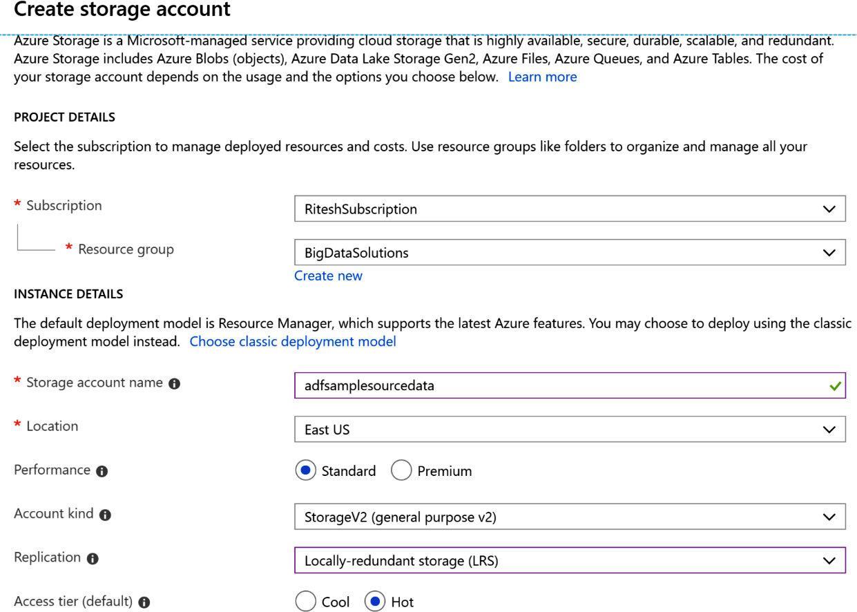
   Figure 9.2: Configuring the storage account

4. Now create a couple of containers within the storage account. The rawdata container contains the files that will be extracted by the Data Factory pipeline and will act as the source dataset, while finaldata will contain files that the Data Factory pipelines will write data to and will act as the destination dataset:
   

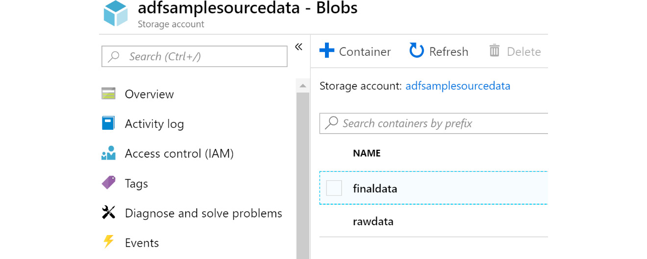
   Figure 9.3: Creating containers

5. Upload a data file (this file is available with the source code) to the rawdata container, as shown in Figure 9.4:
   

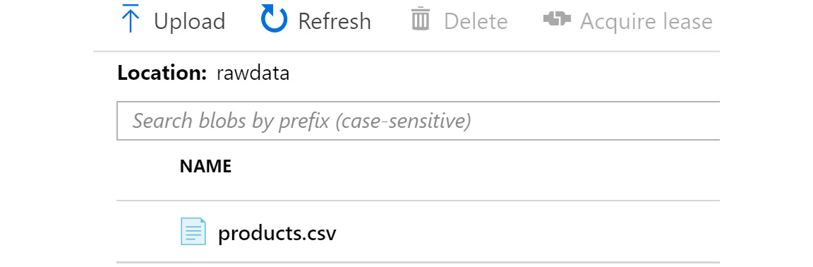
Figure 9.4: Uploading a data file

After completing these steps, the source data preparation activities are complete. Now we can focus on creating a Data Lake instance.

Provisioning the Data Lake Gen2 service

As we already know, the Data Lake Gen2 service is built on top of the Azure storage account. Because of this, we will be creating a new storage account in the same way that we did earlier—with the only difference being the selection of Enabled for Hierarchical namespace in the Advanced tab of the new Azure storage account. This will create the new Data Lake Gen2 service:

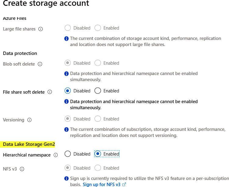
Figure 9.5: Creating a new storage account

After the creation of the data lake, we will focus on creating a new Data Factory pipeline.

Provisioning Azure Data Factory

Now that we have provisioned both the resource group and Azure storage account, it's time to create a new Data Factory resource:

1. Create a new Data Factory pipeline by selecting V2 and by providing a name and location, along with a resource group and subscription selection.

   Data Factory has three different versions, as shown in Figure 9.6. We've already discussed V1 and V2:

   

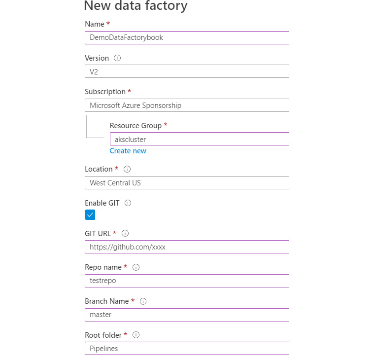
   Figure 9.6: Selecting the version of Data Factory

2. Once the Data Factory resource is created, click on the Author & Monitor link from the central pane.

   This will open another window, consisting of the Data Factory designer for the pipelines.

The code of the pipelines can be stored in version control repositories such that it can be tracked for code changes and promote collaboration between developers. If you missed setting up the repository settings in these steps, that can be done later.

The next section will focus on configuration related to version control repository settings if your Data Factory resource was created without any repository settings being configured.

Repository settings

Before creating any Data Factory artifacts, such as datasets and pipelines, it is a good idea to set up the code repository for hosting files related to Data Factory:

1. From the Authoring page, click on the Manage button and then Git Configuration in the left menu. This will open another pane; click on the Set up code repository button in this pane:
   

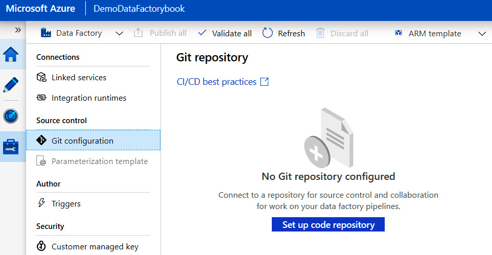
   Figure 9.7: Setting up a Git repository

2. From the resultant blade, select any one of the types of repositories that you want to store Data Factory code files in. In this case, let's select Azure DevOps Git:
   

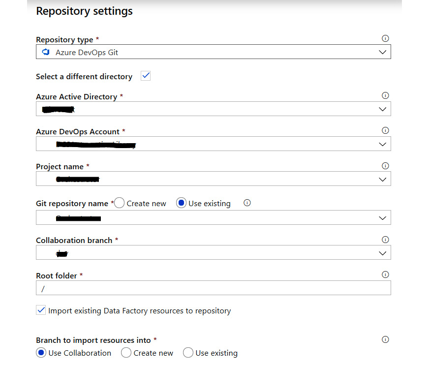
   Figure 9.8: Selecting the appropriate Git repository type

3. Create a new repository or reuse an existing repository from Azure DevOps. You should already have an account in Azure DevOps. If not, visit, https://dev.azure.com and use the same account used for the Azure portal to login and create a new organization and project within it. Refer to Chapter 13, Integrating Azure DevOps, to learn more about creating organizations and projects in Azure DevOps.

   Now, we can move back to the Data Factory authoring window and start creating artifacts for our new pipeline.

In the next section, we will prepare the datasets that will be used within our Data Factory pipelines.

Data Factory datasets

Now we can go back to the Data Factory pipeline. First, create a new dataset that will act as the source dataset. It will be the first storage account that we create and upload the sample product.csv file to:

1. Click on + Datasets -> New DataSet from the left menu and select Azure Blob Storage as data store and delimitedText as the format for the source file. Create a new linked service by providing a name and selecting an Azure subscription and storage account. By default, AutoResolveIntegrationRuntime is used for the runtime environment, which means Azure will provide the runtime environment on Azure-managed compute. Linked services provide multiple authentication methods, and we are using the shared access signature (SAS) uniform resource locator (URI) method. It is also possible to use an account key, service principal, and managed identity as authentication methods:
   

   Figure 9.9: Implementing the authentication method

2. Then, on the resultant lower pane in the General tab, click on the Open properties link and provide a name for the dataset:
   

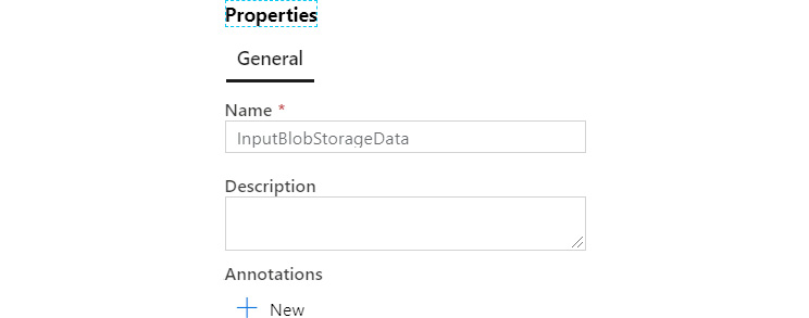
   Figure 9.10: Naming the dataset

3. From the Connection tab, provide details about the container, the blob file name in the storage account, the row delimiter, the column delimiter, and other information that will help Data Factory to read the source data appropriately.

   The Connection tab, after configuration, should look similar to Figure 9.11. Notice that the path includes the name of the container and the name of the file:

   

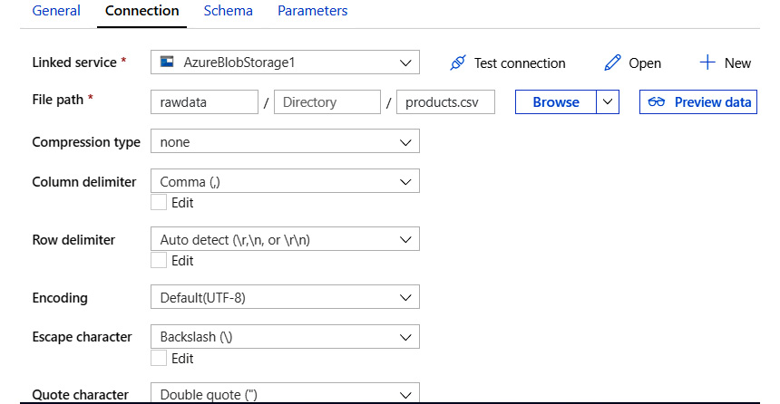
   Figure 9.11: Configuring the connection

4. At this point, if you click on the Preview data button, it shows preview data from the product.csv file. On the Schema tab, add two columns and name them ProductID and ProductPrice. The schema helps in providing an identifier to the columns and also mapping the source columns in the source dataset to the target columns in the target dataset, when the names are not the same.

Now that the first dataset is created, let's create the second one.

Creating the second dataset

Create a new dataset and linked service for the destination blob storage account in the same way that you did before. Note that the storage account is the same as the source but the container is different. Ensure that the incoming data has schema information associated with it as well, as shown in Figure 9.12:

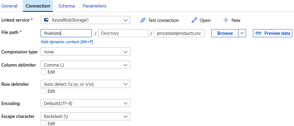
Figure 9.12: Creating the second dataset

Next, we will create a third dataset.

Creating a third dataset

Create a new dataset for the Data Lake Gen2 storage instance as the target dataset. To do this, select the new dataset and then select Azure Data Lake Storage Gen2 (Preview).

Give the new dataset a name and create a new linked service in the Connection tab. Choose Use account key as the authentication method and the rest of the configuration will be auto-filled after selecting the storage account name. Then, test the connection by clicking on the Test connection button. Keep the default configuration for the rest of the tabs, as shown in Figure 9.13:

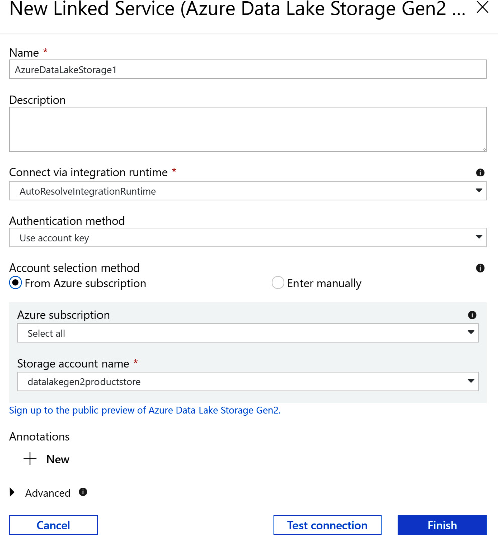
Figure 9.13: Configuration in Connection tabs

Now that we have the connection to source data and also connections to both the source and destination data stores, it's time to create the pipelines that will contain the logic of the data transformation.

Creating a pipeline

After all the datasets are created, we can create a pipeline that will consume those datasets. The steps for creating a pipeline are given next:

1. Click on the + Pipelines => New Pipeline menu from the left menu to create a new pipeline. Then, drag and drop the Copy Data activity from the Move & Transform menu, as demonstrated in Figure 9.14:
   

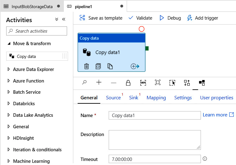
   Figure 9.14: Pipeline menu

2. The resultant General tab can be left as it is, but the Source tab should be configured to use the source dataset that we configured earlier:
   

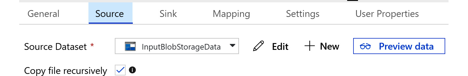
   Figure 9.15: Source tab

3. The Sink tab is used to configure the destination data store and dataset, and it should be configured to use the target dataset that we configured earlier:
   

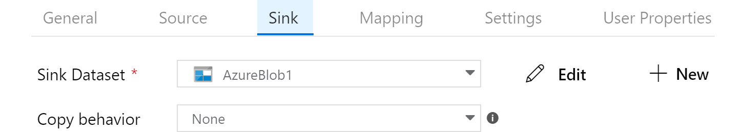
   Figure 9.16: Sink tab

4. On the Mapping tab, map the columns from the source to the destination dataset columns, as shown in Figure 9.17:
   

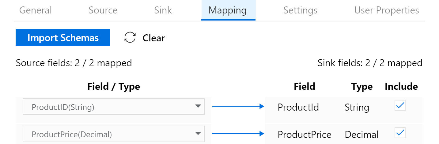
Figure 9.17: Mapping tab

Adding one more Copy Data activity

Within our pipeline, we can add multiple activities, each responsible for a particular transformation task. The task looked at in this section is responsible for copying data from the Azure storage account to Azure Data Lake Storage:

1. Add another Copy Data activity from the left activity menu to migrate data to Data Lake Storage; both of the copy tasks will run in parallel:
   

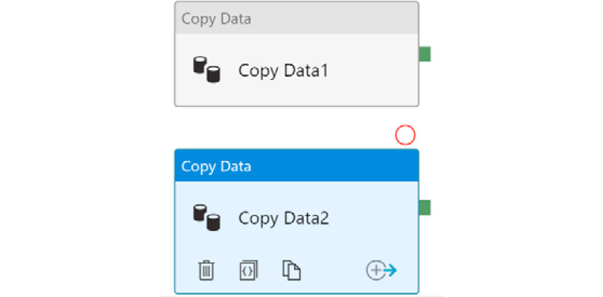
   Figure 9.18: Copy Data activities

   The configuration for the source is the Azure Blob storage account that contains the product.csv file.

   The sink configuration will target the Data Lake Gen2 storage account. 

2. The rest of the configuration can be left in the default settings for the second Copy Data activity.

After the authoring of the pipeline is complete, it can be published to a version control repository such as GitHub.

Next, we will look into creating a solution using Databricks and Spark.

Creating a solution using Databricks

Databricks is a platform for using Spark as a service. We do not need to provision master and worker nodes on virtual machines. Instead, Databricks provides us with a managed environment consisting of master and worker nodes and also manages them. We need to provide the steps and logic for the processing of data, and the rest is taken care of by the Databricks platform.

In this section, we will go through the steps of creating a solution using Databricks. We will be downloading sample data to analyze.

The sample CSV has been downloaded from https://ourworldindata.org/coronavirus-source-data, although it is also provided with the code of this book. The URL mentioned before will have more up-to-date data; however, the format might have changed, and so it is recommended to use the file available with the code samples of this book:

1. The first step in creating a Databricks solution is to provision it from the Azure portal. There is a 14-day evaluation SKU available along with two other SKUs—standard and premium. The premium SKU has Azure Role-Based Access Control at the level of notebooks, clusters, jobs, and tables:
   

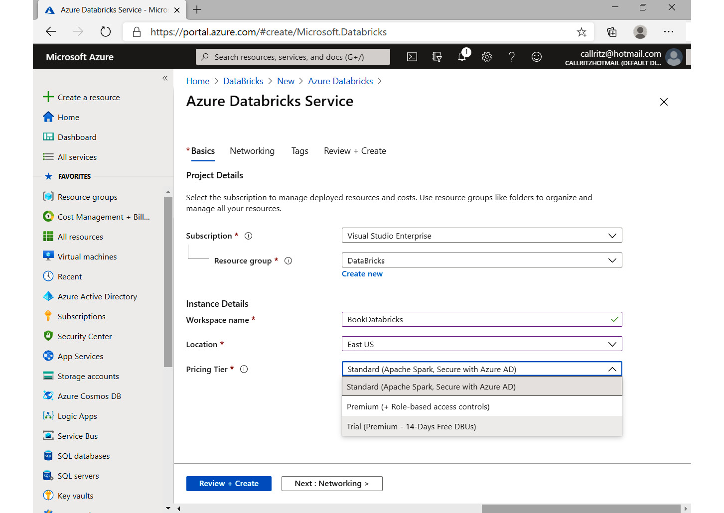
   Figure 9.19: Azure portal—Databricks service

2. After the Data bricks workspace is provisioned, click on the Launch workspace button from the Overview pane. This will open a new browser window and will eventually log you in to the Databricks portal.
3. From the Databricks portal, select Clusters from the left menu and create a new cluster, as shown in Figure 9.20:
   

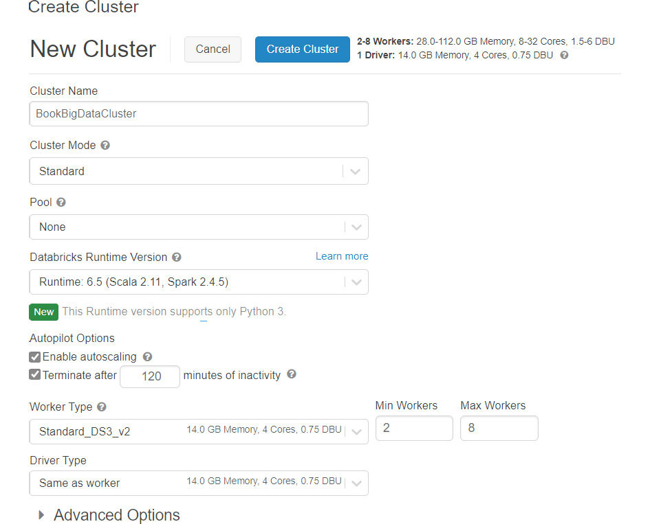
   Figure 9.20: Creating a new cluster

4. Provide the name, the Databricks runtime version, the number of worker types, the virtual machine size configuration, and the driver type server configuration.
5. The creation of the cluster might take a few minutes. After the creation of the cluster, click on Home, select a user from its context menu, and create a new notebook:
   

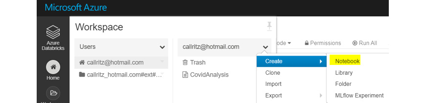
   Figure 9.21: Selecting a new notebook

6. Provide a name to the notebook, as shown next:
   

   Figure 9.22: Creating a notebook

7. Create a new storage account, as shown next. This will act as storage for the raw COVID data in CSV format:
   

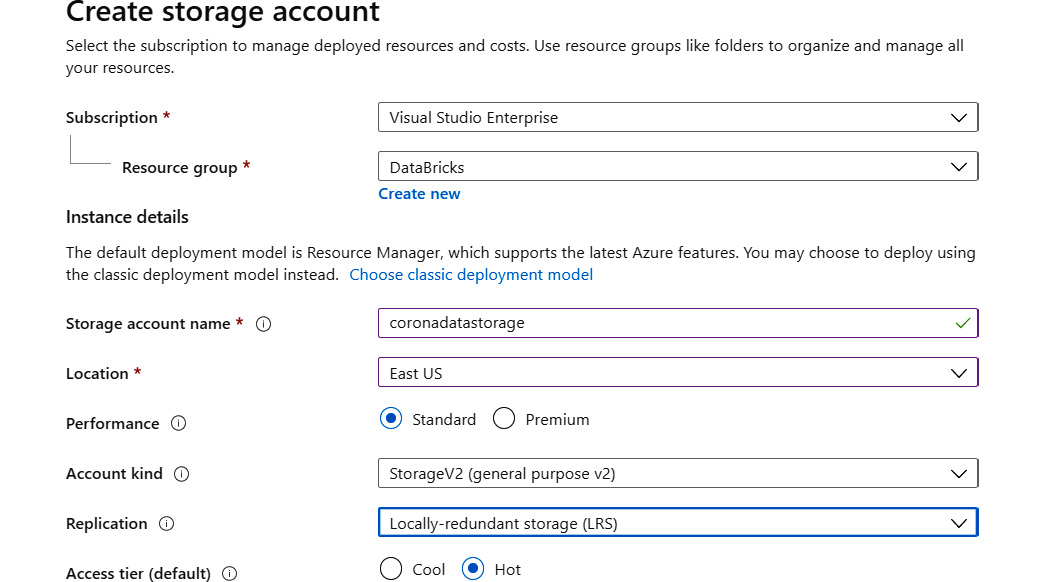
   Figure 9.23: Creating a new storage account

8. Create a container for storing the CSV file, as shown next:
   

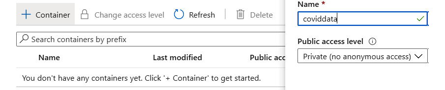
   Figure 9.24: Creating a container

9. Upload the owid-covid-data.csv file to this container.

Once you have completed the preceding steps, the next task is to load the data.

Loading data

The second major step is to load the COVID data within the Databricks workspace. This can be done in two main ways:

• Mount the Azure storage container in Databricks and then load the files available within the mount.
• Load the data directly from the storage account. This approach has been used in the following example.

The following steps should be performed to load and analyze data using Databricks:

1. The first step is to connect and access the storage account. The key for the storage account is needed, which is stored within the Spark configuration. Note that the key here is "fs.azure.account.key.coronadatastorage.blob.core.windows.net" and the value is the associated key:

   spark.conf.set("fs.azure.account.key.coronadatastorage.blob.core.windows.net","xxxxxxxxxxxxxxxxxxxxxxxxxxxxxxxxxxxxxxxxxxxxxxxxxxxxxxxxxxxxxxxxxxxxxxxxxxxxxxxxxxxxxxxxxxxxxxxxxxxxxxxx==")

2. The key for the Azure storage account can be retrieved by navigating to the settings and the Access Keys property of the storage account in the portal.

   The next step is to load the file and read the data within the CSV file. The schema should be inferred from the file itself instead of being provided explicitly. There is also a header row, which is represented using the option in the next command.

   The file is referred to using the following format: wasbs://{{container}}@{{storage account name}}.blob.core.windows.net/{{filename}}.

3. The read method of the SparkSession object provides methods to read files. To read CSV files, the csv method should be used along with its required parameters, such as the path to the CSV file. There are additional optional parameters that can be supplied to customize the reading process of the data files. There are multiple types of file formats, such as JSON, Optimized Row Columnar (ORC), and Parquet, and relational databases such as SQL Server and MySQL, NoSQL data stores such as Cassandra and MongoDB, and big data platforms such as Apache Hive that can all be used within Spark. Let's take a look at the following command to understand the implementation of Spark DataFrames:

   coviddata = spark.read.format("csv").option("inferSchema", "true").option("header", "true").load("wasbs://[email protected]/owid-covid-data.csv")

   Using this command creates a new object of the DataFrame type in Spark. Spark provides Resilient Distributed Dataset (RDD) objects to manipulate and work with data. RDDs are low-level objects and any code written to work with them might not be optimized. DataFrames are higher-level constructs over RDDs and provide optimization to access and work with them RDDs. It is better to work with DataFrames than RDDs.

   DataFrames provide data in row-column format, which makes it easier to visualize and work with data. Spark DataFrames are similar to pandas DataFrames, with the difference being that they are different implementations.

4. The following command shows the data in a DataFrame. It shows all the rows and columns available within the DataFrame:

   coviddata.show()

   You should get a similar output to what you can see in Figure 9.25:

   

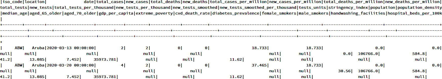
   Figure 9.25: The raw data in a DataFrame

5. The schema of the loaded data is inferred by Spark and can be checked using the following command:

   coviddata.printSchema()

   This should give you a similar output to this:

   

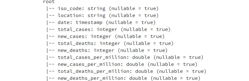
   Figure 9.26: Getting the schema of the DataFrame for each column

6. To count the number of rows within the CSV file, the following command can be used, and its output shows that there are 19,288 rows in the file:

   coviddata.count()

   

   Figure 9.27: Finding the count of records in a DataFrame

7. The original DataFrame has more than 30 columns. We can also select a subset of the available columns and work with them directly, as shown next:

   CovidDataSmallSet = coviddata.select("location","date", "new_cases", "new_deaths")

   CovidDataSmallSet.show()

   The output of the code will be as shown in Figure 9.28:

   

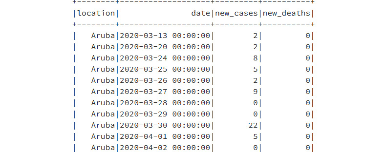
   Figure 9.28: Selecting a few columns from the overall columns

8. It is also possible to filter data using the filter method, as shown next:

   CovidDataSmallSet.filter(" location == 'United States' ").show()

9. It is also possible to add multiple conditions together using the AND (&) or OR (|) operators:

   CovidDataSmallSet.filter((CovidDataSmallSet.location == 'United States') | (CovidDataSmallSet.location == 'Aruba')).show()

10. To find out the number of rows and other statistical details, such as the mean, maximum, minimum, and standard deviation, the describe method can be used:

    CovidDataSmallSet.describe().show()

    Upon using the preceding command, you'll get a similar output to this:

    

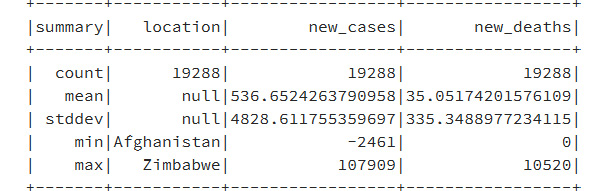
    Figure 9.29: Showing each column's statistics using the describe method

11. It is also possible to find out the percentage of null or empty data within specified columns. A couple of examples are shown next:

    from pyspark.sql.functions import col

    (coviddata.where(col("diabetes_prevalence").isNull()).count() * 100)/coviddata.count()

    The output shows 5.998548320199087, which means 95% of the data is null. We should remove such columns from data analysis. Similarly, running the same command on the total_tests_per_thousand column returns 73.62090418913314, which is much better than the previous column.

12. To drop some of the columns from the DataFrame, the next command can be used:

    coviddatanew=coviddata.drop("iso_code").drop("total_tests").drop("total_tests").drop("new_tests").drop("total_tests_per_thousand").drop("new_tests_per_thousand").drop("new_tests_smoothed").drop("new_tests_smoothed_per_thousand ")

13. At times, you will need to have an aggregation of data. In such scenarios, you can perform the grouping of data, as shown here:

    coviddatanew = coviddata.groupBy('location').agg({'date': 'max'})

    This will display the data from the groupBy statement:

    

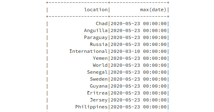
    Figure 9.30: Data from the groupby statement

14. As you can see in the max (date) column, the dates are mostly the same for all the countries, we can use this value to filter the records and get a single row for each country representing the maximum date:

    coviddatauniquecountry = coviddata.filter("date='2020-05-23 00:00:00'")

    coviddatauniquecountry.show()

15. If we take a count of records for the new DataFrame, we get 209.

    We can save the new DataFrame into another CSV file, which may be needed by other data processors:

    coviddatauniquecountry.rdd.saveAsTextFile("dbfs:/mnt/coronadatastorage/uniquecountry.csv")

    We can check the newly created file with the following command:

    %fs ls /mnt/coronadatastorage/

    The mounted path will be displayed as shown in Figure 9.31:

    

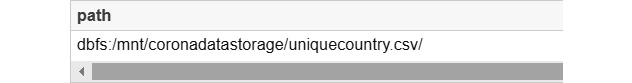
    Figure 9.31: The mounted path within the Spark nodes

16. It is also possible to add the data into the Databricks catalog using the createTempView or createOrReplaceTempView method within the Databricks catalog. Putting data into the catalog makes it available in a given context. To add data into the catalog, the createTempView or createOrReplaceTempView method of the DataFrame can be used, providing a new view for the table within the catalog:

    coviddatauniquecountry.createOrReplaceTempView("corona")

17. Once the table is in the catalog, it is accessible from your SQL session, as shown next:

    spark.sql("select * from corona").show()

    The data from the SQL statement will apear as shown in Figure 9.32:

    

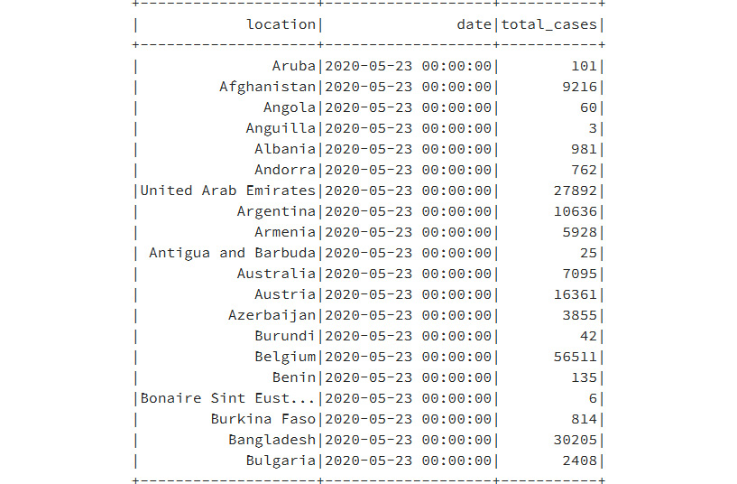
    Figure 9.32: Data from the SQL statement

18. It possible to perform an additional SQL query against the table, as shown next:

    spark.sql("select * from corona where location in ('India','Angola') order by location").show()

That was a small glimpse of the possibilities with Databricks. There are many more features and services within it that could not be covered within a single chapter. Read more about it at https://azure.microsoft.com/services/databricks.

Summary

This chapter dealt with the Azure Data Factory service, which is responsible for providing ETL services in Azure. Since it is a platform as a service, it provides unlimited scalability, high availability, and easy-to-configure pipelines. Its integration with Azure DevOps and GitHub is also seamless. We also explored the features and benefits of using Azure Data Lake Gen2 Storage to store any kind of big data. It is a cost-effective, highly scalable, hierarchical data store for handling big data, and is compatible with Azure HDInsight, Databricks, and the Hadoop ecosystem.

By no means did we have a complete deep dive into all the topics mentioned in this chapter. It was more about the possibilities in Azure, especially with Databricks and Spark. There are multiple technologies in Azure related to big data, including HDInsight, Hadoop, Spark and its related ecosystem, and Databricks, which is a Platform as a Service environment for Spark with added functionality. In the next chapter, you will learn about the serverless computing capabilities in Azure.