
CHAPTER 3
Modifying a Pivot Table
In this chapter, you'll modify the insurance data pivot table you created in Chapter 2 by adding and removing fields and by filtering the pivot table so only specific data is summarized. You'll see what happens when the data in the source table changes, and you'll learn how to view a different type of summary for the values. You'll use a built-in formatting feature to change the appearance of the pivot table, and you'll see how to delete a pivot table if you no longer need it.
By the end of this chapter, I'll have covered the basic of creating and modifying a pivot table. In the remaining chapters, you'll explore the pivot table features in depth so that you fully understand all that a pivot table can do.
To work with the examples in this chapter, you can open the InsurancePolicies03.xlsx file you saved at the end of Chapter 2, or you can download and open the sample file InsurancePolicies03.xlsx.
Changing a Pivot Table
Sometimes you will create a pivot table and leave it in the same layout for many months without changing the fields. Weekly or monthly, you'll update the data, and you'll either review the results or distribute a report based on the pivot table summary.
Other pivot tables will change frequently because you use them to create ad hoc reports, answering the business questions of the day, as you did in Chapter 2 when you analyzed the insurance policy data by region and then by construction type and location. In this chapter, you'll use the same data and pivot table to create more ad hoc reports by using different fields to summarize the data.
Clearing a Pivot Table
There is a threat of flooding in the Midwest region, and you have been asked to report on the insured values in each region for policies with and without flood coverage. You'll clear the contents of the pivot table, and then you'll create a new layout to produce the requested report.
Note You can also remove the existing fields individually by clearing the check boxes in the PivotTable Field List pane.
- Select a cell in the pivot table on Sheet4.
- On the Ribbon, under the PivotTable Tools tab, click the Options tab.
- In the Actions group, click Clear, and then click Clear All (see Figure 3-1).
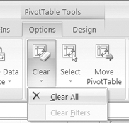
Figure 3-1. Clear the pivot table layout.
- The pivot table layout is cleared of all fields, and only the empty layout is visible on the worksheet. The PivotTable Field List pane has not been cleared and still contains all the fields from the source data.
Adding Fields to Specific Areas of the Pivot Table
In Chapter 2, when you created the pivot table, you checked the fields in the field list, and Excel automatically placed them in the Areas section and in the pivot table layout on the worksheet. Later, you moved a field if you wanted it in a different area.
Instead of accepting the automatic field placement, you can control where the fields are placed. For your flood coverage report, you want regions listed in the Row Labels area and flood coverage listed in the Column Labels area, showing the total insured value for each region and coverage type:
- In the PivotTable Field List pane, add a check mark to the InsuredValue field.
- Because the InsuredValue field contains numeric data, Excel automatically places it in the Values area.
- Add a check mark to the Region field.
- Because Region is a text field, Excel automatically places it in the Row Labels area.
- Next, you want to add the Flood field to the pivot table layout, but you want it in the Column Labels area, not the Row Labels area. In the fields section of the PivotTable Field List pane, drag the Flood field to the Column Labels area (see Figure 3-2).
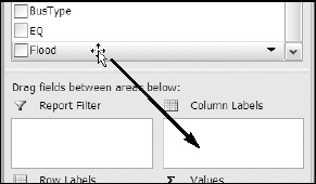
Figure 3-2. Drag a field to the Column Labels area.
- Release the mouse button, and the Flood field appears in the pivot table Column Labels area, showing an N for policies with no coverage and a Y for policies that do have flood coverage.
- To make the numbers easier to read, you can format them. Right-click one of the values in the pivot table, and from the context menu, choose Number Format.
- In the Format Cells dialog box, select the Number category.
- For Decimal Places, select 0, add a check mark for Use 1000 Separator, and then click OK.
With the numbers formatted, you can see that more than $3 million of the insured value is for properties with flood coverage, compared to just $1 million for properties without flood coverage. In the Midwest region, about half of the insured value is for properties with flood coverage.
Adding a Report Filter
You've reported on the overall totals for each region, but the claims manager wants more information. Each policy is for a specific type of business, and your next report should show the total insured value for the manufacturing businesses only. To limit what is included in the summarized data, you'll add a filter to the pivot table by using the BusType field, which stores the business type data.
- In the PivotTable Field List pane, drag the BusType field to the Report Filter area (see Figure 3-3).
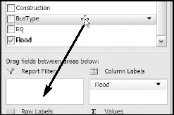
Figure 3-3. Drag a field to the Report Filter area.
- On the worksheet, Excel adds the BusType field to the top of the pivot table, with the item (All) showing (see Figure 3-4). The values in the pivot table have not changed.
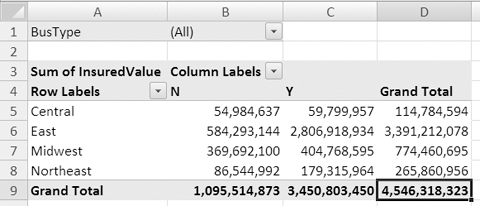
Figure 3-4. The BusType field added to the Report Filter area
- Click the drop-down arrow to the right of (All) to see a list of business types. Each business type from the source data is listed here.
- You'd like to filter the data to see only the manufacturing business types, so click Manufacturing, and click OK (see Figure 3-5).
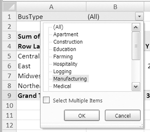
Figure 3-5. Select an item in the Report Filter list.
The values in the pivot table change and now show only the total insured values for policies sold to manufacturing businesses. Of the total insured values in the Midwest region, only $25 million is for manufacturing businesses with flood coverage (see Figure 3-6).
In cell B1 on the worksheet, the drop-down arrow has changed to a filter symbol with a small blue arrow. In the PivotTable Field List pane, there is a filter icon beside BusType in the field list to show that it has a filter applied to that field.
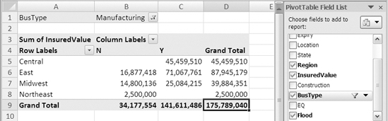
Figure 3-6. A report filter has been applied.
With this filter applied, you can also see that for the manufacturing businesses, all the policies sold in the Central region have flood coverage, but no policies sold in the Northeast region have flood coverage.
Changing the Filter
Now that you have reported on the totals for manufacturing, you're asked to report on the retail businesses in the Midwest. To see the results for a different business type, you can choose a different item from the report filter list.
- Click the arrow for the BusType report filter to open the list of items.
- Click Retail in the list, and click OK.
The pivot table now shows a summary for the retail business type, and of the total insured values in the Midwest region, only $5.7 million is for retail businesses with flood coverage. After reporting on this business type, you can show all the data again.
- To see a summary for all the business types, choose (All) from the top of the report filter list of items.
The pivot table shows the insured values for all business types.
Filtering for Multiple Items
The next report that the claims manager wants is for office buildings and apartments in the Midwest. These are similar types of business, and your report should show a combined total for these. You'll apply a filter to see both Apartment and Office Bldg policies.
- In the pivot table, click the drop-down arrow for the BusType report filter.
- At the bottom of the list, add a check mark next to Select Multiple Items.
- Check boxes appear beside the business type items, and the currently selected item is checked. In your pivot table, (All) is selected, so all the items are checked (see Figure 3-7).
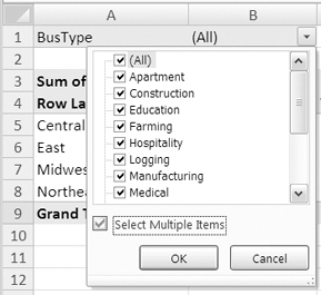
Figure 3-7. You can select multiple items in the Report Filter list.
- To quickly remove the check marks from all the items, click the (All) check box to remove its check mark. This clears all the check marks in the list.
Note Unless at least one item is selected, the OK button will not be available.
- Add check marks to Apartment and Office Bldg. You may have to scroll down the list to see the Office Bldg item by using the scrollbar at the right side of the Report Filter list.
- Click OK to close the list and to apply the filter.
The BusType report filter now shows (Multiple Items), indicating that two or more items have been selected (see Figure 3-8). The pivot table shows the summarized values for the apartment and office building policies, and you can report that most of the insured value is for policies with flood coverage.
Figure 3-8. Multiple items are selected in the Report Filter list.
Removing a Report Filter
If you no longer need a report filter, you can remove it from the pivot table. For now, you're finished analyzing the policies by business type, so you'll remove the report filter:
- Select a cell in the pivot table.
- In the PivotTable Field List pane, remove the check mark from the BusType field name.
The report filter is removed from the pivot table, and the values are a summary of all the records in the source data.
When you remove a filtered field from the pivot table layout, its last setting is remembered. Before removing the BusType field from the pivot table layout, you selected the Apartment and Office Bldg items to filter the pivot table. In the PivotTable Field List pane, the BusType field still shows a filter icon, indicating that the field has a filter applied. Because the field is not in the pivot table layout, the filter currently has no effect on the displayed data.
To see the retained filter, you can examine the BusType field in the PivotTable Field List pane. You will also be able to change the filter settings for the field.
- In the PivotTable Field List, click the BusType field.
- Click the arrow in the field name (see Figure 3-9) to open the field's sort and filter list.
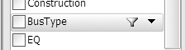
Figure 3-9. Filter icon and arrow in the PivotTable Field List pane
- In the sort and filter list, you can see that the Apartment and Office Bldg items are still checked. The check mark to the left of the filter list indicates that the field has a filter applied (see Figure 3-10).
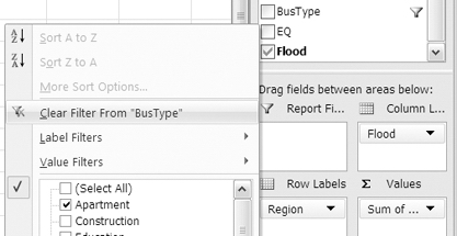
Figure 3-10. Filter and sort list
- Even though the BusType field isn't in the pivot table layout, you can change its filter settings. To remove the filter, click Clear Filter from "BusType" (shown in Figure 3-10).
- The filter and sort list closes, and the filter icon is removed from BusType in the PivotTable Field List pane.
Updating the Pivot Table
After you create a pivot table, it remains connected to the source data. If you make changes to the source data, add new records, or delete records, you can update the pivot table to reflect those changes. In the following sections, you'll make some changes to your source data, and then you'll see the effect of the changes in the pivot table.
Changing the Source Data
You have learned that there is an error in the insured value of one of the policies in the source data, and you have to correct the amount. Also, another policy has been sold, and you must add that information to the source data. You'll go to the Excel table that contains the source data and make the changes:
- A quick way to go to the source data table is to use the Name box, which is located to the left of the Formula Bar, above the worksheet. Click the arrow in the Name box, and in the drop-down list, click Insurance, which is the name of the Excel table that contains the source data (see Figure 3-11).
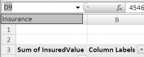
Figure 3-11. Select a name in the Name box.
- Sheet1, where the Excel table is located, is activated, and the entire Excel table is selected. In row 10, for policy 100208, select the InsuredValue ($30,000), which was entered with an incorrect amount.
Note If policy 100208 is not in row 10, you can sort the policies by the policy number in Column A.
- Type the correct entry, which is $3,000,000, and then press the Enter key to complete the correction.
- Next, you'll move to the end of the table and enter a new record. A quick way to move down in a column is to point to the bottom border of the active cell (if it's not a heading cell) and double-click (see Figure 3-12). This will take you to the bottom of the table if there are no blank cells in the active column. Otherwise, it will stop at the cell above the first blank cell.
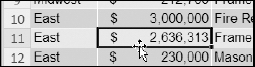
Figure 3-12. Double-click the bottom border of the active cell.
Tip To move down a column using the keyboard, tap the End key and then the down arrow key. This will take you to the bottom of the table if there are no blank cells in the active column. Otherwise, it will stop at the cell above the first blank cell.
- To move to the last column in the last record, double-click the right border of the active cell.
Tip If there is no other data on the worksheet, you can press Ctrl+End to go to the last cell in the table.
- Now that you're in the last cell in the Excel table, press the Tab key to create a new blank record in the table and to move to the first cell in that new record.
- In the Policy column, type an apostrophe and the next available number, as in '101127. The leading apostrophe will force Excel to treat the policy number as text and will ensure that any leading zeroes are retained.
- Press the Tab key to move to the next column, and add the rest of the data for the new record, as shown in Figure 3-13.
Tip To copy a value from the cell above, hold the Ctrl key, and type an apostrophe.

Figure 3-13. New record in the insurance table
- After typing Y in the Flood field, press the Enter key to complete the entry without creating a new record.
Viewing New Data in the Pivot Table
Now that you've completed the changes to your source data, you'll return to the pivot table and update it so you can see the revised summary of the insurance data. You corrected an InsuredValue amount in the East region and added a new policy for the Midwest, so the totals for those regions should increase, as should the grand total.
- Switch to Sheet4, and select any cell in the pivot table. This makes the pivot table active and displays the PivotTable Field List pane.
- On the Ribbon, under the PivotTable Tools tab, click the Options tab.
- In the Data group, click the top section of the Refresh command to update the pivot table with the new and revised data (see Figure 3-14).
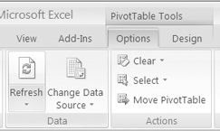
Figure 3-14. The Refresh command in the Data group on the Ribbon
- In the pivot table, the data is refreshed, and it shows new totals for the East and Midwest regions and a new Grand Total amount (see Figure 3-15). For comparison, the old totals are shown in Figure 3-15 but won't remain on your worksheet.
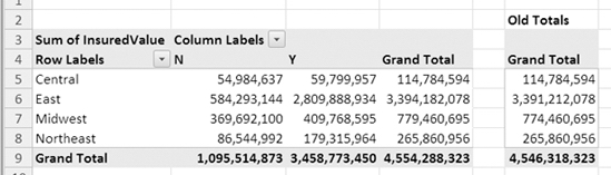
Figure 3-15. The refreshed pivot table shows new totals.
Tip To quickly refresh the pivot table, right-click a cell in the pivot table, and in the context menu, click Refresh.
Changing the Summary Function
Currently, the pivot table shows a Sum of InsuredValue item for each region. Instead of seeing a dollar value, you'd like to know how many policies have been sold in each region for those with flood coverage and for those without. You'll change a setting in the pivot table so you can see a different summary for the InsuredValue field:
- In the pivot table, right-click a cell in the Values area, such as cell C7.
- In the context menu that appears, click Summarize Data By. In the list of functions, the Sum function is checked, because it is the function that is currently used for the InsuredValue field.
- Click Count to summarize the data by that function (see Figure 3-16).
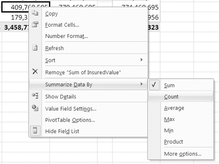
Figure 3-16. Select a different function to summarize the data.
- In the pivot table, the data changes to show a Count of InsuredValue cell instead of a sum (see Figure 3-17). The grand total is 928, which is the number of policy records in the insurance table.
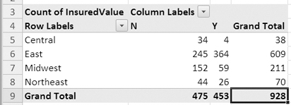
Figure 3-17. The Count of InsuredValue cell
Applying a PivotTable Style
Now that you have set up the summary information the way you want it, you can spend a bit of time on the appearance of the pivot table. Changing the appearance may make the data easier to read, and you may want a color scheme that fits with other documents you're producing.
When you created the pivot table, Excel automatically applied formatting. To quickly change the appearance of the pivot table, you can apply one of the built-in pivot table styles. This may affect the color and font formatting and may add borders and row or column shading.
- Select a cell in the pivot table.
- On the Ribbon, under the PivotTable Tools tab, click the Design tab.
- In the PivotTable Styles group, you can see that one of the styles is selected and has a border around it.
- Point to that style, and its name should appear in a ScreenTip (see Figure 3-18), unless you have turned off the ScreenTip feature.
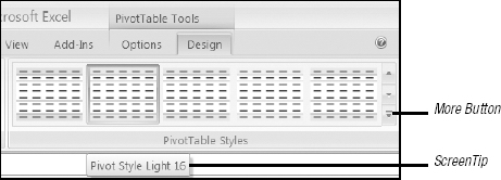
Figure 3-18. Pivot table styles
- Point to one of the other pivot table styles, and the pivot table on the worksheet will show a preview of that style.
- To see other rows of pivot table styles, click the up or down arrow at the right end of the PivotTable Styles group.
- To open the full gallery of pivot table styles, click the More button at the right end of the PivotTable Styles group (shown in Figure 3-18).
- In the gallery, you can drag the scrollbar up and down to see the pivot table styles, which are grouped as Light, Medium, and Dark.
- Point to any pivot table style to see your pivot table previewed with that style. Some styles, such as Pivot Style Medium 2, include horizontal borders and may make the rows easier to follow in a wide pivot table. Some styles have dramatic or dark colors that may be best suited for presentations or online viewing, rather than printing.
Tip If you change your mind and don't want to apply a style, press Esc on the keyboard, or click outside the Style gallery, and it will close without applying a style.
- When you find a pivot table style you like, click it to apply that style to your pivot table.
Note The first style, at the top left of the Light styles, is named None. If you click this style or click the Clear button at the bottom left of the PivotTable Style gallery, your pivot table will not have a style. When no style is applied, the preview function won't work when you point to a different style in the gallery.
Deleting a Pivot Table
A workbook can contain one or more pivot tables, all based on the same data or based on different data. In later chapters, you'll create workbooks with multiple pivot tables and will learn how they interact. Although you can have many pivot tables in the workbook, occasionally you may want to remove a pivot table completely. To practice this technique, you'll delete the pivot table from this workbook:
- Before you delete the pivot table, you can save the workbook to preserve the work you did.
To delete the pivot table, you'll select the entire pivot table, and then delete it.
- Select a cell in the pivot table.
- On the Ribbon, under the PivotTable Tools tab, click the Options tab.
- In the Actions group, click Select, and click Entire PivotTable.
- While the pivot table is selected, press the Delete key on the keyboard. Excel deletes the pivot table from the worksheet, and the PivotTable Field List pane disappears from view.
Tip To immediately restore the pivot table, you can press Ctrl+Z or click the Undo button on the Quick Access Toolbar (QAT), which is located above the Ribbon, beside the Microsoft Office Button.
In some cases, you may want to remove both the pivot table and the worksheet that was inserted when the pivot table was created. If so, you can right-click the worksheet tab, and click Delete in the context menu. When the confirmation message appears, click Delete to permanently remove the worksheet and the pivot table.
Caution You cannot undo the deletion of a worksheet.
- Close the workbook, and do not save the changes when prompted. In the next chapter, you'll use a different workbook with different data.
Summary
In this chapter, you expanded on your basic pivot table skills. You learned how to clear a pivot table and how to add fields to a specific area of the pivot table.
You added a report filter and used it to view summarized data for a specific business type. You changed the report filter and showed data from multiple items from the filter list. When it was no longer needed, you removed the report filter.
Next, you changed data in the source table and added new data, and then you refreshed the pivot table to update its summarized data. You changed the summary function used in the InsuredValue field to use Count instead of Sum.
You applied a pivot table style to make the data in the pivot table easier to read.
Finally, you learned how to delete the entire pivot table from the workbook if required.
I have now covered the basics of creating a pivot table and modifying it. In the remaining chapters, you'll dig deeper into the pivot table features, and you'll see how you can create more sophisticated pivot table reports.