CHAPTER 10

Enhancing Pivot Table
Formatting

Pivot tables are excellent tools for summarizing and presenting data, but sometimes the amount of data they contain is overwhelming. To ensure that the key information is delivered, you can use special formatting features to highlight the most important numbers or to replace the numbers altogether.

In this chapter, you'll use conditional formatting to color cells in a pivot table, and you'll add data bars to illustrate the amounts. You'll also add icons, such as red, yellow, and green traffic lights to indicate progress or decline or to indicate good or poor results. With conditional formatting, you'll color only the values that fall within a specific date range or those that are above or below a certain level.

You'll add other formatting features to your pivot tables to hide or show field items, empty cells, or errors in the pivot table. You can also control the appearance of the pivot table by specifying whether drop-downs, plus signs, and other elements appear.

Applying Conditional Formatting

The safety director wants you to create reports from the company's safety records. The reports will be shared with employees in all the company's locations, and they should present the results clearly and quickly. Instead of creating pivot tables that contain only numbers and headings, you'll use conditional formatting to add visual impact to the data.

Using a Two-Color Scale

Your first report will summarize the safety incidents at each plant location in 2007 and will use color to highlight the locations with the highest and lowest number of incidents. You'll open the file that contains the safety data, create a pivot table, and then add conditional formatting to the values:

1. Download and open the sample file named SafetyData12.xlsx that is available at www.apress.com.

   On Sheet1 is an Excel table that contains safety data, listing the incidents that occurred at each location (see Figure 10-1) from January 2006 to June 2008. The data shows when and where the incident occurred, the type and severity of the incident, and the effects of the incident. The Excel table is named SafetyData, and you'll create a pivot table from this data.

   

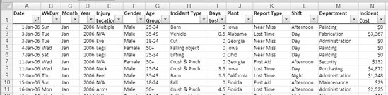
   Figure 10-1. Safety data in an Excel table

2. Select a cell in the Excel table named SafetyData on Sheet1.
3. Create a pivot table on a new worksheet.

   Your first report will show the number of incidents per plant location for 2007, so you'll add those fields to the pivot table and use the Date field to count the records.

4. In the pivot table, add the Plant field to the Row Labels area, add the Year field to the Report Filter area, and add Date to the Values area as Count of Date.
5. In the report filter for Year, select 2007.

The pivot table shows the number of incidents at each location in 2007 and the grand total of 201 (see Figure 10-2).

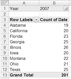
Figure 10-2. Safety incidents per location

To highlight the locations with the highest number of incidents, you'll add conditional formatting. A color scale, with two colors, will use one color for the cell with the highest number and a second color for the cell with the lowest number. Cells with values between the highest and lowest will be shaded in a graduated color scale.

1. Select cells B4 to B12, which contain the location totals you want to color.

---

Caution Do not include the Grand Total cell, or it will be colored as the highest value.

---

1. On the Ribbon, click the Home tab.
2. In the Styles group, click Conditional Formatting (see Figure 10-3).
   
   
   

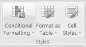
   Figure 10-3. Conditional Formatting command on the Ribbon

3. In the list of conditional formatting options, click Color Scales, and in the second row of Color Scale options, point to the first option, Yellow – Red Color Scale (see Figure 10-4).
   
   
   

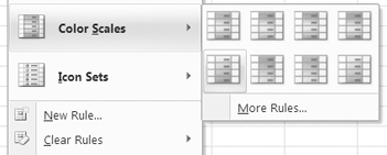
   Figure 10-4. Yellow – Red Color Scale option for conditional formatting

   While pointing to this option, you can see a preview of the formatting on the pivot table. Cell B4, which contains the lowest value, is red, and cell B8, which contains the highest value, is yellow. Red is often associated with danger, so you'd prefer that the highest number be red and the lowest be yellow.

4. In the second row of Color Scale options, point to the second option, Red – Yellow Color Scale. In the formatting preview on the pivot table, the highest number is now red, and the lowest is yellow.
5. Click the Red – Yellow Color Scale option to apply the conditional formatting to the selected cells in the pivot table.

The list of plant locations is now formatted the way you wanted, highlighting the highest and lowest numbers and shading the values in between, in graduated colors from yellow to red. When employees at the locations see the report, they'll quickly recognize which plants have the best and worst results. You can send this report to the safety director and get ready to create the next report.

Removing Conditional Formatting

After applying conditional formatting, you can remove it if it's no longer required. Before starting on your next report, you'll remove the conditional formatting from the pivot table.

1. Select the cells B4 to B12, which contain the cells with conditional formatting.
2. On the Ribbon, click the Home tab, and in the Styles group, click Conditional Formatting.
3. Click Clear Rules, and click Clear Rules from Selected Cells (see Figure 10-5).
   
   
   

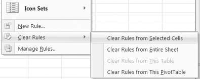
   Figure 10-5. Clear Rules from Selected Cells command

The conditional formatting is removed from the selected cells, and you're ready to start the next report.

Applying a Three-Color Scale

Your next report will summarize the safety incidents in each department per shift in 2007 and will again use color to highlight the locations with the highest and lowest number of incidents. In this report there will be more values, so you'll use a different color scale option. To create the report, you'll change the fields that are in the Row Labels and Column Labels areas.

1. In the pivot table, remove the Plant field from the Row Labels area, add the Department field to the Row Labels area, and add the Shift field to the Column Labels area.

   The pivot table shows the number of incidents per department per shift in 2007, and the grand total remains at 201 (see Figure 10-6).

   

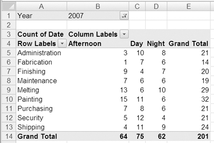
   Figure 10-6. Safety incidents per department per shift

Again to highlight the locations with the highest number of incidents, you'll add color scale conditional formatting. Because this layout has more value cells, you'll use a three-color scale. The cells with the lowest, median, and highest values will be a solid color, and cells with values in between will have a graduated color.

1. Select cells B5 to D13, which contain the values you want to color.

---

Caution Do not include the Grand Total row or column, or these values may be colored as the highest values.

---

1. On the Ribbon, click the Home tab, and in the Styles group, click Conditional Formatting.
2. In the list of conditional formatting options, click Color Scales, and in the first row of Color Scale options, point to the second option, Red – Yellow – Green Color Scale. In the formatting preview on the pivot table, the highest number is now red, the median cells are yellow, and the lowest value is green.
3. Click the Red – Yellow – Green Color Scale option to apply the conditional formatting to the selected cells in the pivot table.

---

Tip Make all the value columns the same width so they appear to be of equal importance in the report.

---

In the report on departments by shift, the afternoon shift in the Painting department is solid red, indicating this is the highest number of incidents. The afternoon shift for Fabrication stands out as the lowest number, since it's solid green. Managers and employees in each department can easily see how their performance compares to other departments. You can send this report to the safety director for distribution and start on the next report.

Using an Icon Set

Instead of color scales, you can use icon sets to illustrate the data. These small pictures will use shapes and colors to mark the values. In your next report, you have been asked to show the change in the number of incidents of each report type from 2006 to 2007. You'll remove two of the fields from the pivot table layout and then add the Report Type field:

1. In the pivot table, remove the Departments field from the Row Labels area, and remove the Shift field from the Column Labels area. Add Report Type to the Row Labels area, and move the Year field to the Column Labels area.
2. Right-click a cell in the Values area, and click Value Field Settings.
3. On the Show Values As tab, choose % Difference From from the Show Values As drop-down list.
4. For the Base field, select Year, and for the Base Item, select (previous).
5. Click Number Format, and format the field as Percentage, with no decimal places.
6. Click OK twice to close the dialog boxes.
7. In the Column Labels drop-down list, remove the check mark from 2008. That year has data for the first six months only, so you don't want to compare it to the other years in this report.
8. Widen column C to about twice its current width, and make column B narrower, since it doesn't contain any values. You can also hide the Grand Total for rows, which is empty.

The pivot table shows the percent difference in the number of incidents per report type from 2006 to 2007 (see Figure 10-7).

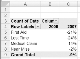
Figure 10-7. Percent difference in incidents per report type

To illustrate the changes in the number of incidents per report type, you'll use an icon set with colored arrows. This will graphically represent the increases, decreases, and lack of change:

1. Select cells C5 to C9, where you want to add icons. For this report you have included the grand total, so its change will also be graphically portrayed.
2. On the Ribbon, click the Home tab, and in the Styles group, click Conditional Formatting.
3. In the list of conditional formatting options, click Icon Sets, and in the first row of Icon Sets options, point to the first option, 3 Arrows (Colored), as shown in Figure 10-8.
   
   
   

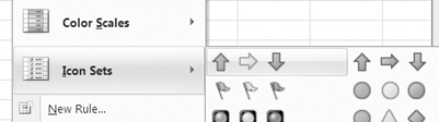
   Figure 10-8. 3 Arrows (Colored) Icon Sets option for conditional formatting

   While pointing to this option, you can see a preview of the formatting on the pivot table. Cells C5 and C6, which contain the lowest values, have a red downward-pointing arrow, and cell C7, which contains the highest value, has a green upward-pointing arrow.

4. Click the 3 Arrows (Colored) Icon Sets option to apply the conditional formatting to the selected cells in the pivot table (see Figure 10-9).
   
   
   

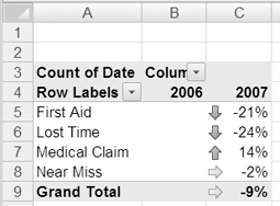
   Figure 10-9. 3 Arrows (Colored) Icon Sets option applied to the pivot table

From your report's numbers and icons, employees will see that first aid and lost time incidents have decreased and medical claims have increased. Near-miss incidents had a slight decrease, and overall, the grand total shows a decrease. You can send this report to the safety director for distribution and start on the next report.

Using Data Bars

The safety director wants a report that shows the number of days lost per month. In this report, you'll have a list of the twelve months and can use conditional formatting to add data bars to the value cells. This will make it easy to visually compare the list of numbers to see which months have the highest number of lost days and which have the fewest.

To start, you'll clear the pivot table to remove the current fields and conditional formatting. Then you'll add the Month field and the Days Lost field, which contains the data on days lost for each incident.

---

Tip You can apply color scales, icon sets, and data bars simultaneously to the cells. However, using more than one of the conditional formatting options may add confusion to the pivot table, rather than help illustrate the data, and using a single type is best in most cases.

---

1. Select a cell in the pivot table, and on the Ribbon, under the PivotTable Tools tab, click the Options tab.
2. In the Actions group, click Clear, and then click Clear All to remove all the fields and formatting from the pivot table layout.
3. Add the Month field to the Row Labels area, and add the Days Lost field to the Values area.
4. Format the Days Lost field as Number, with zero decimal places.

To show which months have the highest number of days lost, you could sort the days in descending order. That would move April and June to the top of the list and put May and September at the bottom. However, you want to keep the months in chronological order, so you'll add data bars to graphically represent the numbers.

1. Select cells B4 to B15, which contain the value cells you want to format. Don't include the Grand Total value, because it is only the individual months you want to compare.
2. On the Ribbon, click the Home tab, and in the Styles group, click Conditional Formatting.
3. In the list of conditional formatting options, click Data Bars, and in the first row of Data Bar options, point to the first option, Blue Data Bar (see Figure 10-10).
   
   
   

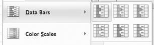
   Figure 10-10. Blue Data Bar option for conditional formatting

   While pointing to this option, you can see a preview of the formatting on the pivot table. Cell B5 has the longest data bar, and cell B12 has the shortest. All the data bar options are identical, except for the color.

4. Click the Blue Data Bar option to apply the conditional formatting to the selected cells in the pivot table (see Figure 10-11).
   
   
   

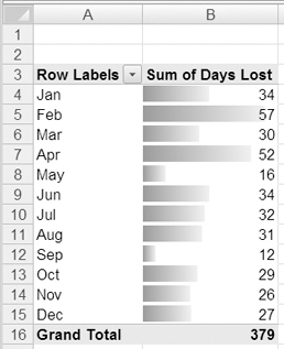
   Figure 10-11. Blue Data Bar option applied to the pivot table

When using data bars, it's important to understand that they aren't exactly like using a bar chart. The data bars are not zero based; the shortest data bar represents the lowest value in the formatted data, and the longest bar represents the highest value in the formatted data. If the lowest value is zero and the highest value is 50, the data bars might look the same as the data bars for data with values that ranged from 500 to 3000 or values from −3000 to −500 (see Figure 10-12). Even if the lowest value is zero or a negative number, it is represented by a small data bar. Later in this chapter you'll learn to change the settings for conditional formatting, and you will be able to adjust how the bars are configured.

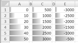
Figure 10-12. Data bars appear the same for widely different values.

If you find it difficult to see where the bars end, because of the graduated coloring in the data bars, you can apply a dark fill color to the cells. For example, in Figure 10-13 the cells have been filled with black, and the number is formatted in a bold six-point font size, with white font color. Column A was made narrower, so the month names are closer to the data bars.

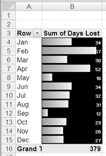
Figure 10-13. Dark fill color in cells with data bars

With the data bars in your report, the safety director can easily compare the number of lost days in the list of months. You can send this report to the safety director and start on the next report.

Formatting Top 10 Items

Pleased with the work you've done so far, the safety director asks for a few more reports. For the next one, the average incident cost should be calculated for each incident type within each age group. The top three amounts should be highlighted, so the safety director can investigate these items further.

To start, you'll clear the pivot table to remove the current fields and conditional formatting. Then you'll add the Age Group field, the Incident Type field, and the Incident Cost field.

1. Select a cell in the pivot table, and on the Ribbon, under the PivotTable Tools tab, click the Options tab.
2. In the Actions group, click Clear, and then click Clear All to remove all the fields and formatting from the pivot table layout.
3. Add the Incident Type field to the Row Labels area, add the Age Group field to the Column Labels area, and add the Incident Cost field to the Values area.
4. Summarize the Incident Cost by Average, and format it as Currency, with zero decimal places.
5. On the Ribbon, under the PivotTable Tools tab, click the Design tab. In the Layout group, click Grand Totals, and then click For Columns Only.

To highlight the amounts that are the top three, you'll use one of the conditional formatting options:

1. Select cells B5 to E13, which contain the value cells you want to format.
2. On the Ribbon, click the Home tab, and in the Styles group, click Conditional Formatting.
3. In the list of conditional formatting options, click Top/Bottom Rules, and then click Top 10 Items (see Figure 10-14).
   
   
   

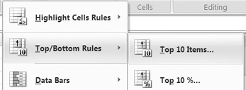
   Figure 10-14. Top 10 Items command in the list of conditional formatting options

   The Top 10 Items dialog box opens, with 10 as the setting in the scroll box on the left. This is similar to the Top 10 feature you used when filtering in the pivot table. The formatting option, Light Red Fill with Dark Red Text, is selected in the drop-down list on the right. The pivot table shows a preview of this formatting, and you'll change the settings to meet your requirements.

4. In the scroll box, change the number of items to 3, and then click the arrow to open the formatting drop-down list (see Figure 10-15).
   
   
   

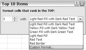
   Figure 10-15. Top 10 Items dialog box

   There is a limited selection of formatting options and none you want to use, so you'll create a custom format of orange fill and bold, black text.

5. In the formatting list, click Custom Format to open thes Format Cells dialog box.
6. On the Font tab, select the Bold font style, and select Black from the Color drop-down list.

---

Note Some formatting options, such as font size or thick borders, are not available, because conditional formatting doesn't allow settings that could affect the cell size.

---

1. On the Fill tab, select Orange as the fill color, and then click OK to close the Format Cells dialog box.
2. Click OK to close the Top 10 Items dialog box.
3. The colors don't display correctly while the cells are selected, so select a cell that is not one of the formatted top three to see the effects of the conditional formatting (see Figure 10-16).
   
   
   

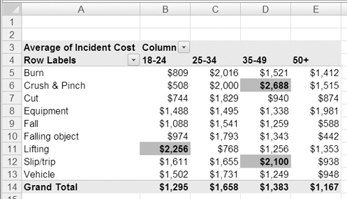
   Figure 10-16. Top three items highlighted

---

Note In the case of a tie, more than the specified number of cells can be formatted.

---

With the Top 10 Items formatting in your report, the safety director can easily identify the items for further investigation. You can send this report to the safety director and start on the next report.

Formatting Cells Between Two Values

The safety director found the Top 10 Items report to be helpful and asks whether you can highlight a few more amounts in that report. Any amount that is between 1,500 and 2,000 should be blue to stand out from the other amounts.

You won't make any changes to the pivot table layout but will add another conditional formatting option to the value cells. To make this formatting more flexible, you'll type the minimum and maximum amounts on the worksheet and refer to those cells in the conditional formatting.

1. In cell G1 on the worksheet, type 1500, which is the minimum amount for the conditional formatting.
2. In cell H1 on the worksheet, type 2000, which is the maximum amount for the conditional formatting.
3. Select cells B5 to E13, which contain the value cells you want to format.
4. On the Ribbon, click the Home tab, and in the Styles group, click Conditional Formatting.
5. In the list of conditional formatting options, click Highlight Cells Rules, and then click Between (see Figure 10-17).
   
   
   

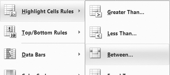
   Figure 10-17. Highlight Cells Rules command in the conditional formatting options

   The Between dialog box opens, with default values in the minimum and maximum boxes. The default formatting option, Light Red Fill with Dark Red Text, is selected in the drop-down list on the right. The pivot table shows a preview of this formatting, and you'll change the settings to meet your requirements.

6. Delete the default value in the minimum box, and click cell G1, which contains the minimum value you typed on the worksheet. Delete the default value in the maximum box, and click cell H1, which contains the minimum value you typed on the worksheet (see Figure 10-18).
   
   
   

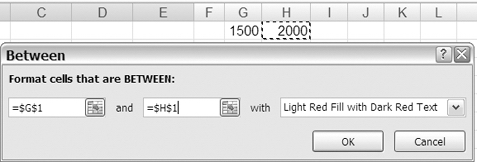
   Figure 10-18. Refer to worksheet cells in the Between dialog box.

7. In the formatting list, click Custom Format to open the Format Cells dialog box.

---

Note In some drop-down lists, such as the formatting list in the Between dialog box, the drop-down list closes automatically when you release the mouse button or when you point with your cursor outside the list. To select an item in this type of list, point to the item, and then release the mouse button. In other lists you may have to click an item to select it and to close the list.

---

1. On the Fill tab, select blue as the fill color, and then click OK to close the Format Cells dialog box.
2. Click OK to close the Between dialog box.
3. The top three cells are still highlighted with orange fill and bold text, and cells with a value between 1,500 and 2,000 are now blue (see Figure 10-19).
   
   
   

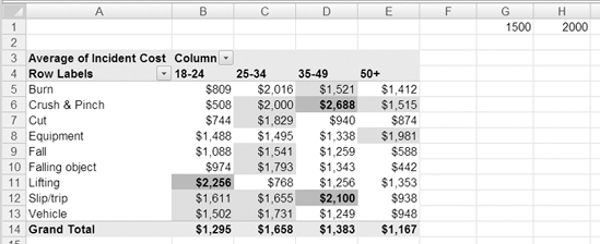
   Figuer 10-19. Two conditional formatting options applied

4. To test the maximum limit, in cell H1 type 1800 as the new limit.

When you press the Enter key to complete the change, the conditional formatting in the pivot table changes to match the new limit.

The safety director will now be able to highlight any range of values simply by changing the amounts in cells G1 and H1. You can send this report to the safety director and start on the next report.

Formatting Labels in a Date Period

The safety director wants some statistics for an education program on preventing injuries, and she has asked whether you can create a report that shows the number of slip/trip injuries during each shift for the current quarter. If possible, any incidents from the current month should be highlighted.

To start, you'll clear the pivot table to remove the current fields and conditional formatting. Then you'll add the Date field, the Incident Type field, and a field to use for counting the incidents.

1. Select a cell in the pivot table, and on the Ribbon, under the PivotTable Tools tab, click the Options tab.
2. In the Actions group, click Clear, and then click Clear All to remove all the fields and formatting from the pivot table layout.
3. Clear cells G1 and H1, which won't be needed for this report.
4. You want to limit the data that's shown in the pivot table, so add the Incident Type field to the Report Filter area, and select Slip/Trip from the Incident Type drop-down list.
5. Add the Date field to the Row Labels area, add the Shift field to the Column Labels area, and add the Report Type field to the Values area, where it will become Count of Report Type.
6. The report should show the incidents from the current quarter, so click the Row Labels arrow, then click Date Filters, and finally click This Quarter.

The results you see will depend on the date you create the report. In this example, the report was created in June 2008 (see Figure 10-20).

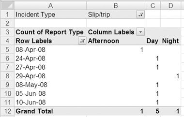
Figure 10-20. Report labels filtered for last quarter

1. In this report, you have been asked to highlight the dates from the current month, so select cells A5 to A11, which contain the date labels you want to format.
2. On the Ribbon, click the Home tab, and in the Styles group, click Conditional Formatting.
3. In the list of conditional formatting options, click Highlight Cells Rules, and then click A Date Occurring (see Figure 10-21).
   
   
   

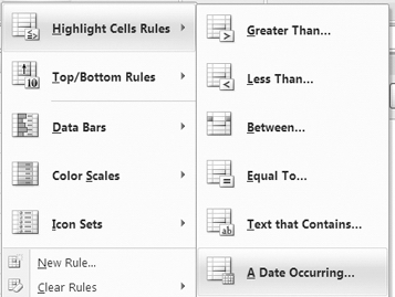
   Figure 10-21. A Date Occurring option in conditional formatting options

   The A Date Occurring dialog box opens, with Yesterday as the setting in the drop-down list at the left. The formatting option, Light Red Fill with Dark Red Text, is selected in the drop-down list at the right. You'll change the settings to meet your requirements.

4. In the date range drop-down list, select This Month Figure 10-22).
   
   
   

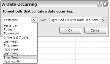
   Figure 10-22. A Date Occurring dialog box

5. Leave the formatting option as the default fill and text, and click OK to close the A Date Occurring dialog box.

The dates from the current month are highlighted and will stand out in the report that you send to the safety director (see Figure 10-23). Because both the date filter (This Quarter) and conditional formatting (This Month) are dynamic, the visible results and highlighting may change the next time the pivot table is refreshed.

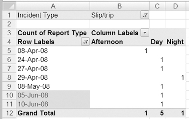
Figure 10-23. Dates from last month are highlighted.

You can send this report to the safety director and start on the next report.

Editing a Rule for Data Bars

The Texas plant has the highest number of days lost, and the safety director wants a report that shows the number of days lost, based on the weekday on which the incident occurred, using data bars instead of numbers. To create an accurate set of data bars, without numbers, you'll use one of the existing Data Bars options and then edit it.

To start, you'll clear the pivot table to remove the current fields and conditional formatting. Then you'll add the WkDay field, which stores the name of the weekday, the Plant field, and the Days Lost field.

1. Select a cell in the pivot table, and on the Ribbon, under the PivotTable Tools tab, click the Options tab.
2. In the Actions group, click Clear, and then click Clear All to remove all the fields and formatting from the pivot table layout.
3. Add the WkDay field to the Row Labels area, and add the Days Lost field to the Values area. The WkDay field will be sorted by weekday, starting with Sunday or Monday.
4. Add the Plant field to the Report Filter area, and filter for Texas, so only the days lost at that plant are showing.

The pivot table shows the days lost for each weekday for the Texas plant. The days range from 4.5 for Sunday, Tuesday, and Thursday to 14.5 for Monday. You'll apply one of the conditional formatting Data Bars options and then modify it to remove the numbers from the cells.

1. Select cells B4 to B10, which contain the value cells you want to format.
2. On the Ribbon, click the Home tab, and in the Styles group, click Conditional Formatting.
3. Click Data Bars, and click Orange Data Bar.

The data bars appear in the cells, with the shortest bars in the three days with 4.5 days lost and the longest bar in Monday (see Figure 10-24). Currently, the bars are distorting the data, because the shortest bar represents the lowest value. Although the lowest number, 4.5, is approximately one half of 9.5, its bar appears to be about one quarter the length of the 9.5 bar.

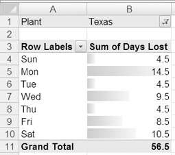
Figure 10-24. Data bars and numbers

Because you will be removing the numbers, it will be important that the data bars reflect the number of days lost as accurately as possible. You'll modify the conditional formatting to remove the numbers and to fix the scale of the data bars.

1. Select cells B4 to B10, which contain the formatted value cells.
2. On the Ribbon, click the Home tab, and in the Styles group, click Conditional Formatting. Then click Manage Rules (see Figure 10-25).
   
   
   

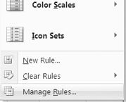
   Figure 10-25. Manage Rules option

The Conditional Formatting Rules Manager dialog box opens, where you can see the Data Bar rule you created when you applied conditional formatting to the Days Lost cells (see Figure 10-26). You'll select that rule and then edit it.

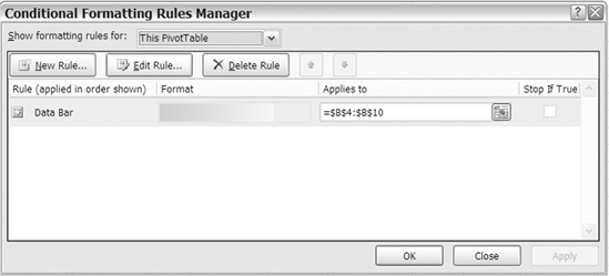
Figure 10-26. Conditional Formatting Rules Manager dialog box

1. In the list of rules, click your Data Bar rule.
2. Click the Edit Rule button to open the Edit Formatting Rule dialog box (see Figure 10-27).
   
   
   

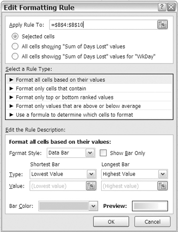
   Figure 10-27. Edit Formatting Rule dialog box

The top section of the Edit Formatting Rule dialog box shows where the rule is applied. The second section shows the type of rule that has been applied. In the third section, Edit the Rule Description, you can see the current settings for the Data Bar rule, and this is where you'll edit the rule. No changes will be required in the first or second section.

1. You want to remove the numbers from the cells, so in the third section, add a check mark to Show Bar Only.

   Currently, the shortest bar represents the lowest value in the range of cells, and this affects the scale of the data bars and exaggerates the differences between numbers. You want to ensure that the amounts are accurately represented in the data bars, so you'll change the settings for Shortest Bar. Instead of using the lowest value in the range of cells, you'll use zero as the setting for Shortest Bar.

2. Click the arrow for the Type drop-down list under Shortest Bar (see Figure 10-28).
   
   
   

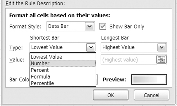
   Figure 10-28. Type options for Shortest Bar

3. Click Number, and a zero automatically appears in the Value box for Shortest Bar. This is the setting you want, so leave Value as zero.
4. Click OK to close the Edit Formatting Rule dialog box, and click OK to close the Conditional Formatting Rules Manager dialog box.

The numbers have been removed from the cells, and the data bars use a scale from zero to the highest number to show a more accurate representation of the numbers. In Figure 10-29 the revised data bars are on the right, and the original data bars are on the left. Fill color was added to make the end of the data bars stand out more clearly.

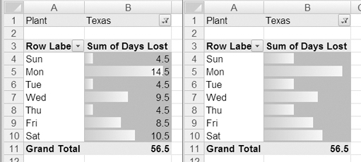
Figure 10-29. Original data bars (left) compared to revised data bars (right)

With the data bars revised to more accurately show the lost days per weekday, you can send this report to the safety director and start on the next report.

Changing the Order of Rules

The next report that the safety director needs is a summary of incident costs per year for each injury location, such as head or back. The top three costs should be highlighted, and any cost that is above average should also be highlighted using a different color.

To start, you'll clear the pivot table to remove the current fields and conditional formatting. Then you'll add the Injury Location field, the Year field, and the Incident field.

1. Select a cell in the pivot table, and on the Ribbon, under the PivotTable Tools tab, click the Options tab.
2. In the Actions group, click Clear, and then click Clear All to remove all the fields and formatting from the pivot table layout.
3. Add the Injury Location field to the Row Labels area, add Year to the Column Labels area, and add the Incident Cost field to the Values area. Format the values as Currency with zero decimal places.
4. Because 2008 is not completed, its values will skew the average, so you'll remove it from the pivot table layout. Click the drop-down arrow for the Column Labels, and remove the check mark for 2008.

First you'll apply conditional formatting to add red fill color to the top three costs:

1. Select cells B5 to C16, which contain the value cells you want to format.
2. On the Ribbon, click the Home tab, and in the Styles group, click Conditional Formatting.
3. In the list of conditional formatting options, click Top/Bottom Rules, and then click Top 10 Items.
4. In the scroll box, change the number of items to 3, and then click the arrow to open the formatting drop-down list.
5. In the formatting list, click Custom Format to open the Format Cells dialog box.
6. On the Fill tab, select a shade of red as the fill color, and then click OK to close the Format Cells dialog box.
7. Click OK to close the Top 10 Items dialog box.

The top three costs are highlighted with red fill (see Figure 10-30). Next, you'll apply conditional formatting so the cells with above average costs are highlighted with yellow fill color.

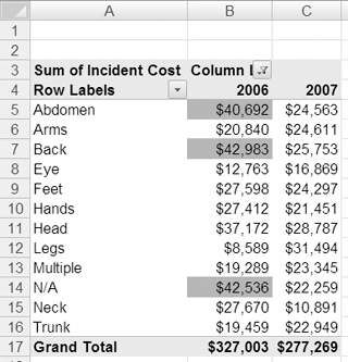
Figure 10-30. The top three items are highlighted with conditional formatting.

1. Select cells B5 to C16, which contain the value cells you want to format.
2. On the Ribbon, click the Home tab, and in the Styles group, click Conditional Formatting.
3. In the list of conditional formatting options, click Top/Bottom Rules, and then click Above Average.
4. In the formatting list, click Custom Format to open the Format Cells dialog box.
5. On the Fill tab, select yellow as the fill color, and then click OK to close the Format Cells dialog box.
6. Click OK to close the Above Average dialog box.

The cells with above average costs are highlighted with yellow fill, but the red fill has been replaced with yellow in the top three cells (see Figure 10-31).

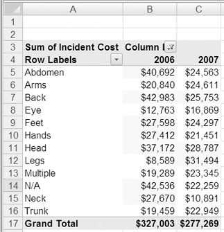
Figure 10-31. Above average cells are highlighted with conditional formatting.

You want to keep the red highlighting for the top three cells, so you'll change the order in which the conditional formatting is applied. If the above average cells are formatted first, then the top three, the red ones, will be visible. To change the order, you'll open the Conditional Formatting Rules Manager dialog box:

1. Select cells B5 to C16, which contain the formatted value cells.
2. On the Ribbon, click the Home tab, and in the Styles group, click Conditional Formatting, and then click Manage Rules.

The Conditional Formatting Rules Manager dialog box opens, where you can see the two rules you created when you applied conditional formatting to the pivot table cells (see Figure 10-32). To the right of the Delete Rule button are the Move Up and Move Down buttons.

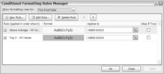
Figure 10-32. Two rules in the Conditional Formatting Rules Manager dialog box

The higher items in the list have precedence over the lower items, and if there is a formatting conflict between rules, the rule with precedence is used. You created the Top 3 rule first, so it is at the bottom of the list. When you created the Above Average rule, it was added to the top of the list, taking precedence over the Top 3 rule. Because the Top 3 cells are also above average, they are affected by both rules, and the formatting for the Above Average rule, which has precedence, is applied last, so the cells are colored yellow.

You'll change the order of the rules so the Top 3 rule has precedence and the red fill color is applied to the Top 3 cells:

1. In the list of rules, click the Top 3 rule.
2. To the right of the Delete Rule button, click the Move Up button to move the Top 3 rule above the Above Average rule.
3. Click OK to close the Conditional Formatting Rules Manager dialog box.

Because you changed the order of the rules, the Top 3 rule now has precedence, and the top three cells are red.

Changing the Pivot Table Layout

Just when you are ready to send the report, the safety director calls to ask whether you can change the report so it shows the injury location per age group per year. You'll add the Age Group field to the report and see whether the conditional formatting needs any changes.

1. Add the Age Group field to the Row Labels area, above the Injury Location field.

   The incident costs change, because they are now broken down by age group. However, the conditional formatting is still applied correctly. The top three amounts are highlighted in red, and all the amounts above average are highlighted in yellow (see Figure 10-33).

   

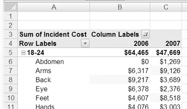
   Figure 10-33. The conditional formatting adjusts to revised layout.

   You're not sure whether the safety director will like the long, narrow report, so you decide to try a different layout.

2. Move the Age Group field to the Column Labels area, below the Year field.

The conditional formatting is now applied to the Year subtotals, and because they are included, the above average cells include all the subtotals and only a few of the other cells (see Figure 10-34).

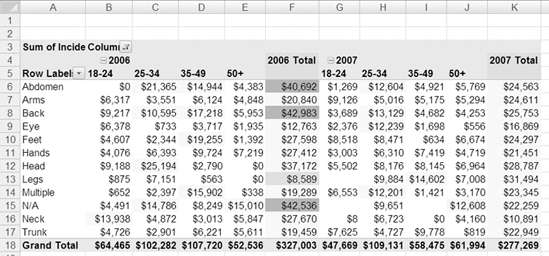
Figure 10-34. The conditional formatting does not adjust correctly.

Instead of having conditional formatting on the entire block of cells, you want the subtotals to be excluded and only the individual values to be formatted. You'll edit the rules to ensure that the subtotals are ignored:

1. Select one of value cells in the pivot table. For example, select cell C8, which is the value for Back in 2006 for the 25–34 age group.
2. On the Ribbon, click the Home tab, and in the Styles group, click Conditional Formatting. Then click Manage Rules.

   The Conditional Formatting Rules Manager dialog box opens, where you can see the two rules that exist for this pivot table. For each rule, the conditional formatting is applied to cells $B$6:$K$17. You'll change this setting in each of the rules, starting with the Above Average rule.

3. In the list of rules, click the Above Average rule.
4. Click the Edit Rule button to open the Edit Formatting Rule dialog box.

   In the Apply Rule To section at the top, there are three options, and the Selected Cells option is currently selected. The range of cells, $B$6:$K$17, is shown (see Figure 10-35).

   

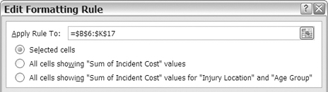
   Figure 10-35. Apply Rule To options in the Edit Formatting Rule dialog box

   The Selected cells option works in many cases, but when you rearrange the pivot table, the conditional formatting may not adjust correctly. In your pivot table, the subtotals are being formatted because they are within the range of cells to which the rule is applied.

   The second option, All Cells Showing "Sum of Incident Cost" Values, would also include too many cells. It would not only include the year subtotals but also the grand totals, because they are also Sum of Incident Cost values.

   The third option, All Cells Showing "Sum of Incident Cost" Values for "Injury Location" and "Age Group," will be the best option for this pivot table. It will restrict the formatting to cells where the Age Group and Injury Location values appear and will exclude the year subtotals and the grand totals.

5. Select the third option, All Cells Showing "Sum of Incident Cost" Values for "Injury Location" and "Age Group."
6. Click OK to close the Edit Formatting Rule dialog box.

   In the Conditional Formatting Rules Manager dialog box, the Above Average rule shows the revised option in the Applies To column. Next, you'll make the same change to the Top 3 rule:

7. In the list of rules, click the Top 3 rule.
8. Click the Edit Rule button to open the Edit Formatting Rule dialog box.
9. In the Apply Rule to section, select the third option, All Cells Showing "Sum of Incident Cost" Values for "Injury Location" and "Age Group."
10. Click OK to close the Edit Formatting Rule dialog box, and click OK to close the Conditional Formatting Rules Manager dialog box.

The conditional formatting is now applied correctly to the individual value cells. The year subtotals and the grand totals are not formatted, and their values are not included in the average calculation. You can send the completed report to the safety director and go for a well-earned lunch break.

Deleting a Rule

When you return to your desk, there's a message from the safety director, who likes the report but thinks it would look better without the Above Average highlighting. You'll delete that rule so only the Top 3 rule will be applied in the pivot table:

1. Select a cell in the pivot table.
2. On the Ribbon, click the Home tab, and in the Styles group, click Conditional Formatting. Then click Manage Rules.
3. In the list of rules, click the Above Average rule.
4. Click the Delete Rule button (see Figure 10-36).
   
   
   

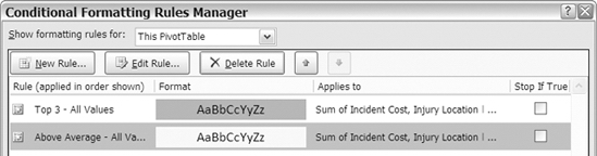
   Figure 10-36. Delete a conditional formatting rule.

5. Click OK to close the Conditional Formatting Rules Manager dialog box.

The Above Average conditional formatting is removed from the pivot table, and only the Top 3 rule formatting remains. You can send the revised report to the safety director and start on the next report on your list.

Setting Format Options

The safety director wants one more report before you leave for the day. Safety meetings will be held in the Illinois and Ohio plants next week, and the safety director wants to take a report that shows the number of Lost Time incidents per month at these locations and the cost of the incidents per year. The pivot table doesn't need any conditional formatting but should be clearly organized and labeled.

You'll clear the existing pivot table and then add the fields you need for the new report.In addition to the standard formatting you have used in other pivot tables, you'll change the pivot table options and some field settings to create an attractive pivot table for distribution at the meetings.

To start, you'll clear the pivot table to remove the current fields and conditional formatting. Then you'll add the fields you need for the new report.

1. Select a cell in the pivot table, and on the Ribbon, under the PivotTable Tools tab, click the Options tab.
2. In the Actions group, click Clear, and then click Clear All to remove all the fields and formatting from the pivot table layout.
3. Add the Plant field to the Row Labels area, and select only Illinois and Ohio from the Row Labels filter list.
4. Add the Year field to the Column Labels area, and add the Month field to the Row Labels area below the Plant field.
5. Add the Report Type field to the Report Filter area, and select Lost Time from the drop-down list.
6. Add the Incident Cost field to the Values area, and add the Date field to the Values area as Count of Date.
7. Format the Incident Cost field as Currency, with zero decimal places.

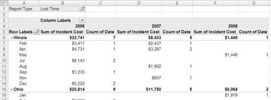
The pivot table data is all in place, and the numbers are formatted correctly, but a few things need improvement (see Figure 10-37). Some of the months are missing for each plant, because no lost time incidents occurred in those months. The pivot table is too wide, because the column headings for the value fields are too long. You also want to clean the pivot table up by hiding some of the features that won't be needed during the meeting, such as the drop-down arrows.

First you'll change the column headings to make them shorter:

1. Click cell B5, which contains the heading Sum of Incident Cost.
2. Type Cost, and then press the Enter key to complete the change.
3. Click cell C5, which contains the heading Count of Date.
4. Type Incidents, and then press the Enter key to complete the change.
   
   
   

   Figure 10-37. The pivot table needs formatting improvements.

Controlling Column Width

All the column headings have changed, and already the pivot table is easier to read and understand. However, when you changed the headings, the columns did not automatically adjust to fit the narrower headings. You'll refresh the pivot table to autofit the columns.

1. Right-click a cell in the pivot table, and in the context menu, click Refresh.

   The pivot table was refreshed, and the columns have adjusted to fit the narrower headings. As you work on this pivot table, you might make adjustments to the columns widths, and you want to prevent further automatic adjustments if the pivot table is refreshed again. You'll change one of the pivot table options to prevent automatic changes to the column widths.

2. Right-click a cell in the pivot table, and in the context menu, click PivotTable Options.
3. In the PivotTable Options dialog box, on the Layout Format tab, remove the check mark from Autofit Column Widths on Update (see Figure 10-38).
   
   
   

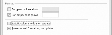
   Figure 10-38. Autofit Column Widths on Update option

4. Click OK to close the PivotTable Options dialog box.

Now, if you manually adjust the column width and then refresh the pivot table, the column width won't change.

Showing Items with No Data

Next, you'll change a setting for the Month field to ensure that all the months are showing for each plant, even if there were no incidents in that month.

1. Right-click a Month label in the pivot table. For example, right-click cell A8, which contains the Apr label for Illinois.
2. In the context menu, click Field Settings.
3. In the Field Settings dialog box, on the Layout Print tab, add a check mark to Show Items with No Data (see Figure 10-39).
   
   
   

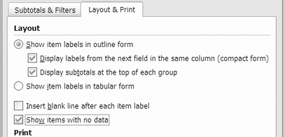
   Figure 10-39. Show Items with No Data option

4. Click OK to close the Field Settings dialog box.

All the months are now listed for each plant, even where there were no incidents in any of the years for that month. This makes it easier to compare the data, since the list of months is consistent between plants.

Hiding Buttons and Labels

As a final step in cleaning up the pivot table, you'll hide the buttons and labels that aren't needed during the meeting. You have applied filters to the Row Labels, and you'll hide that button to prevent any changes during the meeting. You'll also hide the buttons to the left of the Plant labels and you'll remove the Row Labels and Column Labels captions in cells A5 and B3.

1. Right-click a cell in the pivot table, and in the context menu, click PivotTable Options.
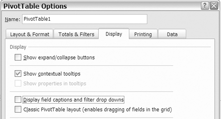
2. On the Display tab, remove the check mark from Show Expand/Collapse Buttons. This will hide the buttons to the left of the plant names.
3. Also remove the check mark from Display Field Captions and Filter Drop Downs (see Figure 10-40). This will hide the filter buttons and the Row Labels and Column Labels captions.
   
   
   

   Figure 10-40. Display options

4. Click OK to close the PivotTable Options dialog box.

The buttons and labels have been removed from the pivot table, giving it a cleaner look. You can make minor adjustments to the column widths so the numbers are well spaced. Because the numbers are right-aligned, you can right-align the column headings, so it's clear which heading is associated with which column of numbers (see Figure 10-41).

The revised pivot table is much improved over the initial version, and you can proudly send it to the safety director for use at the safety meetings in Illinois and Ohio.

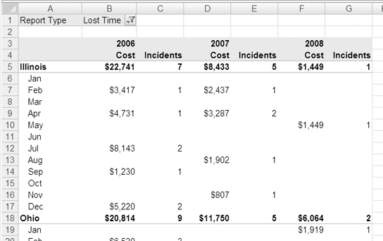
Figure 10-41. Formatted pivot table

Summary

In this chapter, you used conditional formatting to highlight the best and worst results in your safety data. There are many built-in conditional formatting options, and you applied the following types:

• Color Scale
• Icon Set
• Data Bars
• Top 10 Items
• Above Average
• Date Range

In addition to the built-in conditional formatting options, you created custom formats to apply the fill color, font, and other formatting you preferred. You also edited the formatting rules and the order of the rules, so the conditional formatting would work correctly on your pivot table data.

To create a cleaner looking pivot table, you changed the pivot table options to hide buttons and labels when appropriate and to control column width. You also changed the field settings to show items that have no data, such as sales reports where some months have no activity to report.

By using enhanced formatting, you help ensure that your pivot tables are easy to read and understand and that the important information is highlighted in your reports.