
Chapter 5
Magnetic Resonance Technology
5.1 Introduction
Magnetic resonance technology comprises the hardware, software, and imaging techniques used in Magnetic Resonance Imaging (MRI) and Magnetic Resonance Spectroscopy (MRS). MRI has become one of the most useful imaging techniques used in medical diagnosis. Thousands of MRI systems have been produced and installed in clinics since the first introduction to hospitals in the early 1980s. In recognition of the importance of MRI to the practice of medicine, Dr Paul Lauterbur and Sir Peter Mansfield were awarded the 2003 Nobel Prize in Medicine for their discoveries concerning MRI. The Nuclear Magnetic Resonance (NMR) phenomenon, on which MRI is based, was discovered in 1945 by Purcell, Torrey, and Pound at Harvard (1) and independently by Bloch, Hansen, and Packard at Stanford (2). This followed the discovery of electron paramagnetic resonance by J. Zawoysky in 1944. Their work was continued by Hahn (3), who discovered the Spin Echo (SE), and Gabillard (4, 5), who showed that a magnetic field gradient can be used to obtain the spatial distribution of a sample of spins. These discoveries were used exclusively in chemistry until the 1950s, when NMR began to find an application in medicine with the discovery of the relationship between relaxation times and water content in tissue. This was confirmed by Damadian in 1971 (6), who showed that the relaxation times of cancerous and normal tissues may differ. The early 1970s saw the development of diverse MRI approaches by Mansfield (7, 8, 9), Hinshaw (10), Andrew (11), Lauterbur (12), Garroway (13), Hoult (14), Kumar (15), and many others.
MRI allows the visualization of internal structures of a body containing water and fat molecules. Since the human body consists of more than 50% water (about 90% in brain), MRI could be used to image practically any organ. Clinically, MRI is used for early disease diagnosis, while research areas cover new fast imaging techniques, high resolution human and animal anatomy, and details of physiology and pathology. Although the detected signal comes from water or fat molecules, MRI is sensitive to much more than simple Proton Density (PD). The contrast in MR images can come from blood flow, blood oxygenation, water diffusion, or specific properties of tissues, and is called relaxation times. The contrast in an MR image depends on the specific imaging technique used, allowing many types of image appearances, thus giving many options for the clear visualization of specific tissues or physiology. This makes the technique superior in flexibility to other imaging modalities such as Computed Tomography (CT, Chapter 4) or Ultrasound (US, Chapter 11), which use only radiation absorption, reflection, or scattering to obtain an image. Because MR uses only magnetic and radiofrequency (rf) fields, unlike CT, it does not expose the patient to harmful ionizing radiation. MRI can easily provide isotropic 2D or 3D images in any plane, whereas both CT and US techniques are more limited geometrically. Furthermore, MRI suffers from neither heavy absorption in bone (as do X-rays) nor strong reflections from bone (as does US) and thus is ideal for brain and spine imaging—the Central Nervous System (CNS) being encased within bony structures. MRI offers excellent contrast between soft tissues also superior to other modalities.
Owing to this impressive set of advantageous features, the application of MRI has become very broad and includes the diagnosis of many diseases, such as cancer, stroke, brain disorders, and heart conditions. MRI continuously expands into other areas and finds new applications such as the assessment of surgery using intraoperative MRI (16) or image-guided procedures such as biopsy or laparoscopy. The combination of MRI with the specific biochemical information provided by MRS provides potentially a powerful tool for clinical management of problems such as stroke, tumor classification, and monitoring and assessment of other diseases.
To produce an MR image, a strong magnetic field (order of 1 T), time-variable magnetic field gradients, and a rf field are used. As the Signal to Noise Ratio (SNR), and thus image resolution available, increases with the magnetic field strength, as explained in the following sections, there is an industry trend toward the use of stronger magnets. The standard clinical system is equipped with a 1.5-T magnet, but 3-T systems have recently been granted approval by the US Food and Drug Administration (FDA) for clinical use. While stronger magnets (above 3 T) are technically feasible, their possible, yet not proven, harmful side effects and high costs (usually $1M per 1 T for each unit) are the limiting factors. However, new pulse sequences and new types of rf coils are being continuously introduced, improving image quality and extending applications of MRI and MRS.
Many books have been published explaining the principles of MRI (17) and the details of MRI techniques (18, 19).
5.2 Magnetic Nuclei Spin in a Magnetic Field
Atoms with an odd number of nucleons (neutrons + protons) have net non-zero spin, caused by the rotation of charged nuclei. Such spinning nuclei can be imaged with MRI (Table 5.1). Among such atoms are hydrogen (1H), carbon (13C), fluorine (19F), phosphorus (31P), nitrogen (15N), oxygen (17O), and sodium (23Na). These occur in varying abundance within the human body. Owing to the overwhelmingly high content of protons in the tissues (due to water), MRI of hydrogen atoms is predominant in clinical MRI. Some gases, for example, xenon (129Xe) or helium (3H), also possess spin and thus can be imaged after inhalation. However, because of their low density, they must be hyperpolarized (pumped with “extra” energy using laser light) to provide sufficient signal for imaging.
Table 5.1 Properties of Some NMR Sensitive Nuclei
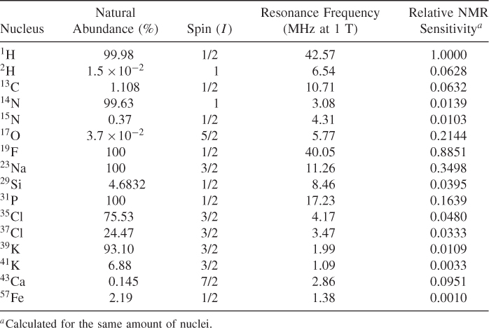
The physics of NMR is described in detail by quantum mechanics, but the classical approach is much easier to understand; therefore, it is herein presented. Following this approach, the spin can be envisioned as a very small rotating magnet, denoted frequently as an arrow (vector). Spins placed in an external magnetic field precess around that field (Fig. 5.1). The frequency of that precession is proportional to the magnetic field and is described by the Larmor equation:
where ω0 is Larmor frequency (in Hz), γ is a gyromagnetic ratio that depends on the nuclei, B0 is the externally applied magnetic field (in tesla). As can be seen from Eq. (5.1), different nuclei precess with different frequencies in the same magnetic field. The frequency of the precession of the most commonly used NMR nuclei and their NMR sensitivities are shown in Table 5.1. Because of the linear relationship between the frequency of rotation and the external field, both ω0 and B0 values are used interchangeably in the literature. For example, one can hear about 1.5 T or 64 MHz MRI system, because 1.5 T corresponds roughly to the proton frequency of 64 MHz (γH = 2.675 rad/sT) and vice versa; 3 T corresponds to 128 MHz. The magnetization created by a nucleus depends also on the type of nuclei because the difference in the energy of the system spins up and down depends on its magnetic moment, which is different for different nuclei. The sensitivity shown in Table 5.1 (last column) shows the signal that could be received from a particular element, assuming the same number of nuclei. The sensitivity of 1H is assumed to be one.
Figure 5.1 Rotation of the spin in the external magnetic field B0.
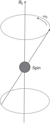
Equation (5.1) describes the behavior of a single spin, whereas in imaged objects there are many spins (order of 1024). When such an object is placed in a magnetic field, its spins align either parallel or anti-parallel to the field (Fig. 5.2). There is only a very small difference, about one per million, between the number of spins aligned parallel to the field and those aligned antiparallel. This small difference makes MR less sensitive than other imaging methods, such as infrared spectroscopy (Chapter 9). This excess of spins creates a net magnetization, which is detected by MR systems as the NMR signal. The amplitude of the magnetization depends on the strength of the external magnetic field. For instance, in the Earth's magnetic field the magnetization is practically undetectable. Therefore, very strong magnetic fields must be generated by specially designed magnets (most frequently superconductive) to be able to produce enough signal. The magnetic fields used in present clinical MRI systems vary from 0.2 to 3 T (the Earth's magnetic field is about 50 μT, i.e., about 500,000 times lower). Experimental MRI systems currently reach 14 T, while systems for NMR spectroscopy approach 20 T (almost 1 GHz for protons).
Figure 5.2 Spins placed in the external magnetic field B0 create net magnetization ![]() along the direction of the field.
along the direction of the field.
5.2.1 A Pulsed rf Field Resonates with Magnetized Nuclei
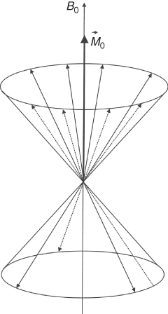
As explained above, there is a net magnetization created when magnetic nuclei are placed in a magnetic field. In other words, the patient becomes magnetized. The application of an external rf field (or precisely its magnetic component B1) in the plane perpendicular to the external magnetic field, crucially at the rf corresponding to the frequency of the rotating spins, “flips” some or all of them from up to down position (Fig. 5.3). This phenomenon is known as nuclear magnetic resonance (NMR).
Figure 5.3 (a) Spin rotates around the magnetic field B0. (b) Application of the rf pulse, corresponding to the frequency of the spin rotation, flips the spin.
To understand what happens after the rf pulse is applied, let us assume that the external magnetic field is applied in the z direction and the rf pulse is applied in x-y plane. Before the pulse is applied, ![]() (the sum vector of all spins) is in equilibrium and is aligned along the external
(the sum vector of all spins) is in equilibrium and is aligned along the external ![]() magnetic field (Fig. 5.3a). Following the application of the rf pulse, the net magnetization
magnetic field (Fig. 5.3a). Following the application of the rf pulse, the net magnetization ![]() flips away from its equilibrium position (Fig. 5.4). This tilt is called the flip angle (φ) and depends on the product of the amplitude and duration of the rf pulse. For a rectangular pulse of duration tp, and rf amplitude B1, the flip angle can be expressed as φ = γB1tp or more generally for a pulse of any shape:
flips away from its equilibrium position (Fig. 5.4). This tilt is called the flip angle (φ) and depends on the product of the amplitude and duration of the rf pulse. For a rectangular pulse of duration tp, and rf amplitude B1, the flip angle can be expressed as φ = γB1tp or more generally for a pulse of any shape:
where B1(t) is the envelope of the rf pulse of duration tp.
Figure 5.4 (a) Application of the φ degree rf pulse tilts the magnetization ![]() from its equilibrium position along the z direction by the angle φ. (b) Magnetization lies along the x direction after the 90° rf pulse is applied.
from its equilibrium position along the z direction by the angle φ. (b) Magnetization lies along the x direction after the 90° rf pulse is applied.
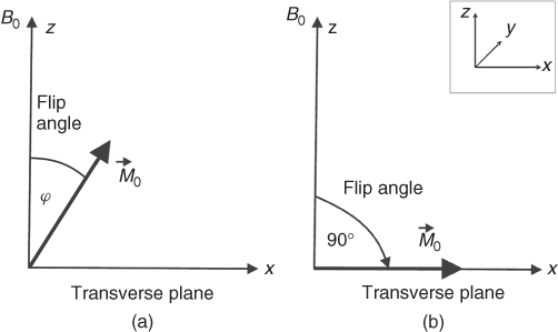
As can be seen from Eq. (5.2), the stronger the rf field applied or the longer it lasts the larger the flip angle. An rf pulse that flips the magnetization 90° from the equilibrium position is termed 90° (or π/2) pulse, and similarly for other flip angles (45°, 180°, etc.). The maximum NMR signal available from a sample is obtained after a 90° pulse.
5.2.2 The MR Signal
To produce the rf field and detect the signal, rf coils (often referred to as rf probes or resonators or incorrectly as antennas) are used. The simplest rf coil is a solenoid. The coils are designed to produce their rf field in x-y plane (Fig. 5.5). After the application of a 90° rf pulse, the magnetization ![]() rotates along the z direction in the x-y plane. The Mxy component of the magnetization induces a voltage in the coil that can be amplified and detected. The rf pulse not only flips the spins but also imposes the phase coherence of the spins. Immediately after, the rf pulse (Fig. 5.6b) spins have the same phase, but soon after they dephase because each spin rotates in a slightly different magnetic field due to inhomogeneities of the magnetic field (order of 10−6 of the main field in standard MRI magnets). Inhomogeneous magnetic field means that there is a different field at each point. Thus, spins within the same field rotate with slightly different frequencies that depend on their position
rotates along the z direction in the x-y plane. The Mxy component of the magnetization induces a voltage in the coil that can be amplified and detected. The rf pulse not only flips the spins but also imposes the phase coherence of the spins. Immediately after, the rf pulse (Fig. 5.6b) spins have the same phase, but soon after they dephase because each spin rotates in a slightly different magnetic field due to inhomogeneities of the magnetic field (order of 10−6 of the main field in standard MRI magnets). Inhomogeneous magnetic field means that there is a different field at each point. Thus, spins within the same field rotate with slightly different frequencies that depend on their position ![]() , causing an overall spin vector dephasing. As spins lose their phase coherence, the amplitude of the induced MR signal decreases. This natural process is known as Free Induction Decay (FID), and its exponential decrease is described by time called
, causing an overall spin vector dephasing. As spins lose their phase coherence, the amplitude of the induced MR signal decreases. This natural process is known as Free Induction Decay (FID), and its exponential decrease is described by time called ![]() (“t 2 star”).
(“t 2 star”).
Figure 5.5 Rotating magnetization ![]() induces current in the receiving rf coil.
induces current in the receiving rf coil.
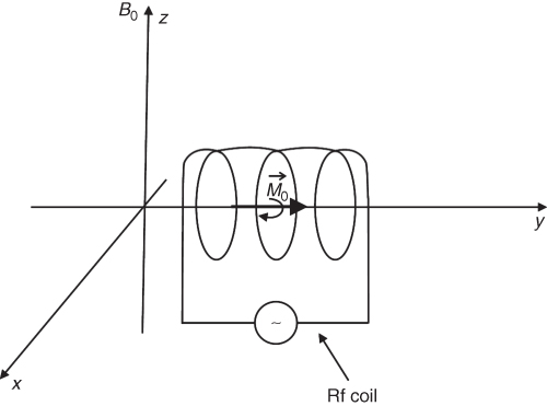
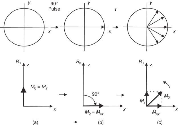
Figure 5.6 Behavior of the magnetization ![]() in the external magnetic field B0 along the z direction: x-y plane (top row), z-x plane (bottom row): (a) Magnetization in equilibrium; (b) magnetization just after 90° rf pulse; (c) magnetization returns to equilibrium after time t from the application of the 90° rf pulse; spins dephase in x-y plane.
in the external magnetic field B0 along the z direction: x-y plane (top row), z-x plane (bottom row): (a) Magnetization in equilibrium; (b) magnetization just after 90° rf pulse; (c) magnetization returns to equilibrium after time t from the application of the 90° rf pulse; spins dephase in x-y plane.
5.2.3 Spin Interactions have Characteristic Relaxation Times
As mentioned above, the signal induced in the rf coil (caused by Mxy) decreases with time because of the inhomogeneity of the external magnetic field. This is, however, not the only reason that causes the signal to decay. Before the 90° pulse is applied, there is a net magnetization along the z direction (![]() ) (Fig. 5.6a). The 90° rf pulse flips magnetization
) (Fig. 5.6a). The 90° rf pulse flips magnetization ![]() to the x-y plane, creating a net magnetization in the x-y plane (Mxy) (Fig. 5.6b). At that point, the Mz component is zero. After the rf pulse is removed, the net magnetization Mz returns, like all natural processes, to equilibrium (Fig. 5.6c); this process of rebuilding Mz is called longitudinal or spin-lattice relaxation. The time constant describing the recovery of the magnetization is known as the T1 relaxation time. The decay of the magnetization Mxy in the x-y plane is called transverse or spin-spin relaxation or T2 decay. One can show that (for a Lorentzian spectral function)
to the x-y plane, creating a net magnetization in the x-y plane (Mxy) (Fig. 5.6b). At that point, the Mz component is zero. After the rf pulse is removed, the net magnetization Mz returns, like all natural processes, to equilibrium (Fig. 5.6c); this process of rebuilding Mz is called longitudinal or spin-lattice relaxation. The time constant describing the recovery of the magnetization is known as the T1 relaxation time. The decay of the magnetization Mxy in the x-y plane is called transverse or spin-spin relaxation or T2 decay. One can show that (for a Lorentzian spectral function) ![]() thus
thus ![]() and T2 are defined exactly as the time needed for 63% of the Mz to recover and Mxy to decay, respectively. The details of the processes causing the relaxation can be found, for example, in Reference (20). Generally, the longitudinal relaxation is caused by the rotational and translational molecular motion, which creates a small time-varying magnetic field as seen by the spin, and which causes spins to flip and transfer their energy to the surrounding molecules (lattice). Therefore, this type of relaxation is particularly efficient in the presence of paramagnetic substances (such as O2). Thus, pure, degasified water has a T1 of about 4 s (the exact value depending on the external magnetic field and temperature), whereas water in brain or blood has a T1 of about 100 ms because of dissolved ions creating fluctuating magnetic fields. As a result, the energy of the spins dissipates as heat (although a very small amount). Conversely, the transverse relaxation (T2) is caused by interactions among spins themselves. Each flip of a spin changes the local magnetic field, which in turn affects surrounding spins and accelerates the transition of spin from one position to the other. Contrary to longitudinal relaxation, there is no net heat created in this process. As in all natural processes, the relaxations have exponential behavior and can be mathematically described, following the 90° pulse, as
and T2 are defined exactly as the time needed for 63% of the Mz to recover and Mxy to decay, respectively. The details of the processes causing the relaxation can be found, for example, in Reference (20). Generally, the longitudinal relaxation is caused by the rotational and translational molecular motion, which creates a small time-varying magnetic field as seen by the spin, and which causes spins to flip and transfer their energy to the surrounding molecules (lattice). Therefore, this type of relaxation is particularly efficient in the presence of paramagnetic substances (such as O2). Thus, pure, degasified water has a T1 of about 4 s (the exact value depending on the external magnetic field and temperature), whereas water in brain or blood has a T1 of about 100 ms because of dissolved ions creating fluctuating magnetic fields. As a result, the energy of the spins dissipates as heat (although a very small amount). Conversely, the transverse relaxation (T2) is caused by interactions among spins themselves. Each flip of a spin changes the local magnetic field, which in turn affects surrounding spins and accelerates the transition of spin from one position to the other. Contrary to longitudinal relaxation, there is no net heat created in this process. As in all natural processes, the relaxations have exponential behavior and can be mathematically described, following the 90° pulse, as ![]() . Both processes, the return of Mz to its equilibrium and the decay of Mxy to zero, can be probed by an MR system and exploited to obtain image contrast.
. Both processes, the return of Mz to its equilibrium and the decay of Mxy to zero, can be probed by an MR system and exploited to obtain image contrast.
5.3 Image Creation
To create an MR image, the main magnetic field, three gradients of the magnetic field, and an rf field are all required. This section describes mathematically how an image can be created if all these requirements are provided.
5.3.1 Slice Selection
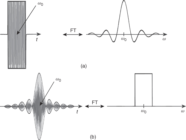
One of the advantages of MRI over other imaging techniques is the possibility of selection of the slice of interest. To understand how the slice is selected, we will first consider the rf pulses used in MRI. As mentioned before, rf pulses are needed to generate an MR signal. There are two types of rf pulses: non-selective and selective (Fig. 5.7). Each pulse used in MRI is “filled” with an rf field corresponding to the Larmor frequency. Therefore, its shape is called an envelope function. A detailed analysis of the rf pulses, for example (21), reveals that each pulse has its own frequency spectra. It means that an rf pulse “contains” not only one particular frequency but rather a band of frequencies, the distribution of which depends on the shape (envelope function) of the rf pulse. For example, a very long (infinite) sinusoidal pulse in the time domain (s(t) = sinω0t) produces only one frequency (ω0) in the frequency domain, but a rectangular pulse has a spectrum of frequency distributed around the central frequency ω0 and decreasing with the frequency offset from ω0 (Fig. 5.7a). The most commonly used selective pulses in MRI are pulses with so-called sinc (sinc(x) = sinx/x) envelope (Fig. 7b), because their frequency spectra is nearly rectangular, leading to a rectangular slice profile. Other complex pulses, for example, based on Hermite function, are also used, as their slice profile is even closer to rectangular than the sinc function.
Figure 5.7 (a) Selective (soft) rf pulse and its Fourier transform. (b) Nonselective (hard) rf pulse and its Fourier transform.
The mathematical formula describing the relationship between the time and frequency domains is called a Fourier Transform (FT): ![]() , where F(ω) is the frequency domain of the signal S(t) in the time domain (22). Interestingly, the inverse FT links F(ω) with
, where F(ω) is the frequency domain of the signal S(t) in the time domain (22). Interestingly, the inverse FT links F(ω) with ![]() . The FT is of fundamental importance in MRI, where it is used to process the MR signal to obtain an MR image. FT was first applied in NMR by Richard Ernst in 1966 (23). The application of FT to NMR later allowed the extension to MRI and the subsequent development of other imaging techniques. The simultaneous application of the constant gradient (
. The FT is of fundamental importance in MRI, where it is used to process the MR signal to obtain an MR image. FT was first applied in NMR by Richard Ernst in 1966 (23). The application of FT to NMR later allowed the extension to MRI and the subsequent development of other imaging techniques. The simultaneous application of the constant gradient (![]() ) of the magnetic field and the selective rf pulse allows slice selection (Fig. 5.8). When the gradient is applied, for example, along the z direction (
) of the magnetic field and the selective rf pulse allows slice selection (Fig. 5.8). When the gradient is applied, for example, along the z direction (![]() ), the frequency of the spins (Eq. 5.1) depends on their position along that direction (
), the frequency of the spins (Eq. 5.1) depends on their position along that direction (![]() ). The stronger the gradient and/or the narrower the rf pulse bandwidth (BW) the thinner the selected slice, according to the formula: Δz = Δω/γGz, where Gz is a constant gradient in the z direction, Δω is the BW of the rf pulse, and Δz is the slice thickness. In modern MRI systems, gradient coils can generate field gradients up to 40 mT/m, which along with the application of a standard selective rf pulse of several kHz BW allows submillimeter slice thicknesses.
). The stronger the gradient and/or the narrower the rf pulse bandwidth (BW) the thinner the selected slice, according to the formula: Δz = Δω/γGz, where Gz is a constant gradient in the z direction, Δω is the BW of the rf pulse, and Δz is the slice thickness. In modern MRI systems, gradient coils can generate field gradients up to 40 mT/m, which along with the application of a standard selective rf pulse of several kHz BW allows submillimeter slice thicknesses.
Figure 5.8 Process of slice selection using gradient of the magnetic field and selective rf pulse. (a) Selective rf pulse corresponding to the frequency 63.98 ± 0.01 MHz selects a slice of Δz thickness. (b) The same rf pulse as in (a), but the gradient is two times stronger: slice thickness is now half as wide as above.
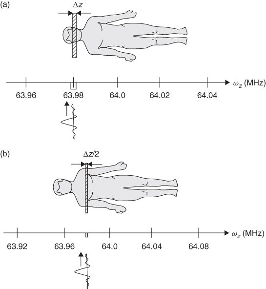
To analyze in detail the slice selection process shown in Figure 5.8, let us assume that a patient is lying in the 1.5-T magnet and both the main field and the gradients are applied along the z direction. And let us also assume that the frequency in the center of the magnet is exactly 64.00 MHz. If we add a magnetic field gradient to the main field, the precession frequency of the spins in a patient's body will depend on their position: spins will precess faster in the legs and slower in the head. If we now apply a selective rf pulse, with the spectrum width ![]() MHz and with frequency ω0 corresponding to the frequency of the spins rotating in the head (63.98 MHz) (Fig. 8a) we excite, thus select, only spins in the slice Δz that spins rotate at the frequency 63.98 ± 0.01 MHz. What happens is that the band of frequencies presents in the rf pulse matches the resonant frequencies of the spins within a thin slice of the patient.
MHz and with frequency ω0 corresponding to the frequency of the spins rotating in the head (63.98 MHz) (Fig. 8a) we excite, thus select, only spins in the slice Δz that spins rotate at the frequency 63.98 ± 0.01 MHz. What happens is that the band of frequencies presents in the rf pulse matches the resonant frequencies of the spins within a thin slice of the patient.
In a second experiment, we use the same selective rf pulse but double the strength of the gradient (Fig. 5.8b) and thus select a different slice (e.g., through a chest), because now the spins rotating with the frequency matching that of the rf pulse are “shifted” (to the right in Fig. 5.8b) because of the stronger gradient. Furthermore, the selected slice Δznew in now only half as wide, because now the same Δω corresponds to half the thickness of the previous slice: Δznew = Δω/γ2Gz. In other words, we have narrowed the frequency window. In this way, slice thickness could be controlled.
The other way of changing the slice thickness is to use a selective pulse with a narrower spectrum. This could be accomplished, for example, by using longer, thus more selective rf pulses or by changing their shape. To select a different slice but of the same thickness, an rf pulse with different center rf frequency is used. Unfortunately, selective pulses do not have perfect rectangular spectra; therefore, spins may experience slightly different rf fields across the slice and their flip angles may be different. Such “slice profile” effects can be the source of artifacts.
5.3.2 The Signal Comes Back—The Spin Echo
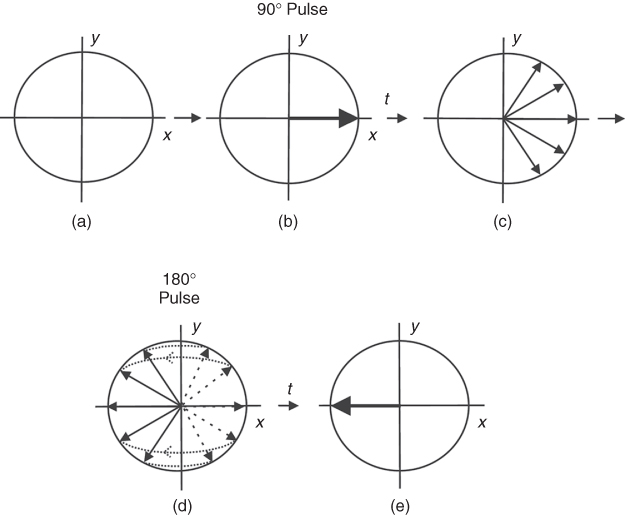
To understand how an MR image is created, first we will explain the spin (or Hahn) echo. The SE was discovered by Erwin Hahn in 1950 (3). As we already know, the application of a 90° rf pulse with frequency corresponding to the frequency of the rotating spins creates a net magnetization in x-y plane (Fig. 5.9). Owing to the inhomogeneities of the magnetic field and the relaxation T2, the spins dephase after the rf pulse is removed, leading to decay of the MR signal. This process is detected by the rf receiver coil as the FID with the T2* time. Because FID occurs just after the rf pulse and is usually very short, its detection is rather difficult. Therefore, often additional rf pulses are used to collect the MR data. The most common is the application of the 180° pulse after the 90° pulse. The 180° pulse, also called a refocusing pulse, flips all spins vectors by 180° about some axis. Specifically, a ![]() pulse (180° with y phase) flips the spins about the y axis. (The
pulse (180° with y phase) flips the spins about the y axis. (The ![]() pulse would flip the spins along x axis.) As can be seen from Figure 5.9, the spins dephasing will now rephase again, and exactly after the same time (t) as 180° pulse was applied after 90° pulse, they will all align along the y axis. In other words, after the 180° pulse is applied, the spins that rotated fast (dephased faster) will continue to rotate faster, but now they will chase the slower rotating spins to catch them up on the y axis, exactly after the same time as the time interval between 90° and 180° pulses. To explain the SE phenomenon, many authors bring an analogy of the sprinters beginning the race at the same start point and then, at any point during the race, they suddenly (180° pulse) move back with the same speed (as in a move played backwards). As one can easily imagine, all sprinters will reach the starting point at the same time (they will be in phase again). Fortunately, in real life, the time cannot be set backwards, so there is a sense of running fast if you want to win!
pulse would flip the spins along x axis.) As can be seen from Figure 5.9, the spins dephasing will now rephase again, and exactly after the same time (t) as 180° pulse was applied after 90° pulse, they will all align along the y axis. In other words, after the 180° pulse is applied, the spins that rotated fast (dephased faster) will continue to rotate faster, but now they will chase the slower rotating spins to catch them up on the y axis, exactly after the same time as the time interval between 90° and 180° pulses. To explain the SE phenomenon, many authors bring an analogy of the sprinters beginning the race at the same start point and then, at any point during the race, they suddenly (180° pulse) move back with the same speed (as in a move played backwards). As one can easily imagine, all sprinters will reach the starting point at the same time (they will be in phase again). Fortunately, in real life, the time cannot be set backwards, so there is a sense of running fast if you want to win!
Figure 5.9 Spin echo: (a) magnetization in equilibrium; (b) 90° rf pulse applied; (c) spins dephasing for time t; (d) 180° rf pulse applied, spins rephasing; and (e) spins align along the y axis as in (b) after time t.
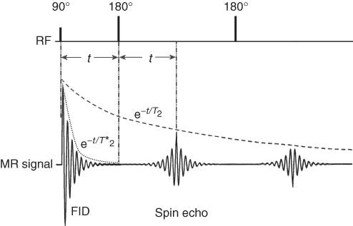
The application of a series of 180° pulses following the 90° pulse creates a series of SEs (Fig. 5.10), as each 180° keeps refocusing spins. If there were no relaxation processes, as assumed above, the amplitude of each echo would remain constant. However, in reality, between the application of a 90° pulse and the detection of each SE, spins interact with each other (T2 relaxation), causing some of them “to be lost” in this time, thus reducing the amplitude of the echoes. Therefore, echo train amplitude will be decreasing with T2 constant. The application of a ![]() pulse followed by a series of
pulse followed by a series of ![]() pulses is called the CPMG pulse sequence, from the name of its discoverers in 1954: Carr, Purcell, Meiboom, and Gill (24). This is the most frequently used method of measurement of the T2 relaxation time in MR.
pulses is called the CPMG pulse sequence, from the name of its discoverers in 1954: Carr, Purcell, Meiboom, and Gill (24). This is the most frequently used method of measurement of the T2 relaxation time in MR.
Figure 5.10 MR signal created by a 90° pulse and a series of 180° pulses (CPMG pulse sequence). The FID of the signal following the 90° pulse depends on T2*; the curve connecting peaks of echoes created by series of 180° pulses is T2 dependent.
5.3.3 Gradient Echo
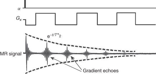
The other method of obtaining an MR signal in the form of an echo is the so-called Gradient Echo (GE). This method allows a much faster acquisition of the signal because it does not require the application of 180° rf pulses. Instead of the refocusing rf pulses, typically lasting about 2–5 ms, a gradient reversal is used (Fig. 5.11). Following the low angle rf pulse (usually 5–15°) for the fast data acquisition, a negative gradient is applied, followed by the reverse gradient of the same duration and amplitude. The negative gradient causes the spins to rotate with different frequencies that depends on the spins' spatial position (ω = γGxx), causing their dephasing with time. Following the negative gradient, the positive one is applied, causing spins to refocus, as now the faster defocusing ones are faster to refocus. However, unlike SE, GE is affected by the main field inhomogeneities, because this effect is not cancelled by the rf refocusing pulses. The rf refocusing 180° pulse, in contrary to the switching gradients, reverses the effects of the inhomogeneous field. As a consequence, the GEs are T2* dependent. The switching gradients, as refocusing pulses, can be repeated to obtain a GE train (Fig. 5.11) and used in GE imaging (Section 5.8).
Figure 5.11 Gradient echoes created by a switching gradient. The decay curve is T2* dependent.
Advanced readers may be interested in the so-called stimulated echo, which is created by three rf pulses. Because of the need for three rf pulses and an amplitude of only half that of an SE, the stimulated echo is not commonly used in MRI (3). In addition, stimulated echoes may present as image artifacts in sequences using more than two rf pulses for the single excitation. However, the stimulated echo has found an application in localized MR spectroscopy.
5.4 Image Reconstruction
Now that basic MR terminology and phenomena have been covered, we can proceed with the details of the nature of the MR image creation.
To understand how an MR image is created, we shall consider a pulse sequence based on SE, as shown in Figure 5.12. The general principles of other pulse sequences are similar. Section 5.3.1 discussed how a slice is selected using simultaneously the selective rf pulse and the gradient of the magnetic field. As shown in Figure 5.12a gradient in the z direction and a selective rf pulse are used to excite spins in the desired slice. The application of two additional orthogonal gradients in x and y directions allows information about the spatial position of the spins.
Figure 5.12 Slice-selective spin echo (SE) pulse sequence: Gz, slice selection gradient; Gy, phase encoding gradient; Gx, frequency encoding gradient, TR, repetition time, and TE, echo time.
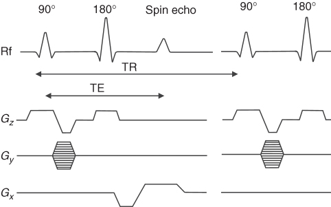
The y gradient (Gy) applied after the first rf pulse for a short time t causes the spins to rotate with a different frequency along y, thus accumulating a final phase (φ(y) = γGyyt) that depends on the position of the spins along the y direction (Fig. 5.13). This gradient is called phase encoding. (The gradient with the same amplitude and duration is also applied after SE sequence to begin the next acquisition from the same spin settings; this is omitted in Fig. 5.12 for simplicity.)
Figure 5.13 (a) Spins of the object placed in the perfectly homogenous magnetic field. (b) Spins change phase and frequency after the application of two perpendicular gradients.
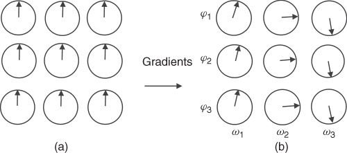
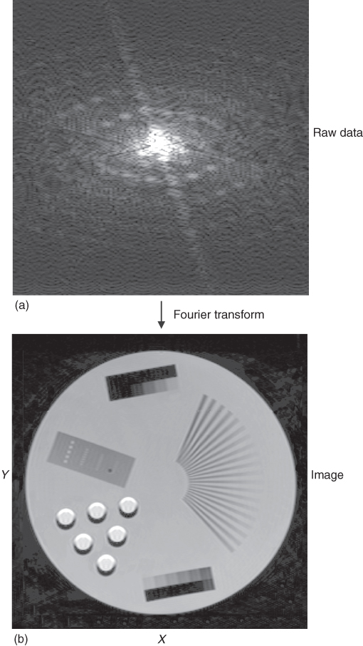
The application of the second gradient along the x direction (the so-called read gradient) during the acquisition of the SE causes spins to rotate with a frequency dependent on the x position of the spins. This way, each spin has a different frequency or phase depending on its spatial position. The electronics used in MR can detect the phase and frequency of the MR signal. The pulse sequence has to be repeated with different amplitudes of the phase encoding gradient to reconstruct an image in two dimensions, as the multiple phases in a single data acquisition cannot be resolved. The acquired data (SE) is digitized using an Analog to Digital Converter (ADC) and stored in the computer memory, and then the 2-dimensional (2D) FT converts frequency into position, first along read direction and then along the phase direction to reconstruct a 2D image. The details of the FT procedure can be found, for example, in Reference 19. The time interval between data points collected along the read direction is called sampling rate, which is the inverse of the receiver sampling BW. The raw data collected by an MRI system and an image created after FT is applied are shown in Figure 5.14. The top picture shows the data (sampled echo) collected with different phase encoding gradients starting from its positive maximum value (first row) down to maximum negative value (last row). The maximum MR signal, and the most valuable information about an imaged object, is collected in the center of the data matrix (center line), where phase encoding gradient is close to zero. The raw data is often referred to as k-space. An introduction of the k-space concept simplified the mathematical description of MRI methods; however, its analysis is beyond the scope of this chapter, but can be found, for example, in References 19, 21.
Figure 5.14 (a) The raw data acquired by the MRI system. Each horizontal line corresponds to echo obtained at different phase gradients. The read gradient is constant for each line. (b) Image obtained after 2D FT is applied to the raw data.
The described method applies to all MRI techniques, as one direction is always frequency encoding and the other phase encoding, and 2D FT is used for image reconstruction.
As mentioned earlier, phase encoding must be repeated to be able to obtain 2-dimensional information about the object. Therefore, the spins must be excited more times, thus the rf pulses, 90° and 180°, as well as all the gradients are applied repetitively, but each time the amplitude of the phase encoding gradient varies.
5.4.1 Sequence Parameters
The time between each consecutive 90° rf pulse is called Repetition Time (TR), while the time between a 90° pulse and the maximum amplitude of the echo is called Echo Time (TE) (Fig. 5.12). The time required to obtain data to create an image is called the total acquisition time (or scan time). For pulse sequences that require multiple excitations, the total acquisition time is equal to TR multiplied by number of phase encoding steps. To increase SNR and image quality, the pulse sequence may be repeated and data co-added, but at the expense of an extended total acquisition time.
Proper selection of such sequence parameters allows different MR image contrast to be obtained. This selectable image contrast is a major difference between MRI and other imaging techniques. This unique feature dramatically enhances diagnostic capabilities of MRI, as tissue contrast can be tailored to the disease under investigation. This also makes MRI interpretation more complex because a tissue, for example, fat or blood, may be bright on one image but dark on another, depending on a pulse sequence and parameters used.
5.5 Image Resolution
As explained in Section 5.3.1, the imaged slice in MRI is selected by the gradients and the selective rf pulse. In medical practice, the most commonly used slice thickness, an important MR image parameter, is around 1 mm. While a thinner slice would ideally provide more precise diagnostic information, thinner slices also require longer scan times to produce image with high enough quality. An equally important MR image parameter is in-plane or spatial resolution. Spatial resolution is defined as the separation between two neighboring points of the imaged object, which can be distinguished. In MRI, spatial resolution depends on the Field of View (FOV) and the number of points (pixels) along each direction (Chapter 2). The number of pixels in the read direction depends on the number of collected (sampled) data points. The number of phase encoding gradient steps used to collect each row of data determines the image resolution in the phase encoding direction. However the raw data matrix may be different from the image matrix because of postprocessing methods such as zero filling (increasing the size of the data matrix by filling the data with zeros before FT), which are used to improve displayed image quality (while remaining the same scan time).
The image resolution depends on the size of the imaged object and the matrix size. For example, for human head imaging, FOV is usually 24 cm and data matrix 256 × 256. These parameters give in-plane resolution of 0.94 mm × 0.94 mm (FOV/matrix size = 0.94 mm). For a smaller object, say a finger, FOV may be 2 cm and matrix, 256 × 256, which gives an in-plane resolution of 78 μm × 78 μm.
The question arises: what are the limits of resolution? Couldn't we just increase the number of sampling points and phase encoding steps to increase the resolution indefinitely? Unfortunately, there is no simple answer, as there are important trade-offs that limit the resolution: signal-to-noise ratio (SNR), gradients strength, rf power, and diffusion. The limits of gradient strength and rf power are due to hardware limitations and subject safety (see Section 14), diffusion is a property of a living tissue, while SNR limit as associated with both physics and hardware.
The FOV and hence the image resolution limit due to the gradients strength is described by Nyquist theorem:
5.3 ![]()
where Δt is the sampling rate in the read direction or the duration of the phase gradient and G is the amplitude of the gradient. As can be seen from the equation, the FOV is inversely proportional to the gradient strength. The amplitude of the gradients is limited by the construction of the gradient coils, by the gradient amplifiers, and ultimately by safety concerns. Currently, gradient amplifiers producing 2 kV and a few hundred amperes are used to generate a 40-mT/m gradient in clinical systems, while smaller experimental MRI systems can provide a gradient stronger than 1000 mT/m, allowing resolution of about 10 μm. An additional safety issue in human systems is the regulatory limits on gradient rise time (dB/dt) imposed to avoid nerve stimulation.
Water molecules in biological objects move with the speed of about 2 μm/ms due to diffusion. This process is yet another limitation of the resolution in MRI, and in particular in MR microimaging, where resolution reaches 10 μm or even less. Diffusive motion in the presence of the strong and long gradient required for high resolution leads to signal loss from irreversible dephasing.
5.6 Noise in the Image—SNR
There are a few different definitions of SNR. In MRI, SNR is usually defined as the ratio of the averaged signal intensity over the imaged object (or part of it) to the average noise intensity, calculated over a small area outside the imaged object (i.e., noise background). It can also be defined as the ratio of the mean signal intensity within the imaged object to the standard deviation of the background noise selected outside the object. Both definitions describe how strong the signal is in relation to the noise. In MRS, SNR is usually defined as the ratio of the signal amplitude to the average baseline noise. Of course, the higher the SNR the better image quality, which in turn can allow higher resolution. Without high SNR, high resolution images, although technically feasible, cannot provide meaningful images. Frequently the term Contrast-to-Noise Ratio (CNR) is also used to describe image quality and its value in detecting pathology. CNR is a measure of the difference in contrast between two tissues, relative to overall SNR. CNR can be improved by the selection of proper parameters of the pulse sequence, to best emphasis the difference in relaxation times, as described in Section 5.7.
Quantum mechanics shows that the MR signal is proportional to the square of the strength of the main magnetic field (![]() ) and to the number of spins, namely, the volume of the sample (20). The undesired noise comes from the random thermal motion of water (and other) molecules of the sample and electronic noise of the MR system, including the noise of the receiver coil and the preamplifier. Therefore, SNR depends on many factors such as the strength of the magnetic field, resistance and quality factor (Q) of the coil, its geometry, sample volume, filling factor of the coil, and so on.
) and to the number of spins, namely, the volume of the sample (20). The undesired noise comes from the random thermal motion of water (and other) molecules of the sample and electronic noise of the MR system, including the noise of the receiver coil and the preamplifier. Therefore, SNR depends on many factors such as the strength of the magnetic field, resistance and quality factor (Q) of the coil, its geometry, sample volume, filling factor of the coil, and so on.
Experience has lead to a rule of thumb that says that, if all other aspects of the experiment are held constant, SNR is proportional to the main magnetic field strength. This formula holds for human systems up to 3 T. The detail analysis of SNR was first presented by Hoult (25). A relatively easy way of improving SNR is multiple acquisitions of the same data. This is accomplished by repeating the pulse sequence with identical parameters and adding the collected data. This is called repetition, or averaging (N), or number of excitations (Nex). It may be proved that SNR increases with the root square of the repetitions (![]() ). Because each repetition increases the total scan time twofold to double SNR requires a fourfold longer acquisition time, so this approach clearly has its practical limits. The linear relationship between the field strength and the SNR explains the tendency to introduce stronger magnets as an effective, yet expensive, way of increasing SNR.
). Because each repetition increases the total scan time twofold to double SNR requires a fourfold longer acquisition time, so this approach clearly has its practical limits. The linear relationship between the field strength and the SNR explains the tendency to introduce stronger magnets as an effective, yet expensive, way of increasing SNR.
5.7 Image Weighting and Pulse Sequence Parameters TE and TR
The signal induced by the magnetization in an rf coil is proportional to the number of excited protons in the imaged object, thus regions with higher PD exhibit a stronger signal. These signal differences can be observed using PD-weighted (PD or ρ) MRI; however in general, the variation in PD between healthy and diseased tissue is rather small. Fortunately for MRI's clinical diagnostic applications, there are better alternatives.
Abnormal tissues vary in a number of parameters including T1, T2 and T2* relaxation times, also diffusion, blood flow, susceptibility, and various other effects that influence the MR signal in detectable ways.
While MRI does allow the precise quantification of these parameters, it is more common to use the “weighted” MR techniques. As an example, T1-weighted imaging means that the image contrast is created mostly (although not entirely) based on the differences in T1 values of the tissues. A similar terminology applies to T2, PD, or Diffusion-Weighted (DW) MRI. In this way, tissues with generally rather similar proton densities but differing in some other tissue property can be better visualized (Fig. 5.15). For instance, cancerous tissues can be better identified using T1 or T2 than PD. So how is this achieved in practice?
Figure 5.15 MR images of the brain. (a) T1 weighted (GE pulse sequence: TR = 475 ms, TE = 2.46 ms; slice thickness 4 mm, FOV = 25 cm). (b) PD weighted (SE pulse sequence: TR = 3000 ms, TE = 20 ms, slice thickness 4 mm, FOV = 22 cm). (c) T2 weighted (SE pulse sequence: TR = 6000 ms, TE = 90 ms, FOV = 22 cm; slice thickness 4 mm).

5.7.1 T2-Weighted Imaging
As explained in Section 5.2.3, the decay of the echo amplitudes in an SE pulse sequence depends on the T2 relaxation time. Therefore, the longer the TE the lower the amplitude of the echo due to T2 relaxation. For example, consider two tissues (Fig. 5.16): A with short T2 (for example, fat or muscle tissue) and B with long T2 (e.g., cyst or blood). If we chose a very short TE, little T2 weighting will develop, and the difference in the amplitudes of echoes from both tissues will be small. However, if we use a longer TE (typically of the order of T2 or longer), the difference in the echo amplitudes increase and become detectable. To totally avoid any T1 contribution, TR must be rather long (5T1 or longer).
Figure 5.16 Return of magnetization after a 90° pulse in the y direction for tissues with (a) short T2 and (b) long T2.
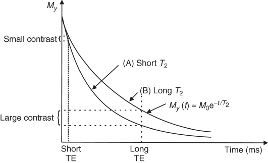
Because relaxation times depend on both the imaged tissue and the main magnetic field strength, the optimal TE and TR values parameters vary. However, the standard parameters for clinical T2-weighted MRI are TE > 80 ms and TR > 2000 ms. A longer TR increases total scan time; therefore, often T2-weighted images have some contribution of T1. To avoid T1 weighting, TR should be longer than 5 s, as T1 of tissues is in the order of 0.5–2.0 s.
5.7.2 T2*-Weighted Imaging
T2*-weighted images can be obtained similarly; however, instead of an SE, a GE pulse sequence is used. To allow fast imaging, usually a small flip angle is applied. A low flip angle avoids T1 weighting (even at short TR values) because the magnetization remains closely aligned along the z-axis. Of course, a lower flip angle decreases the SNR, as only part (M0sinφ) of the available magnetization becomes transverse and thus detectable. The typical T2*-weighted parameters for GE are TR = 100–500 ms, flip angle = 5–20°, and TE = 20–50 ms. Note that the TR and flip angle are coupled; smaller flip angle allows shorter TR, and larger flip angle requires longer TR to avoid T1 contribution.
5.7.3 Proton-Density-Weighted Imaging
PD-weighted images can be obtained, in both SE and GE, using an as short as possible TE and long TR, to minimize both T2 and T1 weightings. Spins of each tissue have no time to relax in the x-y plane (short TE) but return to maximum value along the z direction (long TR). To obtain PD image using GE, typical parameters are TR > 300 ms, TE < 10 ms, and flip angle < 10°.
5.7.4 T1-Weighted Imaging
In T1-weighted imaging, the contrast mostly depends on the T1 values of tissues. To obtain a T1-weighted image and avoid T2 contribution, both TR and TE should be short. A short TR (order of 200–400 ms) allows only partial recovery of the net magnetization along the z direction. Therefore, fast relaxing (short T1) tissues appear brighter. T1-weighted images are usually used for anatomy. However, many tumors have T1 values different from those of normal tissue; therefore, T1 is also used for the detection of pathology.
5.8 A Menagerie of Pulse Sequences
MRI was established about 30 years ago, but hundreds of imaging techniques have since been invented. However, practically all of them are modifications of SE, GE or Echo Planar Imaging (EPI). Since MR images are created using a series of gradient and rf pulses, this has led to imaging techniques known as pulse sequences.
Both SE (Fig. 5.17) and GE (Fig. 5.18) pulse sequences require spins to be excited multiple times.
Figure 5.17 Gradient echo (GE) pulse sequence: TE, echo time; TR, repetition time; Gz, slice selection gradient; Gy, phase encoding gradient; Gx, frequency encoding gradient. The phase encoding gradient is repeated after the echo to destroy transverse magnetization before the next excitation.
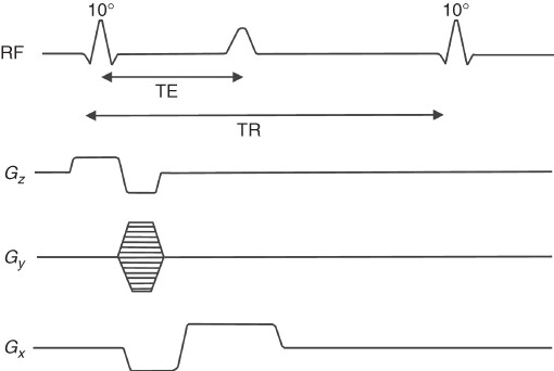
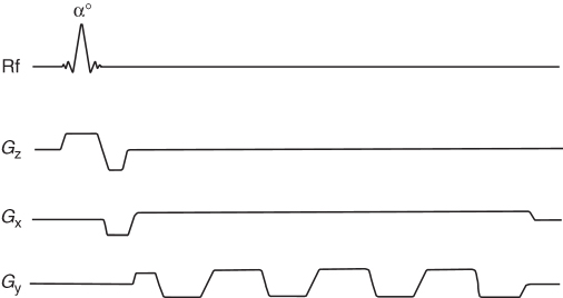
Figure 5.18 Gradient echo echo planar imaging (GE–EPI) pulse sequence: Gz, slice selection gradient; Gx, frequency encoding gradient, and Gy, phase encoding gradient.
The application of a single low flip angle pulse per repetition in GE allows the collection of an image in the order of a few seconds, which is much faster than SE. The first description of GE, including an application of the gradients and low flip angles to obtain a fast image was presented by Hasse in 1989 (26) and called FLASH (Fast Low Angle Shot). This sequence uses so-called spoiling gradients and/or rf spoiling (27) after the acquisition of the echo to destroy the transverse magnetization before the next excitation. When balanced (refocusing) gradients instead of spoiling gradients are used to keep magnetization tilted by the same angle throughout the pulse sequence using the series of rf pulses, the sequences are the so-called Steady-State Free Precession (SSFP) (28). Pulse sequences based on SSFP are, for example, Gradient Refocused Acquisition in the Steady-State (GRASS) or Fast Imaging with Steady-State Precession (FISP or True-FISP) (29, 30). FISP is more sensitive to T2 than the standard GE pulse sequence, which is mostly T2* sensitive.
5.8.1 EPI
The fastest MRI technique, echo planar imaging (EPI), was first introduced by Mansfield in 1977 (31). In the standard version of this technique (single-shot GE-EPI), spins are excited only once (Fig. 5.18), which allows an MR image to be obtained within 50–100 ms. Because GE is used, this pulse sequence is T2* or PD (very short TE) weighted. Very short TE (order of 2–5 ms) can be used. This technique uses low rf power (low flip angle) and very rapidly switching gradients, which create significant acoustic noise due to the gradient coil vibrations. Because the spins are excited only once, there must be enough echo signal available throughout the entire sequence. Therefore, very good shimming of the magnetic field to prolong T2* has to be achieved before the execution of the sequence, as the amplitude of echoes decreases with T2*. The T2* decay also reduces the resolution of EPI in comparison to SE or GE. The image resolution can be increased using multiple-shot EPI, but at the expense of an increased scan time. Since in EPI, spins are excited only once (single-shot EPI), EPI is T2 (SE-EPI) or T2* (GE-EPI) weighted. There is also some PD weighting that depends on the TE value; the shorter the TE the more PD weighting and less T2 and vice versa: longer TE, more T2 and less PD weighting.
To reduce T2* decay effect and the noise generated by the gradient coils, so-called spiral EPI (32) was introduced. The sequence uses sinusoidal gradient waveforms with increasing amplitude in phase and read directions, that creates a spiral trajectory in the k-space (hence the name).
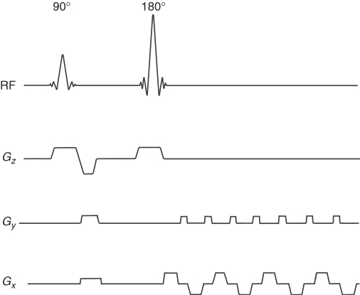
The modification of EPI, SE-EPI, uses 90° and 180° pulses followed by switching gradients as shown in Figure 5.19. In this way, T2 weighting is introduced to EPI.
Figure 5.19 Spin echo echo planar imaging (SE-EPI) pulse sequence: Gz, slice selection gradient; Gy, phase encoding gradient; and Gx, frequency encoding gradient.
5.8.2 FSE
Another commonly used pulse sequence is the Fast Spin Echo (FSE), which uses a series of 90°–180°–180°–180°–… selective rf pulses, similar to the CPMG pulse sequence (Fig. 5.10), along with the appropriate gradients. Each 180° pulse allows collection of an SE, which thus speeds up the acquisition. For instance, for an Echo Train Length (ETL) of 8, only 256/8 = 32 repetitions are needed, instead of 256. FSE is very significant clinically because it allows strong T2 weighting in a short acquisition time. Recall that for SE both long TR and TE are required for T2 weighting—this is slow. FSE can achieve a very long TE for the later echoes in the train, and also a very long TR, as the number of repetitions is reduced by the factor ETL, decreasing the overall acquisition time drastically.
5.8.3 Inversion-Recovery
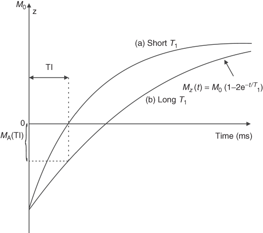
Inversion Recovery (IR) is an alternative method for the introduction of T1 image weighting. It involves the application of a 180° inversion pulse before the imaging sequence (Fig. 5.20), followed by a variable interval called the Inversion Time (TI). The effect of the inversion pulse is to flip all spins to the − z axis. The spins then relax back toward the + z axis with time constant T1. At some point, they must pass though the origin, that is, zero Mz. This is known as the null point. If the 90° excitation pulse (for any sequence) is applied at this point in time, then spins at the null will not be excited and will appear black in the image. In this way, unwanted signal (e.g., from tissue A) can be suppressed. In practice, tissue A is usually blood or fat.
Figure 5.20 Return of magnetization after 180° pulse for the tissue with short (A) and long (B) T1. Magnetization after inversion time (TI) for tissue with short T1 is zero (MA(TI) = 0), but there is a net magnetization for tissue with long T1:MB(TI) ≠ 0. An imaging sequence may start after time TI to avoid signal from tissue A.
There are many combinations of IR with other imaging techniques. Fast inversion recovery is a combination of IR and FSE and allows T1 and/or T2 weighting depending on the selected parameters. STIR (Short Ti Inversion Recovery) is used mostly for fat suppression and applies short TI (100–200 ms) to null the signal from fat, as TI is comparable to fat's T1. To suppress signal from fluids that have long relaxation times ( ∼ 2 s), such as Cerebrospinal Fluid (CSF), TI corresponding to T1 of CSF is selected. Therefore, a pulse sequence with a long TI (over 1500–2500 ms) called Fluid Attenuated Inversion Recovery (FLAIR) (33, 34, 35, 36) is frequently used for brain and spinal cord imaging to null bright CSF.
5.8.4 DWI
In some diseases, for example, stroke, water diffusion is reduced because of cell swelling and their disruption; therefore, diffusion-weighted (DW) MRI is often used (37, 38). DW-MRI can be added to most standard pulse sequences by adding diffusion-sensitizing gradients along one or more directions (depending on the application). The principle is that if a pair of gradients is used, first a dephase gradient, followed after a delay by a rephase gradient, then all static spins will see no net effect. However, moving spins will be at different locations for the two pulses, so will not fully rephase. For random motion (i.e., diffusion), this results in signal loss due to the partially randomized spin phases. The signal reduction depends on the diffusion speed of the spins, amplitude, and duration of the gradients. To obtain stronger diffusion weighting, stronger and/or longer duration gradients must be used.
For SE sequences, DW is implemented by adding two identical gradient pulses, one before and one after the 180° pulse. For GE sequences, a positive polarity pulse is followed by a negative polarity one. Areas of reduced diffusion, such as stroke, appear bright in DW-MRI.
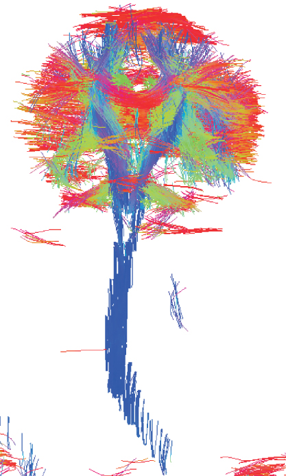
While standard DW-MRI techniques suffer from motion artifacts, the recent application of fast imaging (EPI) along with high magnetic field (3 T and above) can generate fast, high quality DW-MRI. Moreover, multiple diffusion weightings in different directions can be measured to study the directionality of diffusion. The three gradients x, y, z may be combined to create a gradient along combined directions, for example, x-z or x-y. This is the basis of Diffusion Tensor Imaging (DTI) technique, which shows diffusion coefficients in nine directions. Because neurons exhibit faster diffusion along the nerve fibers that surround tissues, points along the maximum diffusion can be connected in three dimensions, using a software program, to create fiber tracking MRI showing spatial distribution of neuronal tissues in brain and recently in spinal cord (Fig. 5.21).
Figure 5.21 Fiber tracts of the human brain and cervical spinal cord. Red color represents fibers running left-right, green represents fibers running anterior-posterior, and blue represents fiber tracts running inferior-superior (3 Tesla Siemens Trio, IBD/NRC, Winnipeg, MB, Canada).
5.8.5 MRA
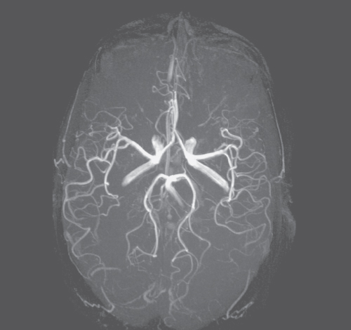
The ability of MRI to measure flow (39) is used in Magnetic Resonance Angiography (MRA) to visualize vasculature, arteries and veins (Fig. 5.22) (40, 41). There are two basic MR methods that make MRI flow sensitive: Time of Flight (TOF) (42, 43) and Phase-Contrast (PC) MRA (44, 45).
Figure 5.22 MR angiography at 3 T (Siemens Canada).
TOF MRA usually uses a GE pulse sequence with short TR and TE. It uses to its advantage the fresh, full magnetization flowing into the imaged slice, which is larger than the magnetization of the stationary spins. The short TR (shorter than T1 of the stationary tissue) does not allow the stationary spin to fully recover; therefore, fresh, in-flowing spins have a stronger signal and appear bright.
PC MRA is accomplished by including bipolar gradients in the pulse sequence: a pair of gradients of the same amplitude but opposite direction is applied one after another. Such gradients affect only the phase of moving spins. This technique, unlike TOF MRA, is sensitive to both incoming spins and spins flowing within the imaged area.
There are 2D and 3D versions of MRA. To obtain a 3D image of blood vessels, a postprocessing method called Maximum Intensity Projection (MIP) is used. The MIP method combines multislice 2D data into one 3D data set by assuming that the strongest signal comes from the vessels. Multiple projections of only the areas of maximum signal (41) onto the image are performed, creating a 3D image of blood vessels. This 3D dataset can then be visualized from different angles by rotation.
To improve the quality of MRA, contrast agents to reduce T1 of the blood are often used, allowing short TR and increasing the blood signal. This technique is called contrast-enhanced MRA (46).
5.8.6 Perfusion
An MRI technique called perfusion MRI allows the measurement of cerebral (or other) blood volume (CBV). The technique uses a short T2 intravenous bolus injection (e.g., Gd based) along with a fast T2 or T2* pulse sequence. The flowing contrast agent causes a transient decrease in the signal from the blood vessels. Data postprocessing analyzes the decay in the signal with time to calculate the volume and speed of the blood. This information is particularly useful in ischemia or in diseases causing metabolic disorders.
Other MRI techniques, still under development, allow for temperature and elastic properties of the tissue to be imaged.
5.9 Enhanced Diagnostic Capabilities of MRI—Contrast Agents
Abnormal tissues are observed with MRI mostly because of their different relaxation times in comparison to healthy tissues. However, the differences are often too small to be readily detectable. To increase the difference, and thus improve CNR, agents that decrease T1 and/or T2 are used. They decrease the tissue proton relaxation times because of their paramagnetic properties, which cause enhanced magnetic field fluctuations in their vicinity, which act to increase proton relaxation. Contrast agents are injected intravenously ( ∼ 0.1 mmol/kg). Because tumors have better vasculature than the surrounding tissue, the density of contrast agents is higher within the tumor. This causes a stronger decrease in the relaxation times within the tumor and results in better tumor contrast. Contrast agents are also particularly useful in the diagnosis of CNS tumors, as they pass through the ruptures in the Blood–Brain Barrier (BBB).
The most common contrast agents are gadolinium(Gd) based. Because Gd ions are toxic if used without a shell, chelates, such as Diethylene Triaminepentaacetic Acid (DTPA), are used to ensure Gd biocompatibility. Gd-DTPA shortens mostly T1. Other contrast agents, such as iron oxide, shorten T2.
5.10 Molecular MRI
Experimental MRI systems using very high fields (9.4 T and above) allow imaging with in-plane resolution below 20 μm (47, 48). Nonetheless, even this resolution does not allow for true in vivo observation of single cells or molecules. Standard human MRI allows detection of tumors of the order of millimeters in diameter ( ∼ 108 cells) but no smaller.
However, the recent developments in nanotechnology and molecular biology (49, 50) have allowed this limit to be overcome, and cellular or even molecular MRI was recently established. Molecular MRI uses strong paramagnetic or superparamagnetic Nanoparticles (NPs) (such as FeCo nanocrystals) that decrease relaxation times more than standard contrast agents (such as Gd-DTPA). Biologically active entities such as stem cells or antibodies can then be labeled with these NPs and be tracked with MRI. Owing to their strong paramagnetic properties, even small amounts of NPs can allow imaging of small numbers of specific cells, targeted by the appropriate biological vehicles. The development of this method allows the detection of cancer and other diseases at a very early stage, which is extremely important to achieve successful treatment. In addition, NPs used in MRI can also be synthesized with a shell that can be detected with other imaging modalities, such as infrared spectroscopy (Chapter 9), expanding MRI into multimodal diagnostic imaging (49). A very recent study showed that it may also be possible to not only diagnose the disease but also treat by thermoablation of the abnormal tissues using rf-generated heat absorbed by certain types of NPs (51, 52, 53) attached to the target.
5.11 Reading the Mind—Functional MRI
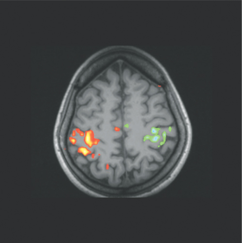
Functional Magnetic Resonance Imaging (fMRI) is a technique that has introduced imaging into new areas of neuroscience, psychology, and clinical applications. fMRI allows for noninvasive, indirect observation of the neuronal activity in the brain (54) and, very recently, in the spinal cord (55, 56). With fMRI, it is possible to dynamically image blood oxygenation levels during the synaptic activity. This mechanism is called Blood Oxygen Level Dependent (BOLD) MRI and was first observed with MRI in 1990 by Ogawa et al. (57). Deoxyhemoglobin (a paramagnetic substance) shortens T2* (and to a lesser extent T2). During brain activation, the amount of oxyhemoglobin increases and deoxyhemoglobin decreases, increasing T2*, detectable as an increase in GE signal intensity. Since the changes in the signal intensity are rather small (2–5%), in order to increase the statistics, an fMRI study usually comprises 2–3 rest and 2 active periods. This pattern of stimulation is called the paradigm. Therefore, subjects under fMRI examination are requested to repeat the task (e.g., finger tapping or a mental task) two or more times. During the fMRI experiments, serial MR images are obtained continuously and at as high a rate as possible. Statistical analysis (58) of the collected images is used to determine voxels of activation, by correlating their signal intensity changes over time with the paradigm. The paradigm for the correlation analysis is usually designed as a ramped step increase/decrease in signal intensity when the stimulation comes on and off during the experiment. Voxels undergoing signal intensity changes that correlate with the defined paradigm (with a correlation coefficient threshold of p ≤ 0.01 or better) are assumed to represent regions of neuronal activation corresponding to the applied stimulation. The activated voxels are then overlaid with a color scale corresponding to level or correlation to the paradigm, onto high resolution anatomical images (Fig. 5.23). To optimize fMRI sensitivity to T2* relaxation, GE or EPI pulse sequences are used with TE ≈ T2* (about 30 ms at 1.5 T).
Figure 5.23 fMRI image showing areas of neuronal activity caused by a movement of the left (red) and right (yellow) hands.
There are other possible mechanisms that may also be involved in fMRI based on changes in diffusion (59) and extravascular proton content (60) during neuronal activation.
5.12 Magnetic Resonance Spectroscopy
MR spectroscopy (MRS) represents a whole new dimension to biological MR. Historically, MRS (or NMR spectroscopy) preceded MRI as a simpler technique ex vivo and found an application in biochemistry in the 1960s. Spectroscopy provides information about the chemical composition of the object studied.
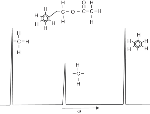
As mentioned in Section 5.2, the Larmor frequency (frequency of the spins rotating in the magnetic field) depends on the strength of the external field. Electrons orbiting the nucleus shift the main field by a few parts per million (ppm). Thus, the frequency of the nuclei depends on the local electron environment, that is, on the position of the nuclei within the molecule, in other words, on the chemistry. For this reason, this effect is called chemical shift (δ), and it is the principle that gives MRS the ability to locate MR-sensitive atoms within a molecule. Because each compound has a unique chemical structure, its MR spectra can be used for identification. For example, the spectra of benzyl acetate C6H5CH2COOCH3 (Fig. 5.24) reveals three peaks corresponding to the three different proton locations within the compound. The amplitude of the peaks corresponds to the number of protons within the compound. Note the smaller peak in Figure 5.24 from CH2 (two protons), relative to CH3 (three protons).
Figure 5.24 MR spectrum of benzyl acetate. The peaks correspond to different positions of 1H in the compound.
In vitro MR spectra are obtained by applying an rf pulse (usually nonselective 90°), followed by FT of the collected data. No gradients are required. The stronger the external field, the easier it is to separate peaks in the spectra, therefore the use of strong magnets (up to about 20 T) for high resolution spectroscopy. Critical, however, is making the main field as homogenous as possible (so-called shimming), as the FID decreases faster with the field inhomogeneities and the spectral signals (lines) become broader and overlap. To be able to identify spectra independently of the strength of the external field, chemical shift (δ) is expressed in ppm as ![]() , where ωcalib is the Larmor frequency of the external marker (usually water) and ω0 is the frequency of the spectrometer.
, where ωcalib is the Larmor frequency of the external marker (usually water) and ω0 is the frequency of the spectrometer.
MR spectra used as a “fingerprint” of a compound allows identification of metabolites and monitoring of metabolic processes in tissues. As the content and the ratio of specific metabolites, such as choline, creatine, N-acetyl-aspartate (NAA), glucose, or lactate, change with pathology (e.g., in cancer or stroke), MRS can be used to identify the disease (61) or its stage. The same principles apply to other NMR nuclei; however, their MR sensitivity is usually lower than 1H, thus a longer acquisition time is needed to collect valuable data. Of particular interest is phosphorus (31P), which is important in energy storage and energy exchange processes within cells. For example, 31P MRS shows changes in the ratio between Phosphocreatine (PCr) and Inorganic Phosphate (Pi) during muscle exercise, as well as the shift in the peaks frequency due to changes in pH (62). The ratio PCr/Pi can be diagnostic, as it varies in certain diseases (64).
5.12.1 Single Voxel Spectroscopy
Single voxel localized MRS allows the collection of MR spectra from a selected region of interest (voxel) within a patient. To define the voxel, three selective pulses, along with slice selection gradients, are applied in three directions. The signal is collected from the spins in the intersection of the three planes. The two most common of these methods are Stimulated Echo Acquisition Mode (STEAM) and Point Resolved Spectroscopy (PRESS). STEAM uses stimulated echoes to collect the data (63, 64). PRESS uses SEs and results in double the signal strength in comparison to STEAM (65).
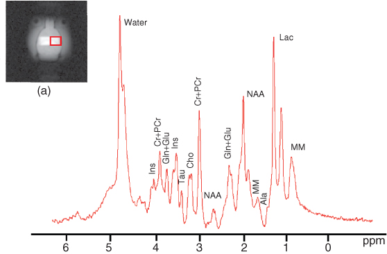
MRS requires very good field shimming before the collection of data. An example of an in vivo spectrum from a selected voxel at 9.4 T is shown in Figure 5.25. In practice, because spectral resolution and SNR increases with the field, MRS benefits greatly from higher field strengths (3 T or higher); however; it is not uncommon to see good spectra at 1.5 T.
Figure 5.25 MR spectrum of metabolites from VOI shown in (a) at 9.4 T using STEAM.
5.12.2 Spectroscopic Imaging
An interesting combination of MRS and MRI is MR Spectroscopic Imaging (SI or MRS imaging) or Chemical Shift Imaging (CSIs). SI shows the spectra from each voxel (usually 16 × 16 or 32 × 32) overlaid on anatomical MR images. In this way, observations of differences in metabolite content between, for example, left and right hemispheres, or abnormal spectra in dubious areas, can be made and used for enhanced diagnosis. A disadvantage of SI is the long time required to collect data from all, usually small ( ∼ 5 mm × 5 mm × 5 mm), voxels. The distribution of a selected metabolite within the subject may be displayed as an image. This is achieved by selecting a particular peak of the spectrum from each voxel, calculating the total area under that peak and assigning a pixel intensity or color at each point.
5.13 MR Hardware
To the patient, CT and MRI systems look much alike—resembling a tube or ring. However, this is the only similarity between the techniques, as both the principles and equipment are very different.
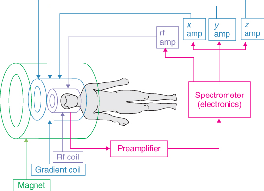
As described in the previous sections, to obtain an MR image, an external static, variable magnetic gradients, rf field, data acquisition, and postprocessing are all needed. To achieve all this, each MRI system consists of a set of subsystems with distinct functions: magnet and shim system, gradient system, rf system, and the user interface and control system. Alternatively, the system can be broken down by physical assemblies: magnet, gradient coils, rf coils, power amplifiers, and console. The schematic diagram of an MRI system is shown in Figure 5.26. The components are described in detail by Chen and Hoult (66).
Figure 5.26 Schematic of major components of an MRI system.
5.13.1 Magnets
The basic parameters of a magnet are the strength of the magnetic field (expressed in tesla (SI) or Gauss; 1 T = 10, 000 Gs), the homogeneity of the field within the Volume of Interest (VOI) (ppm over Diameter of Spherical Volume (DSV)), and the fringe field that describes the distribution of the field around the magnet. The edge of the fringe field is usually defined at the 5 Gs line. This denotes the distance from the center of the magnet to the location where the field has fallen to 5 Gs.
MR magnets must generate a field stronger than 0.1 T. Currently, most clinical systems generate 1.5 T. However, human 3 T magnet systems, which recently obtained FDA approval, are more and more common. Seven-tesla whole-body magnets are used in human research systems, and even higher field whole-body systems are under construction. Experimental animal systems, with a magnet bore of 30 cm or less, are usually equipped with magnets of 4.7 T (200 MHz), 7 T (300 MHz), 9.4 T (400 MHz), and 11.7 T (500 MHz) (Fig. 5.27), whereas stronger (14 T) magnets are under construction. Magnets generating a magnetic field of 20 T or above are used for ex vivo MRS. Stronger magnets are not common yet not only due to the technical challenges associated with the construction of magnet but also due to safety issues. There are three types of magnets used in MRI depending on the manufacturing process: permanent, electromagnets, and superconductive.
Figure 5.27 Vertical experimental 11.7-T MRI system (IBD/NRC), magnet (Magnex Scientific, England), and console (Bruker, Germany). (b) 3-T Siemens Trio MRI system.

The majority of human and all high field experimental MRI systems are equipped with superconductive magnets. These can produce very stable and strong magnetic fields up to about 20 T. Their shape usually resembles a vertical (Fig. 5.27a) or horizontal (Fig. 5.27b) cylinder. All human and most animal MRI systems are horizontal. The most important geometric parameter of the superconductive magnet is the diameter of its inner tube (“the bore”) of the magnet. Shimming coils, gradients coils, and body rf coils (in humans systems) are placed within the bore of the magnet.
Construction of superconductive magnets became possible following the discovery of the phenomenon of superconductors, which carry electrical current without any resistance. Superconductive materials (e.g., alloy niobium–titanium) have no resistance at a very low temperature ( ∼ 4 K). Superconductive magnets are made of many turns of superconductive solenoidal wire, submersed in liquid helium at its boiling point of a temperature of 4.2 K ( − 269°C). The magnet is charged with an electrical current of hundreds of amperes into the superconductive wire. As long as the wire is submersed in liquid helium, the current remains constant—forever. To prevent excessive boiling, the liquid helium is separated from the warm air in the magnet room with layers of liquid nitrogen (77K = − 196°C) and vacuum. Most magnets produced before the year 2000 require filling with liquid hydrogen every 5–6 weeks and with liquid helium every few months. However, most twenty-first century magnets are equipped with helium cryocoolers, thus liquid nitrogen is not required. Should the liquid helium level become too low, the magnet may disastrously and expensively “quench,” as the wire temperature becomes too high to sustain superconductivity. The wire becomes resistive, generating a large amount of heat, causing rapid helium boiling and evaporation. So each system must be also equipped with a fat quench line to vent the helium gas outside to prevent oxygen depletion in the magnet room.
Human superconductive 1.5- and 3-T magnets, with bore diameter of about 1 m, despite so-called active shielding (superconductive wires around the main wire restraining the outside field), have a rather large fringe field: the 5-Gs line extends about 2–4 m from the center of the magnet. This can be a distinct siting issue for 3-T magnets in particular. At the time of writing, large bore magnets over 4 T are not actively shielded; thus, their fringe field is much larger (order of 10 m). In that case, an iron cage around the magnet is often used to reduce the fringe field. The price for the MRI system based on a superconductive magnet is roughly $1M per 1 T, that is, a 1.5-T system costs about $1.5M.
Permanent magnets are constructed with hundreds of brick-shaped (about 5 cm × 5 cm × 10 cm each), very strong permanent magnets, supported by a steel structure with high magnetic permeability, which becomes part of the magnetic circuit. The small magnets are made of iron-rare-earth elements (Nd-Fe-B). The shape of the magnet is usually four post (Fig. 5.28) or C-shaped. The supporting steel structure and the posts (or the arm) shape the magnetic field created by the small magnets. Owing to the open design, children and claustrophobic patients can be imaged with less stress. Motion of joints (e.g., knee) can also be easily imaged because of the legroom afforded by the open design. The maximum field for human imaging is 0.35 T, so the acquisition time required to obtain an MR image of 1.5-T quality is much longer. However, for many practical applications, the exquisite 1.5-T image quality is unnecessary, and permanent magnet systems are a viable alternative. Recent advantages in pulse sequence development such as parallel imaging, allowing decrease of the acquisition time, however, make permanent magnets more appealing. The fringe field is very small, and a 5-Gs line is usually about 0.5 m from the magnet's edge. Permanent magnets are maintenance free, as they require no power supply or cryogens to operate; however, their weight is about 10 tonnes (10,000 kg). As the field strength of permanent magnets drifts down with increasing temperature, thermal stabilization (about ± 1°C) or field drift compensation systems are required in the magnet room. Modern air conditioning systems can easily meet this requirement. Field compensation system, called B0 compensation, is also simple to implement by using an additional pair of circular wires on magnet poles.
Figure 5.28 A 0.2T four-post MRI system (MRI-Tech, Canada).
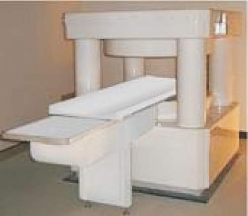
Electromagnets (resistive magnets) are rather uncommon in MRI. They use conductive wires to produce the magnetic field and generate fields up to 0.5 T. They require huge amounts of electrical power provided by a water-cooled power supply. As small variations in the wire current cause changes in both the field strength and homogeneity, dedicated field stabilization systems are needed. Short-term instabilities can be dealt with by flux stabilizers, while long-term drift is minimized using additional field coils.
5.13.2 Shimming
Shimming is the process of fine-tuning the magnet field uniformity. There are three methods: passive, active with resistive coils, and active with superconductive coils.
The use of iron pieces for shimming is called passive shimming and is used for shimming to about 10 ppm. Washer-like iron pieces of about 1-cm diameter are placed on both poles of the magnet in very specific locations, as determined by computerized field analysis.
For high field human MRI, the homogeneity should be about 10 ppm over 30–50 cm DSV, while for MRS, local homogeneity should be in the order of 1 ppm over a voxel volume. (It can be proved that for MRS the variation in field frequency should not be larger than 1/πT2 over the sample volume (67).) Although superconductive magnets produce highly uniform fields, homogeneity improvement of the field is often needed. Passive shimming, using iron pieces placed on the inner surface of the bore of the magnet, is used. Superconductive wires (cryoshims) submersed in liquid helium are also used in some magnets for active shimming. The shims are charged after the main wire is charged.
As a sample or a subject changes the magnetic field because of their magnetic properties, additional shimming is often needed before each imaging session. This fine shimming is accomplished by resistive, Room Temperature (RT) shims. These shims are usually incorporated into the gradient coils on their external surface. As each field can be mathematically expressed in spherical harmonics, the process of shimming aims at the minimization of specific harmonics, denoted as x, y, z, 2xy, z2 − y2, and so on. RT shims are particularly useful in MRS and multiecho pulses (such as GE-EPI), as they are very sensitive to any field inhomogeneity.
A permanent magnet has a “raw” homogeneity of about 300–500 ppm over 30–50 cm DSV. Passive shimming allows improvement of homogeneity to about 10 ppm. Of course, there are no cryoshims available for permanent or electromagnets.
5.13.3 Rf Shielding
The NMR signal is very weak, so the magnet is placed in an rf-shielded room to prevent any external rf interferences that could cause spurious signals to be detected by the system. The shielding efficiency should be about 100 dB. There must be special conductive doors installed to make sure that the room is “rf sealed” during imaging. All cables coming into and out of the magnet room must go through an rf filter panel to block unwanted signals, while nonconductive tubes may go through waveguides that prevent rf leakage.
5.13.4 Gradient System
Gradients provide spatial information in MRI. The gradient system consists of: waveform generation, gradient power amplifiers, high power cables and filters, and finally the gradient coils within the magnet. To generate a time-variable gradient, needed for spatial spin encoding, the magnetic field gradient coils are made of resistive wires overlaid on the surface of a fibreglass tube. As three perpendicular gradients are needed, usually six layers of wire are used: three inner layers generating gradients within the VOI and three layers used as a magnetic shield to prevent eddy currents being induced in the cryostat. Of course, each layer must be electrically separated and water or air cooling must be provided, as large currents are generated when gradients are working. The gradients are wired on the surface of a fibreglass tube and immobilized and electrically separated with an epoxy resin or a similar substance. The tube is then placed inside the bore of the magnet. Important parameters of the gradients coils are linearity over VOI, efficiency, maximum strength, and rise time or slew rate. The linearity defines how constant the gradient is over the VOI (usually better than 5%). This is a very important parameter, as any deviation from linearity distorts an image. The maximum gradient produced by the gradient coils can be calculated by multiplying the coil efficiency (in mT/m/A) by the maximum current provided by gradient amplifiers. Modern MRI clinical systems provide a maximum gradient of about 40 mT/m, while experimental MR systems provide gradients over 1000 mT/m. Gradient amplifiers generate hundreds of amperes and hundred of volts. Minimum rise time is the minimum time required to achieve maximum gradient amplitude. This time varies from system to system and depends on inductance and resistance of the coil and the gradient amplifiers used. In clinical systems, minimum rise times vary from 100–500 μs, while it is less than 100 μs in experimental MR systems. Another frequently used parameter is the slew rate, which combines maximum gradients strength and their rise times, expressed in mT/m/s.
5.13.5 MR Electronics—The Console
The rack of low power electronics and the computers used to run the system is termed the console. A typical breakdown of a console would be into a Graphical User Interface (GUI), a synchronous high speed control assembly, and a low speed asynchronous control assembly.
The main tasks of the high speed synchronous control are to generate the gradient, rf, and timing waveforms and to acquire and digitize the NMR signals. Modern systems may have a large number of receiver channels, such as 32. Low speed control is used for tasks such as configuration of gains, switches, shim currents, temperature monitoring, and so on.
There is no console standardization in the industry—each major and minor manufacturer, both clinical and otherwise, have their own designs. Thus, it can be a major task to transfer experience from one to another. On the bright side, however, all clinical manufacturers do comply to a standard clinical image data format (DICOM).
The three largest commercial suppliers of human MRI systems are GE, Siemens, and Philips. Two major suppliers of experimental MRIs are Bruker and Varian. There are many smaller suppliers around the world.
Most commercial MR consoles are based on dedicated and sophisticated computers. However, recent progress in personal computers allowed their application to MRI. A few smaller commercial suppliers (e.g., ONI Corp, Maran (Oxford Instruments)) and even research institutions have created systems based on PCs. For example, the National Research Council of Canada has designed a console system that integrates simulation of the MR experiment with the acquisition of experimental data. The device consists of a magnetic resonance (MR) research console with a full-function hardware-independent pulse programming environment and a parallel computer cluster running Bloch equation MR physics simulations on a 3D digitally defined spin phantom. The system is designed to allow precise side-by-side comparisons of experimental against theoretical predictions for real world, complex pulse sequences and is in operation on both 0.2T and 9.4 T systems (67).
5.13.6 Rf Coils
The rf coils (rf probes) generate the rf (B1) pulse fields and receive the MR signals. The basic construction principles are simple, based on the L-C resonance circuit. There are transmit (Tx)-only, receive (Rx)-only, and combined transmit and receive (Tx/Rx) rf coils. Most clinical systems are equipped with a Tx-only large rf coil (body rf coil) and a selection of local Rx-only coils. The parameters of the rf coil are B1 (rf) field homogeneity, quality factor (Q), and the coil's FOV. MRI and MRS require both maximal SNR and homogeneous B1 field. Unfortunately, these requirements usually conflict: the better the SNR the worse the B1 and vice versa.
An inhomogeneous B1 transmit field causes variations in the MR image intensity because of the spatial dependence of the flip angles (compare Eq. 5.2). This is particularly inconvenient when more than one pulse is used for MRI or MRS. In quantitative MRS, metabolite concentration cannot be properly evaluated when the rf coil produces an inhomogeneous B1 field. Therefore, the application of rf coils producing a spatially uniform B1 field is preferred.
The best SNR is produced over a small FOV by a local (surface), single loop coil (Figs 5.29c and 5.30), which, however, produces a very inhomogeneous B1 field, dropping rapidly with distance from the coil. Various designs of small Rx-only coils are used for particular body parts such as the knee, arm, or head.
Figure 5.29 Inner structure of rf coils. (a) Birdcage, (b) surface, (c) inductively coupled Helmholtz pair (NRC, Canada).
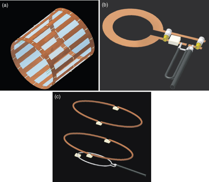
Figure 5.30 Examples of rf coils. (a) Breast coil (IBD/NRC), (b) solenoidal volume coil (IBD/NRC), (c) surface coil (IBD/NRC), (d) head coil (Siemens, Germany), and (e) phase array torso coil (Siemens, Germany).
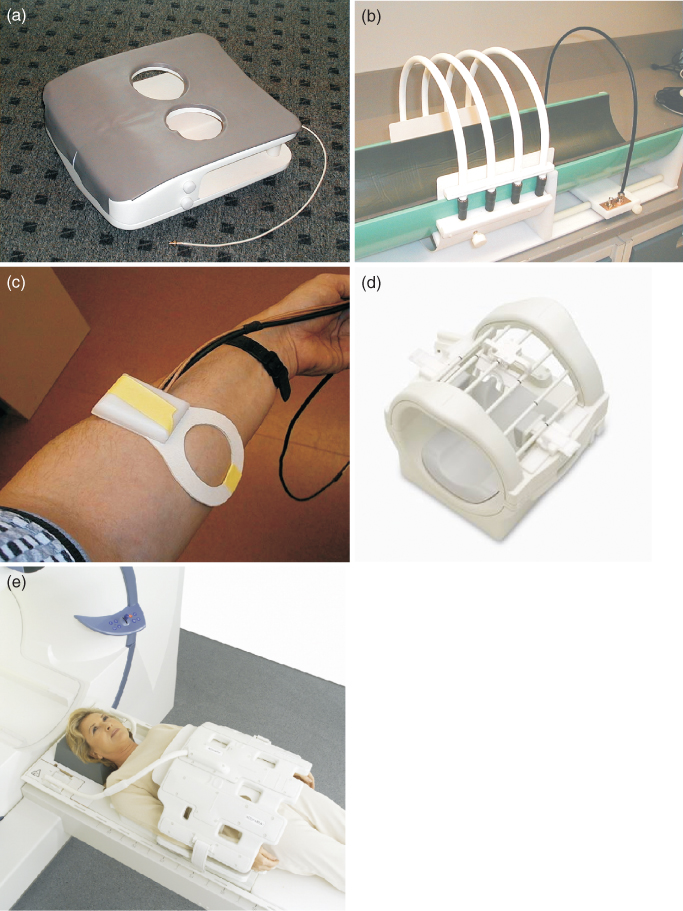
Volume coils produce a homogenous B1 field over a large area, such as the body or the head. The most common volume coils are saddle coil, the solenoidal coil, the Alderman-Grant, the Helmholtz pair, and birdcage (Fig. 5.29). Unfortunately, they suffer from low sensitivity (as receiver coils) and high power requirements (up to 30 kW) compared to the surface coil (68). Examples of various rf coils are shown in Figure 5.30.
Coil sensitivity depends on the geometry, quality factor (Q), material used for the coil construction, electric circuit used to couple the coil (inductive or capacitive), filling factor of the coil (ratio between the volume of B1 and the volume of the imaged object), and type of polarization (linear or circular).
Almost all volume coils and some surface coils use quadrature detection (so-called Circular Polarized (CP) coil) (70, 71). The quadrature detection allows SNR increase by up to √2 when compared to the Linear Polarized (LP coil) coil. The quadrature rf coil requires the creation of two equal and orthogonal B1 fields. This can be easily achieved in the birdcage coils using proper driving system and two of its modes. The quadrature coil requires less power when compared to the LP coil.
Surface coils produce high SNR but within limited FOV. To extend the FOV over the sample a phased array technology was introduced (71). Each element of the array, coupled to an independent receiver channel, works as an independent surface coil maximizing SNR and increasing FOV.
Advanced MRI systems allow multinuclear studies to be performed. Quantification of tissue metabolites by heteronuclear MRS can be achieved using dual-frequency rf coils. The dual-frequency coils allow simultaneous measurement of two nuclei frequencies, such as 1H and phosphorus (31P). The proton signal is usually used for high resolution imaging, whereas the other frequency is used for spectroscopy. The proton frequency also provides the sensitivity needed for shimming. Dual-frequency coils have to deliver the SNR of the single-frequency rf coil as well as produce homogenous rf field over the sample volume. To achieve these needs, double-tuned quadrature birdcage coils were developed (72).
5.14 MRI Safety
MRI is a noninvasive imaging technique with no long-term side effects observed. However, there are a few potential safety issues that should be considered when working with MRI systems or as a subject of MR examination: static magnetic field, rf power absorbed by the subject, and variable gradients of the magnetic field.
5.14.1 Magnet Safety
While long-term effects of the static magnetic field on living organisms have not been observed, the FDA, as a precaution, set up a limit of 3 T for human clinical MRIs. Other countries followed that limit. Potential subtle, long-term biological effects aside, there is always an immediate danger—projectiles.
Magnetic fields attract ferromagnetic objects, such as oxygen tanks, scissors, carts, computers, and so on. Such objects can become projectiles and injure or kill anyone between the magnet and the object. Therefore, there must be no ferromagnetic objects within the 5-Gs line. Some surgical clips, prosthesis, and implants may also be attracted by the magnet. However, some of them, made of nonferrous material, are MRI compatible and can be safely imaged. Nonetheless, in most cases they create artefacts in MR images. Of course, under no circumstance can patients with pacemakers be imaged. It is considered that the region outside the 5-Gs line is safe for practically all objects, including cardiac pacemakers, but it may be worth to remember that magnetic cards (such a credit card or hotel magnetic key) may be erased by the field around 5 Gs.
In very rare cases, moving in the magnet may cause a temporal discomfort, depending on the individual's sensitivity, because of the eddy currents induced in the brain due to the motion in the magnetic field.
Clinical MRI systems are equipped with rf power amplifiers capable of generating up to 30 kW rf power in short pulses, which heat up tissues and can be potentially harmful. Therefore, the regulations do not allow the use of rf power that would heat the tissue by more than 1°C. However, this definition is not convenient in MRI; therefore, Specific Absorption Rate (SAR) is used. This is defined as rf power absorbed in tissue per unit mass, and is expressed in watts per kg (W/kg). The SAR limits vary from 3 W/kg to 12 W/kg depending on the total exposure time and on the part of the body. Clinical MRI systems calculate the SAR value before the pulse sequences are run and lock-out the imaging in case SAR exceeds the allowed value. It also should be noted that SAR increases with B02 for fields below 4 T.
5.14.2 Gradient Safety
Gradient coils produce a time-varying magnetic field (dB/dt) that can cause peripheral nerve stimulation and involuntary muscle contraction. Therefore dB/dt is also limited.
In addition, fast switching current in the gradient coils causes acoustic noise due to coil vibrations, which depends on the pulse sequence used. The more demanding the pulse sequence from the point of view of the gradient strength and rise time, the noisier the sequence is. Therefore, fast pulse sequences such as EPI are usually very noisy. However, spiral EPI, which reduces the gradients' rise time, makes the sequence quieter. DW-MRI is also often noisy because of strong diffusion gradients. Because the gradient strength required increases with the field strength, the stronger the magnet, the noisier the pulse sequences are. But this is also the reason why there is practically no noise in low field MRI, such as 0.2 T.
5.15 Imaging Artefacts in MRI
MRI allows imaging of many different tissue properties depending on the technique used. The variety of techniques is possible because of the sensitivity of MRI to different phenomena. This sensitivity, however, may cause a lot of artefacts due to the hardware imperfections, improper pulse sequence tuning, or some external factors. Hardware imperfections may include inhomogeneous main field, nonlinear gradients, inhomogeneous rf field, or eddy currents induced in the cryostat, to mention a few. Improper optimization of pulse sequences may cause a lot of artefacts depending on the pulse sequence used, for example, multiecho pulse sequences may produce unwanted stimulated echoes, improper rf spoiling or refocusing may create unwanted MR signals, etc. The most common artefacts are susceptibility artefacts, flow, phase wrapping (aliasing), or motion ghosting. Phase wrapping occurs when the FOV is smaller than the object size along the phase encoding direction, because of the impossibility of distinguishing between ϕ and ϕ + 360° phase of the signal. This artefact manifests itself when a part of an image shows on the opposite side of the imaged object. The FOV is increased to rectify this problem.
However, there is no good remedy for the susceptibility artefact caused by the variation in the magnetic field between two different tissues or image objects, such as lungs and blood or bone and implants. The images can be badly distorted in such areas, especially for sensitive sequences such as EPI.
Motion artefact (ghosting) is the most common artefact caused by the motion of the subject during data acquisition. It is observed as a blurring or multiplication of the object, depending on the degree of movement, along the phase encoding direction, due to phase misregistration. The remedy is obvious but not always possible, as not all patients can stay motionless for the imaging session. This is particularly important in fMRI, when series of images are compared and any misregistration can lead to incorrect data analysis; therefore, software programs are used to realign the images.
Flow artefact may cause areas of flowing spins to enhance or reduce image intensity. Artefacts from pulsatile flow in arteries may also cause periodic ghosting.
5.15.1 High Field Effects
Serious problems with image homogeneity and SAR occur when the size of the imaged object becomes comparable with the half wavelength (in this object) of the rf field used for imaging. This occurs, for instance, for whole-body imaging at field strengths above 3 T. As described and explained by Hoult (73), even a perfectly made rf coil, producing a homogenous rf field, will not provide a homogeneous image because of this interaction between the rf field and the tissue. As a result, images may be, for example, dark in the center and bright at the edges, or vice versa, depending on the power of the rf pulse used. Maybe of even more importance than image inhomogeneities, is the local SAR that may exceed SAR limits in certain areas of the body, because of the uneven distribution of the electrical field. This problem is a major challenge in very high (>3 T) human MRI. One approach to deal with this problem, the use of multiple transmit systems, was recently introduced (74) and is a subject of research.
5.16 Advanced MR Technology and Its Possible Future
A major direction in MR technique development is the reduction of imaging time without any decrease in image resolution. Probably the biggest advancement in this area recently was triggered by the introduction of the parallel imaging technique (75, 76, 77, 78). This is a technique requiring MRI systems equipped with multiple receivers. Parallel imaging works by using knowledge of the spatial sensitivity response of multiple receiver coils to decode under-sampled data to produce images.
There are two basic approaches to parallel imaging with different mathematics, but which fundamentally achieve the same result. They are the Simultaneous Acquisition of Spatial Harmonics (SMASH) (75) and its modifications, Sensitivity Encoding (SENSE) (77) and Generalized Autocalibrating Partially Parallel Acquisitions (GRAPPA) (78). Parallel imaging allows reduction of the acquisition time without any loss in data-acquisition efficiency.
The challenges associated with image homogeneity at high field spurred the development of multi-transmit systems (transmit array), which allow control of both phase and amplitude in each independent transmit channel. While such a design has been primary used for B1 shimming it may possibly also be used for new MRI techniques, which can reduce some gradient requirements to obtain an MR image (79). The possible combination of receive and transmit phase array systems, should it be successful, may overcome the image resolution limits caused by the standard way of data collection (with gradients). Such a system of the future may push the resolution limits and at the same time avoid acoustic noise generation and safety issues associated with dB/dt and SAR.
In summary, new MRI techniques, new discoveries, and new applications keep broadening the MRI horizons. The information provided by MRI allows better and better diagnosis, more timely treatments, and better outcomes.
5.17 Acknowledgments
We thank Nancy Anderson and Rudy Sebastian for the great assistance and dedication with drawing the pictures. We also thank Dr Dorota Bartusik for help with literature search.
1. Carr HY, Purcell EM. Effects of diffusion on free precession in nuclear magnetic resonance experiments. Phys Rev 1954;94(3):630–638.
2. Bloch F. Nuclear induction. Phys Rev 1946;70:460–474.
3. Hahn EL. Spin echoes. Phys Rev 1950;80:580–594.
4. Gabillard R. Résonance nucléaire mesure du temps de relaxation T2 en presence d'une inhomogenéité de champ magnétique supérieure à la largeur de raie. C R Acad Sci (Paris) 1951;232:1551–1553.
5. Gabillard R. A steady state transient technique in nuclear resonance. Phys Rev 1952;85:694–695.
6. Damadian R. Tumor detection by nuclear magnetic resonance. Science 1971;171:1151–1153.
7. Mansfield P, Grannell PK, Garroway AN, Stacker DC. Proceedings of the 1st Specialised Colloque Ampere; Krakow, Poland; 1973.
8. Mansfield P, Grannell PK. NMR ‘diffraction’ in solids? J Phys 1973;C6:L422.
9. Mansfield P, Maudsley AA. Proceedings of the 19th Colloque Ampere; Heidelberg; 1976. p.247.
10. Hinshaw WS. Spin mapping: the application of moving gradients to NMR. Phys Lett 1974;48A:87–88.
11. Andrew ER, Bottomley PA, Hinshaw WS, Holland GN, Moore WS, Simaroj C. NMR images by the multiple sensitive point method: application to larger biological systems. Phys Med Biol 1977;22:971–974.
12. Lauterbur PC. Image formation by induced local interactions: Examples employing nuclear magnetic resonance. Nature 1973;242:190–191.
13. Garroway AN, Grannell PK, Mansfield P. Image formation in NMR by a selective irradiation process. J Phys 1974;C7:L457.
14. Hoult DI. Zeugmatography: a criticism of the concept of a selective pulse in the presence of a field gradient. J Magn Reson 1977;26:165.
15. Kumar A, Welti D, Ernst RR. NMR fourier zeugmatography. J Magn Reson 1975;18:69–83.
16. Hoult DI, Saunders JK, Sutherland GR, Sharp J, Gervin M, Kolansky HG, Kripiakevich DL, Procca A, Sebastian RA, Dombay A, Rayner DL, Roberts FA, Tomanek B. The engineering of an interventional MRI with a movable 1.5 Tesla magnet. J Magn Reson Imaging 2001;13:78–86.
17. Westbrook C. MRI at a Glance. Osney Mead, Oxford: Blackwell Publishing Ltd; 2002.
18. Bernstein MA, King KF, Zhou JX. Handbook of MRI Pulse Sequences. London: Elsevier Academic Press; 2004.
19. Liang Z, Lauterbur PC. Principles of Magnetic Resonance Imaging: A Signal Processing Perspective, IEEE Press Series in Biomedical Engineering. New York: IEEE Press.
20. Abragam A. Principles of Nuclear Magnetism. New York: Oxford University Press; 1989.
21. Haacke EM, Brown RW, Thompson MR, Venkatesan R. Magnetic Resonance Imaging: Physical Principles and Sequence Design. New York: John Wiley & Sons; 1996.
22. Bracewell RN. The Fourier Transform (FT) and its Applications. New York: McGraw-Hill; 1986.
23. Ernst RR, Anderson WA. Application of Fourier transform to magnetic resonance spectroscopy. Rev Sci Instrum 1966;37:93–102.
24. Carr HY, Purcell EM. Effects of diffusion on free precession in nuclear magnetic resonance experiments. Phys Rev 1954;94:630–638.
25. Hoult DI, Richards RE. The signal-to-noise ratio of the nuclear magnetic resonance experiment. J Magn Res 1976;24:71.
26. Haase A, Frahm J, Matthaei D, Hänicke W, Merboldt KD. FLASH imaging: rapid NMR imaging using low flip angle pulses. J Magn Reson 1989;67:388–397.
27. Wehrli FW. Fast-Scan Magnetic Resonance: Principles and Applications. New York: Raven Press; 1991.
28. Haacke EM, Wielopolski PA, Tkach JA, Modic MT. Steady-state free precession imaging in the presence of motion: application for improved visualization of the cerebrospinal fluid. Radiology 1990;175:545–552.
29. Oppelt A, Graumann R, Barfuss FisherH, Hartl W, Schajor W. FISP: eine neue schnelle Pulssequenz für die Kernspintomographie. Electromedica 1986;54:15–18.
30. Scheffler K, Henning J. T1 quantification with inversion recovery True-FISP. Magn Reson Med 2001;45:72–723.
31. Mansfield P. Multi-planar image formation using NMR spin echoes. J Phys C: Solid State Phys 1977;10:L55–L58.
32. Ahn AB, Kim JH, Cho ZH. High-speed spiral-scan echo planar NMR imaging. IEEE Trans Med Imaging 1986;MI-5:1–6.
33. Hajnal JV, De Coene B, Lewis PD, Baudouin CJ, Cowan FM, Pennock JM, Young IR, Bydder GM. High signal regions in normal white matter shown by heavily T2-weighted CSF nulled IR sequences. J Comput Tomogr 1992;16:506–513.
34. De Coene B, Hajnal JV, Gatehouse P, Longmore DB, White SJ, Oatridge A, Pennock JM, Young IR, Bydder GM. MR of the brain using fluid-attenuated inversion recovery (FLAIR) pulse sequences. Am J Neuroradiol 1992;13:1555–1564.
35. Rydberg JN, Hammond CA, Grimm RC, Erickson BJ, Jack CR Jr, Huston J III, Rieder SJ. Initial clinical experience in MR imaging of the brain with a fast fluid-attenuated inversion recovery pulse sequence. Radiology 1994;193:173–180.
36. Noguchi K, Ogawa T, Inugami A, Toyoshima H, Okudera T, Uemura K. MR of acute subarachnoid hemorrhage: a preliminary report of fluid-attenuated inversion-recovery pulse sequences. Am J Neuroradiol 1994;15:1940–1943.
37. Stejskal EO, Turner JE. Spin-diffusion measurements: spin-echoes in the presence of a time-dependent field gradient. J Chem Phys 1965;42:288–292.
38. Hoehn-Berlage M. Diffusion-weighted NMR imaging: application to experimental focal ischemia. NMR Biomed 1995;8:345–358.
39. Moran PR. A flow velocity zeumatographic interlace for NMR imaging in humans. Magn Reson Imaging 1982;1:197–203.
40. Anderson C, Edelman R, Turski P. Clinical Magnetic Resonance Angiography. New York: Raven Press; 1993. pp. 309–314.
41. Laub G, Gaa J, Drobitzky J. Magnetic resonance angiography techniques. Electromedica 1998;66(2):68–75.
42. Masaryk TJ, Modic MT, Ruggieri PM, Ross JS, Laub G, Lenz GW, Tkach JA, Haacke EM, Selman WR, Harik SI. Three-dimensional (volume) gradient-echo imaging of the carotid bifurcation: preliminary clinical experience. Radiology 1989;171:801–806.
43. Keller PJ, Drayer BP, Fram EK, Williams KD, Dumoulin CL, Souza SP. MR angiography with two-dimensional acquisition and three-dimensional display. Radiology 1989;173:527–532.
44. Axel L, Morton DMR. flow imaging by velocity-compensated/uncompensated difference images. J Comput Tomogr 1987;11:31–34.
45. Pernicone JR, Siebert JE, Potchen EJ, Pera A, Dumoulin CL, Souza SP. Three-dimensional phase contrast MR angiography in the head and neck: preliminary report. Am J Neuroradiol 1990;11:457–466.
46. Lin W, Haacke EM, Smith AS, Clampitt ME. Gadolinium-enhanced high-resolution MR angiography with adaptive vessel tracking: preliminary results in the intracranial circulation. J Magn Reson Imaging 1992;2:277–284.
47. Bowtell RW, Peters A, Sharp JC, Mansfield P, Hsu EW, Aiken N, Horsman A, Blackband SJ. NMR microscopy of single neurons using spin-echo and line-narrowed 2DFT imaging. Magn Reson Med 1994;32:199–205.
48. Jacobs RE, Fraser SE. Magnetic resonance microscopy of embryonic-cell lineages and movements. Science 1994;263:681–684.
49. Seo WS, Lee JH, Sun X, Suzuki Y, Mann D, Liu Z, Terashima M, Yang PC, McConnell MV, Nishimura DG, Dai H. FeCo/graphitic-shell nanocrystals as advanced magnetic-resonance-imaging and near-infrared agents. Nature 2006;5:971–976.
50. Weissleder R. Molecular imaging in cancer. Science 2006;312:1168–1171.
51. Hirsch LR, Stafford RJ, Bankson JA, Sershen SR, Rivera B, Price RE, Hazle JD, Halas NJ, West JL. Nanoshell-mediated near-infrared thermal therapy of tumors under magnetic resonance guidance. Proc Natl Acad Sci U S A 2003;100:13549.
52. Ito A, Shinkai M, Honda H, Kobayashi T. Medical application of functionalized magnetic nanoparticles. J Biosci Bioeng 2005;100:1–11.
53. Vargas HI, Dooley WC, Gardner RA, Gonzalez KD, Venegas R, Heywang-Kobrunner SH, Fenn AJ. Focused microwave phased array thermotherapy for ablation of early-stage breast cancer: results of thermal dose escalation. Ann Surg Oncol 2004;11:139–146.
54. Heeger DJ, Ress D. What does fMRI tell us about neuronal activity? Nat Rev Neurosci 2002;3:142–151.
55. Stroman PW, Tomanek B, Krause V, Malisza KL. Functional magnetic resonance imaging of the human brain based on signal enhancement by extravascular protons (SEEP fMRI). Magn Reson Med 2003;49(3):433–439.
56. Majcher K, Tomanek B, Jasinski A, Foniok T, Stroman PW, Tuor UI, Kirk D, Hess G. Simultaneous functional magnetic resonance imaging in the rat spinal cord and brain. Exp Neurol 2006;197:458–464.
57. Ogawa S, Lee TM, Kay AR, Tank D. Brain magnetic resonance imaging with contrast dependent on blood oxygenation. Proc Natl Acad Sci U S A 1990;87:9868–9872.
58. Baumgartner R, Ryner L, Richter W, Summers R, Jarmasz M, Somorjai R. Comparison of two exploratory data analysis methods for fMRI: fuzzy clustering vs. principal component analysis. Magn Reson Imaging 2000;1:89–94.
59. Darquie A, Poine JB, Poupon C, Saint_Jalmes H, Le Bihan D. Trnasient transient decrease in water diffusion onbserved in human occipital cortex during visual stimulation. Proc Natl Acad Sci U S A 2001;98:9391–9395.
60. Stroman PW, Tomanek B, Malisza K. Functional magnetic resonance imaging of the human brain and spinal cord by means of signal enhancement by extravascular protons. Concepts Magn Reson Part A 2003;16A(1):28–34.
61. Stanwell P, Gluch L, Clark D, Tomanek B, Baker L, Giuffrè B, Lean C, Malycha P, Mountford C. Specificity of choline metabolites for in vivo diagnosis of breast cancer using1H MRS at 1.5T. Eur Radiol 2005;15:1037–1043.
62. Hoult DI, Busby SJ, Gadian DG, Radda GK, Richards RE, Seeley PJ. Observation of tissue metabolites using 31P nuclear magnetic resonance. Nature 1974;252:285–287.
63. Frahm J, Merboldt KD, Hänicke W. Localized proton spectroscopy using stimulated echoes. J Magn Reson 1987;72:502–508.
64. Merboldt KD, Chien D, Hänicke W, Gyngell ML, Bruhn H, Frahm J. Localized 31P NMR spectroscopy of the adult human brain in vivo using stimulated echo (STEAM) sequences. J Magn Reson 1990;89:343–361.
65. Dujin JH, Matson GB, Maudsley AA, Hugg JW, Weiner MW. Human brian infarction: proton MR spectroscopy. Radiology 1992;183:711–718.
66. Chen CN, Hoult DI. Biomedical Magnetic Resonance Technology. Bristol, New York: Adam Hilger; 1989. (new edition by Hoult in preparation).
67. Sharp JC, Yin D, Bernhardt RH, Deng Q, Procca AE Tyson RL Lo K Tomanek B. The integration of real and virtual magnetic resonance imaging experiments in a single instrument. Rev Sci Instrum. 2009 Sep;80(9):093709.
68. Tomanek B. Radio frequency coils for magnetic resonance spectroscopy, “Medical Uses”. In: Mountford C, Himmelreich U, Webb G, editors. Volume 2, Modern Magnetic Resonance. London: Springer; 2006. pp. 1–8.
69. Chen CN, Hoult DI, Sank VJ. Quadrature detection coils–a further √2 improvement in sensitivity. J Magn Reson 1983;54:324–327.
70. Hyde JS, Jesmanowicz A, Grist TM, Froncisz W, Kneeland JB. Quadrature detection surface coil. Magn Reson Med 1987;4:179–184.
71. Roemer PB, Edelstein WA, Hayes CE, Souza SP, Mueller OM. The NMR phased array. Magn Reson Med 1990;16:192–225.
72. Fitzsimmons JR, Beck BL, Brooker HR. Double resonant quadrature birdcage. Magn Reson Med 1993;30:107–114.
73. Hoult DI. Sensitivity and power deposition in a high-field imaging experiment. J Magn Reson Imaging 2000;12:46–67.
74. Setsompop K, Wald LL, Alagappan V, Gagoski B, Hebrank F, Fontius U, Schmitt F, Adalsteinsson E. Parallel RF transmission with eight channels at 3 Tesla. Magn Reson Med 2006;56:1163–1171.
75. Sodickson DK, Mannig WJ. Simultaneous acquisition of spatial harmonics (SMASH): fast imaging with radiofrequency coil arrays. Magn Reson Med 1997;38:591–603.
76. Blaimer M, Brueer F, Mueller M, Heidemann RM, Griswold MA, Jackob PM. SMASH, SENSE, PILS, GRAPPA: how to choose the optimal method. Top Magn Reson Imaging 2004;15:223–236.
77. Pruessmann KP, Weiger M, Scheidegger MB, Boesiger P. SENSE: sensitivity encoding for fast MRI. Magn Reson Med 1999;42:952–962.
78. Griswald MA, Jackob PM, Heidemann RM, Nittka M, Jellus V, Wang J, Kiefer B, Haase A. Generalized autocalibrating partially paralell acquisition (GRAPPA). Magn Reson Med 2003;47:1202–1210.
79. King S, Yin D Thingvold S, Sharp J, Tomanek B. Transmit array spatial encoding (TRASE): a new data acquisition method in MRI. 2007 Submitted to ISMRM Annual Meeting; Berlin. 2007.