Chapter 12

Acoustic Microscopy for Biomedical Applications

Jürgen Bereiter-Hahn

Institut für Zellbiologie und Neurowissenschaft, Johann-Wolfgang-Goethe-Universität, Frankfurt/M, Germany

12.1 Sound Waves and Basics of Acoustic Microscopy

Similar to other microscopic procedures, acoustic microscopy provides images of specimens. However, in contrast to most light microscopic techniques, these images cannot be interpreted in a straightforward manner; instead, a detailed analysis is required to extract the information hidden within the images. The difference between light and acoustic microscopy corresponds to the difference between visual comprehension of our world and the information gained by feeling with fingers. Thus, the information gained is complementary.

Investigating mechanics on a microscopic scale seems strange in a biomedical world considering genomics, proteomics, and the interactions of signal transduction chains as the main clues for understanding how a cell or an organism functions. Indeed, all these molecular processes determine the function of a cell, which finally is a physical unit with a given shape and thus exerting mechanical forces, electrical currents, just physical properties. Comprehension of cells or organs on this level of organization is a holistic one, because mechanical forces as well as voltages and currents require a complete system of action and reaction where forces can be balanced or can produce movements in cases where they would not be in equilibrium. Major difficulty lies in bridging the description levels of biochemistry and biophysics.

Acoustic microscopy provides unique information on the shape and mechanical properties of an object at a microscopic level. The biological material may even be placed on optically opaque materials such as ceramics or steel used for implantation purposes. The message has to be deciphered from the interaction of sound waves with the object and the image and the subsequent amplification and imaging procedure. As in sonography, x/y scans ( = C-scan) or x/z scans ( = B-scan) may be used for specimen characterization.

12.1.1 Propagation of Sound Waves

Sound waves are material waves propagated by fast compression–rarefactions cycles (longitudinal waves) and therefore probe the mechanical properties of the investigated specimen. The speed of phase movement (c) of an acoustic wave depends on the elasticity of the material (ε) and its density (ρ):

12.1

When sound waves impinge on a solid surface, part of the energy is reflected (Eq. 12.2). Reflectivity is a function of the impedance (Z_s and Z_F) differences at the boundary between the reflecting surface and the contacting material (e.g., water/solid or saline/tissue interface) and the angle of incidence (Θ). In the case of normal (i.e., vertical) incidence, reflectivity (R) is given by the following:

12.2

where I_r and I₀ denote the reflected intensities and Z_S and Z_F represent the impedances of sample and fluid layer.

Impedance Z of a material is defined by the product of its density (ρ) and the speed of sound wave propagation (c):

12.3

The unit of impedance is 1 rayl = 1 kg m⁻² s⁻¹; practically often the megarayl (1 Mrayl = 10⁶ rayl) is used.

The general equation describing reflection at an angle (Θ) is given by

12.4

where A₀ and A_r are the amplitudes of the impinging and the reflected waves, respectively.

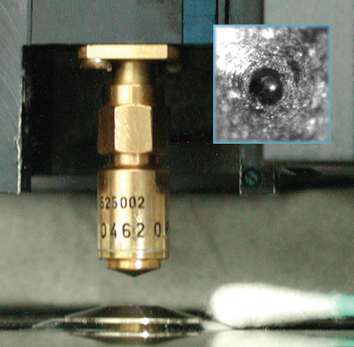
The nonreflected part penetrates the solid where it further propagates as a longitudinal wave. Excitation of the boundary surface causes it to move up and down, and this oscillation propagates as a transversal surface wave. At a specific angle of incidence (the Rayleigh angle), the whole impinging acoustic wave may move along the surface of a surface, being split into a longitudinal and a transversal surface wave, both propagating with the same phase velocity and finally leaking back to the lens. These waves are called Rayleigh waves or leaky surface waves. Interference of Rayleigh waves with waves reflected from the surface of a probe is the basis of V(z) characteristics (Fig. 12.1).

Figure 12.1 Acoustic broadband lens (gigahertz range) mounted on an ELSAM® microscope scanner and adjusted to a light microscope (lens is facing an objective lens of the light microscope). Inset: Top view of the acoustic lens with the spherical cavity in the middle. This cavity, with about 30 μm diameter, focuses the ultrasound. The broad surface around this cavity is roughened to decrease internal lens reflections. Photo by C. Blase.

In fluids or soft materials (as in biological tissues), no surface waves are induced, or they will be strongly attenuated.

Contrary to electromagnetic wave spectra, no transparency window exists for acoustic waves. They become monotonically attenuated, increasing with the square of frequency. Attenuation at a given frequency is defined by the decrease of amplitude of a wave depending on the distance (x) passed:

12.5

where α_I is the attenuation coefficient related to intensity decrease and is measured in Neper (Np) or in Bel. Normally, it is given as 1/10 of a Bel (dB) corresponding to

12.6

where I₀ and I are the sound intensities at the beginning and end of the distance, respectively.

12.1.2 Main Applications of Acoustic Microscopy

Because acoustic-wave-based images reveal mechanical parameters only, no staining is required to produce contrast in the case of tissue sections or isolated cells. This consideration was the motivation of Lemons and Quate (1974) for the development of a Scanning Acoustic Microscope (SAM) in the early 1970s. Whether this anticipation will hold true remains doubtful after the very slow increase in biomedical applications. Until now, most of the applications have been found in materials sciences, where, for example, delaminations of thin layers or microcracks can be detected with extreme sensitivity.

In the biomedical field, the main studies have been on tissue sections of the cardiovascular system, skin, and intestine, as well as investigations on the mechanical properties of bone and cartilage. In addition, cells in culture were the favourite specimens of the author and a few others. Many of the previous difficulties in image analysis have been overcome during the past years, and diagnostic as well as therapeutic sonography experienced a huge advancement.

A first comprehensive review on theory and applications was edited by Andrew Briggs in 1992 and continued in further issues in 1995. More recently, an updated view on theory and applications in material sciences as well as in biology and medicine has been edited by Kundu (2004).

12.1.3 Parameters to Be Determined and General Introduction into Microscopy with Ultrasound

The main parameters of biological tissues revealed by acoustic microscopy are geometry (thickness), mass, and elasticity, which taken together are related to the speed of the sound waves within the materials and structural organization represented by sound attenuation. Depending on the frequency used, the lateral resolution is in the range of a light microscope (around 1 μm at 1 GHz); under specific conditions (e.g., at liquid He temperatures), frequencies up to 8–10 GHz can be reached, corresponding to resolutions close to 100 nm (Foster and Rugar, 1983, 1985). A resolution of 10–20 nm in the vertical axis of an acoustic lens is easily achieved if interference phenomena are evaluated. Very high intensities within the focal spot can give rise to nonlinear phenomena by multiple phonon reactions and, by this, considerably increase resolution (Foster and Rugar, 1985). In general, a strict determination of lateral resolution is not possible; it strongly depends on the transfer characteristics of the acoustic lens, the contrast, and the wavelength. Experimentally it is best determined by calculating the spatial frequencies from the Fourier spectrum of a line scan of a specimen containing high spatial frequencies (Block et al., 1990). Commercial instruments are operated up to a maximum of 2 GHz. The lower frequency limit is more difficult to define; in most cases, it will be considered around 100 MHz. Sound waves of this frequency are strongly attenuated in air; therefore, the transducer has to be coupled to the specimen via a fluid layer. Attenuation of waves within this coupling fluid layer represents the main limit for using high frequencies; another limiting factor is lens design for high frequency imaging.

The idea of using ultrasound for microscopic imaging dates back to Sokolov (1949) who first viewed ultrasound waves projected via a lens on the surface of water. Most acoustic microscopes used are SAMs. One of the goals envisaged by investigators performing acoustic microscopy is a better understanding of the parameters controlling diagnostic sonography. Another source of interest is the increasing acceptance of mechanical forces as mediators in embryonic development (Beloussov, 1998; Beloussov et al., 1994), cell migration (i.e., in wound healing, invasiveness of cancer cells or embryonic foldings), cellular differentiation (e.g., Emerman and Pitelka, 1977; Kippenberger et al., 2000; Lyall and El Haj, 1994), and health impairments by pathological changes of tissue mechanical properties as in atherosclerosis (e.g., Saijo, 2004; Saijo et al., 2001) or osteoporosis (eg. Maia et al., 2002; Paschalis et al., 2004). Combined with specific contrast techniques (gold or nanobubble coupling of target molecules), acoustic microscopy will be extended to the molecular level (van Wamel et al., 2006). This, however, remains to be studied in future experiments. Therapeutic applications of ultrasound have not been performed on the microscopic level, although ultrasound in the lower megahertz region can be used for local membrane permeabilization (sonoporation) as required, for example, in cell transfection (Bao et al., 1997; Frenkel et al., 2002; van Wamel et al., 2006) and a variety of therapeutic approaches as in tumor treatment (Liu et al., 2005) and drug delivery (Bekeredjian et al., 2005). Tumor cell killing very much depends on the type of tumor and seems to be based on cellular membrane disruption, including plasma membrane as well as mitochondrial membranes, and therefore require quite high energy densities, that is, 3–4 W cm⁻² for 60 s at 2.2 MHz (Wang et al., 2009). At even higher intensities reached by focusing ultrasound on the muscle of mice that were fully alive (800–300 W cm⁻² at 1 MHz for 20 s four times with 2 weeks interval and spot size of 1.5 mm), expression of Cytomegalovirus (CMV)-promoted luciferase expression in transfected mouse muscle had been stimulated up to 6.5 fold (Hundt et al., 2009). Thus, the reaction of different tissues to ultrasound cannot be predicted at the moment.

12.2 Types of Acoustic Microscopy

In principle, transmission and reflection techniques have been developed. For transmission systems, see, for instance, Ashman and Rho (1990), Kulik et al., (1992), and Maev and Levin (1997). From the very beginning, acoustic microscopes have been combined with other imaging techniques, that is, confocal laser scanning microscopy, fluorescence microscopy (Blase and Bereiter-Hahn, 2004; Kanngiesser and Anliker, 1991; Lüers et al., 1992; Lemor et al., 2004; Rabe et al., 2002) with microinterferometry (Bereiter-Hahn, 1987b) or with scanning force microscopy (Kopycinska-Müller et al., 2004). Scanning acoustic microscopy operated in the reflection mode became the most widely used principle since its introduction by Lemons and Quate (1974), because it was provided commercially, for example, by Olmypus, Leica (now SAM Tec), and Honda Electronics. Therefore, I will concentrate on this type of microscopes, the evaluation procedures, and some of the results achieved. In addition, the combination of a light microscope with an ultrasound transducer unit to observe ultrasound-induced oscillations of microbubbles (or cells in suspension), which was constructed by Postema at the Erasmus Medical Center in Rotterdam (Postema et al., 2004), will not be included.

12.2.1 Scanning Laser Acoustic Microscope (LSAM)

The general setup of this type of microscope was the first type of acoustic microscope brought to work (Korpel et al., 1971). The Laser Scanning Acoustic Microscope (LSAM; Kessler, 1976; Rudd et al., 1987) combines interaction of a specimen with plane ultrasound waves (typically 100 MHz) and a readout via scanning laser interferometry, revealing its shifts in phase and amplitude of the deformation of a thin gold layer, which acts as a receiver of the sound waves after passing the specimen. This principle has been used widely for the investigation of tissue sections (e.g., Agemura and O'Brien, 1990). Because this is a transmission-based microscopy and flat specimens are investigated, some of the interpretation problems that are due to varying slopes of reflecting surfaces are avoided, and therefore, attenuation and elasticity values are very well presented by this method.

12.2.2 Pulse-Echo Mode: Reflection-Based Acoustic Microscopy

These microscopes are all SAMs of the confocal type. Thus, the images are derived from point-by-point scanning of a specimen and represent data obtained for each pixel in a 2D matrix. The confocality and selection of a narrow time gate for the reflected pulse include the possibility of 3D imaging, which, however, was not very widely used in the past. Three-dimensional images have been calculated from thickness measurements (Fig. 12.12), but this is not real 3D imaging. More recently, real 3D images are reconstructed from time-resolved SAM.

In the very heart of such a microscope is the acoustic lens, which in the case of frequencies >100 MHz typically consists of a cylindrical sapphire with a plane side bearing the transducer element and a small spherical cavity on the opposite side directed toward the specimen (Figs 12.1 and 12.2). For gigahertz lenses, the cavity diameter is in the range of 30 μm within an area of about 5-mm diameter and has a roughened surface to reduce sound reflections within the lens. The velocity of sound is about 11.100 m s⁻¹ in sapphire and 1500 m s⁻¹ in water (used as a coupling fluid); thus, the refractive index ratio amounts to 7.5 compared to 1.5 in light microscopy. Chromatic dispersion, therefore, is low, but losses at the lens/water interface due to reflections are a severe problem, which is overcome only in part by surface coatings. The influence of lens and electronic device on image generation has been discussed in detail by the group of Boseck (Block et al., 1990).

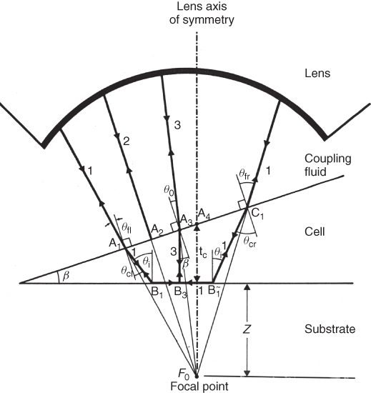
Figure 12.2 Scheme of an acoustic lens and course of sound waves interacting with a cell (oblique surface) on a solid substrate. The spherical cavity at the site where the lens is coupled to the object via a sound-propagating fluid renders the plane wave to converge in a focal spot. For ray 1, diffraction at the coupling fluid/cell interface (at A1) and then the formation of a Rayleigh wave from B1 to B1 is shown. With ray 2, sound reflection from the cell surface is exemplified, and ray 3 describes the reflection from the substrate. The focal spot in this case lies within the solid substrate. Angles θ mark the changes in the direction of sound propagation by diffraction. Source: From Kundu et al., 1991.

The transducer is a piezoelectronic actuator (a thin ZnO film), with its crystal axis perpendicular to the surface of the sapphire, which becomes activated by oscillating voltage and thus contracts and dilates periodically with the frequency of the oscillating voltage. By this, a plane wave is generated within the lens material, propagating along its length. The spherical cavity at the site where the lens is coupled to the object via a sound-propagating fluid renders the plane wave to converge in a focal spot (Fig. 12.2). Its size depends on the aperture of the acoustic lens, that is, the diameter of the cavity and focal length. As in every confocal method, the size of the focal spot determines the spatial resolution of the microscope. For 100 MHz, the resolution limit is about 15 μm, with a penetration depth of 4 mm; at 2 GHz, resolution is 0.75 μm (or better), but penetration depth decreases to 10 μm.

In the reflection mode, the same lens that sends the acoustic pulse (typically 4–25 ns long) acts as a receiver; however, two lenses may be used arranged in opposite positions, one sending the sound wave and the other focused to the same plane acting as a receiver. Most of the commercial instruments (Fig. 12.3) are operated in the reflection mode; therefore, only this type is discussed. In these cases, a fast circulator switches between the oscillating frequency inducing the ultrasound and the amplifier chain processing the signal produced by transforming the reflected sound wave into a voltage oscillation. This is superimposed on a carrier frequency, and after amplification within a heterodyne amplifier, it may be visualized on a screen or digitized and stored as a digital image. Considerable diversification of instrumental details occurred within 20 years of the introduction of commercial instruments.

Figure 12.3 Two acoustic microscopes that are distributed by PVA Tepla (Westhausen, Germany). (a) High resolution instrument “Evolution PII” (f ≤ 2 GHz) with integrated light microscope. In this image, the head with the acoustic scanner is moved toward the left. (b) Instrument of the Evolution-series (Evolution II) in the frequency range between 3 and 400 MHz with large motorized scan width for samples up to 520 mm × 380 mm × 45 mm (w/l/h) and water tank for the specimen. (Images courtesy of PVA Tepla, Westhausen, Germany).

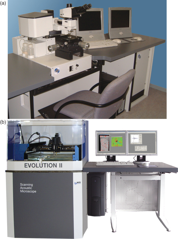
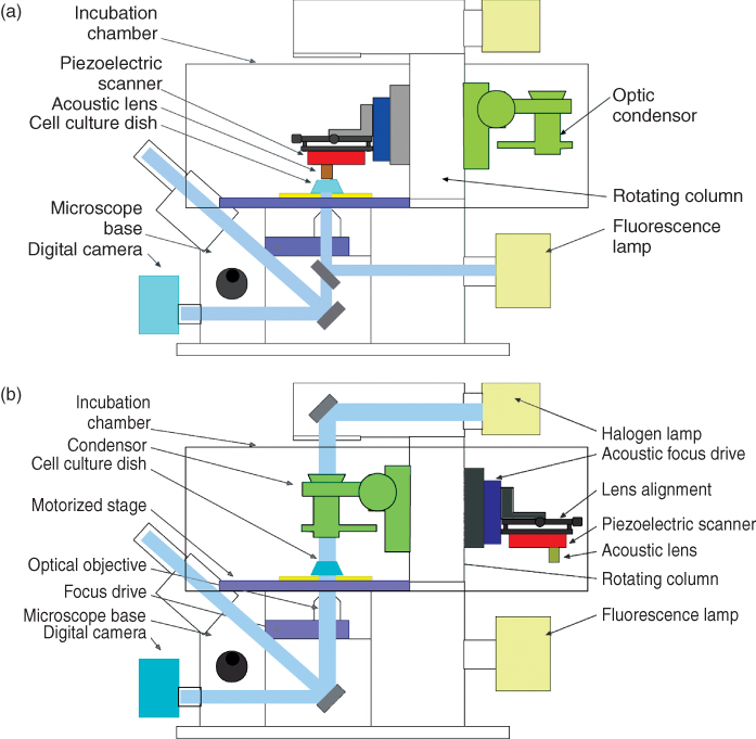
Figure 12.4 Schematic drawings of the SASAM system, an acoustic head integrated into an inverted fluorescence microscope, produced by the Institut für Biomedizinische Technik (St. Ingbert). (a) Acoustic head in active position (above the specimen). (b) Transmitting light condensor in active position, acoustic head turned to opposite side. Drawings courtesy of E.C. Weiss and R. Lemor.

Many of these modifications are laboratory prototypes and can be used only by personal collaboration; the development of commercial instruments was impaired by a relatively low number of instruments sold. The main advantage of the more recent developments is in the signal stored. The early high resolution instruments working in the gigahertz range, such as the ELSAM from Leica (Wetzlar) and the high frequency operated Evolution PII from PVA Tepla/KSI (Herborn and Westhausen, Germany), use the amplitude of the reflected sound signal received within a certain adjustable time window for image generation, which then might be digitized (32 bit in the case of the PII SAM). The “Evolution PII” instrument, for instance, sets time gates with a width down to 2 ns. In some recent brands working between 50 and 300 MHz (e.g., HMC by Honda Electronics, Toyohashi) or at about 900 MHz (SASAM from IBMT, St. Ingbert, Lemor et al., (2004)), the whole reflected signal along a series of meandering scanning lines (C-scan, including the B-scan for each pixel) is collected and may later on be processed to produce images either by using an amplitude overall image or by filtering certain time gates representing, for example, surface reflections only from a specimen or separating the reflections from a solid surface bearing the biological material from other reflections and thus allowing for the determination of attenuation. At gigahertz sound frequencies, full signal collection represents a high technical challenge.

The main features of instruments determining their practical use are as follows.

12.2.2.1 Reflected Amplitude Measurements

Measuring sound reflected at the interface between coupling fluid and specimen (I_r/I₀) allows straightforward calculation of impedance (Z_S) and sound velocity (c_S) of a specimen using Eq. 12.2 or 12.4.

Sound velocity (c) in a body is a function of the appropriate elasticity modulus. In fluids, this is primarily the compression modulus (K):

12.7

where G is the shear modulus and ρ is the density of the liquid in grams per cubic centimeter. Commonly G K; therefore, Eq. 12.8 is approximated to

12.8

The relationship between the elastic modulus, E, and the compression modulus, K, is given by

12.9

where μ is the Poisson ratio (e.g., for actin filaments about 0.4; Ziemann et al., 1994). The elastic modulus, E, is then 0.6 times the compression modulus, K.

Surface reflectivity has been widely used in a broad range of frequencies for the determination of elastic properties of biological hard tissues such as bone, dentin, or enamel (e.g., Maev et al., 2002; Meunier et al., 1988; Peck and Briggs, 1987; Raum et al., 2003a).

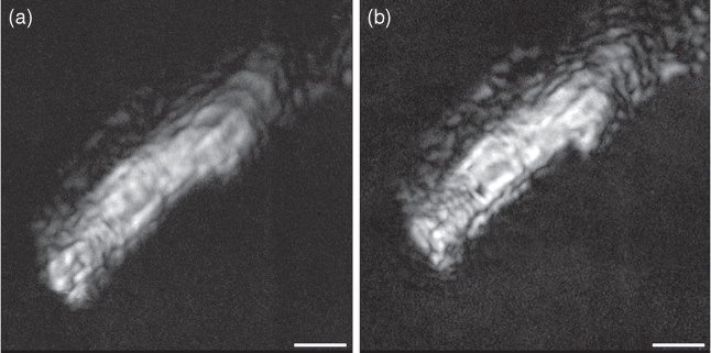
An example for measurements with this method is given: an “allmax” projection of a set of acoustic images taken from an isolated rat cardiomyocyte (Fig. 12.5). Adult cardiomyocytes are a good example for a specimen well suited for analysis by sound reflection measurements, but it also shows the limitations of this method. Because of cell thickness, reflections from the plastic material of low impedance supporting the cell do not interfere with the measurements. Separation of reflections from different surfaces can be improved by setting a narrow time gate for the reflected signal used to image a specimen. This is available for most of the commercially available instruments. From a single image, no distinction can be made between local differences in reflectivity caused by impedance differences or by the slope of the surface. This would require monitoring the phase of the reflected sound (which would shift with local thickness variations) or focus series. This was done by taking a series of images with a 0.5-μm increment in focal position; then, the brightest value for each pixel position (x_i, y_i) found in the whole set of about 20 images was written into a new image, thus showing only the brightest reflections at each point (“allmax image”). The focus increment has to be smaller than the focal depth of the acoustic lens to fulfill the Nyquist sampling theorem. In the case of 1 GHz, vertical resolution of the amplitude image is in the range of 3 μm; therefore, a recommended step size of 0.5 μm corresponds to sixfold oversampling. A detailed description of the physics of image reconstruction from such series has been provided by Raum et al., (2003a).

Figure 12.5 An “allmax” projection of a set of acoustic images taken from an isolated rat cardiomyocyte in relaxed (a) and contracted (b) state. Bar: 10 μm (courtesy of Dr M. Riehle).

Additional limitations of this method are represented by the anisotropic structure of the probe. Only sections will allow for determination of acoustic anisotropy.

The simple relationship described by Eq. (12.2) is valid only for normal incidence. The assumption of normal incidence of ultrasound focused on a plane surface is justified in the focal plane because of the specific propagation pattern in the focal spot of an acoustic lens. If the focal plane of a lens is positioned several wavelengths above the surface to be imaged, only normally incident sound waves contribute to image formation. In many cases, the slope of the reflecting surface is not exactly known; therefore, the extended formula (including this obliqueness) cannot be applied, and thus only those parts of specimens that lie at approximately 90^° to the incident sound beam can be studied. Examples of almost plane surfaces are tissue sections and very flat cells in culture (reflectivity does not change more than 5% if the slope of the reflecting surface of a cell is up to 15^° (Weise et al., 1994)).

12.2.2.2 V(z) Imaging

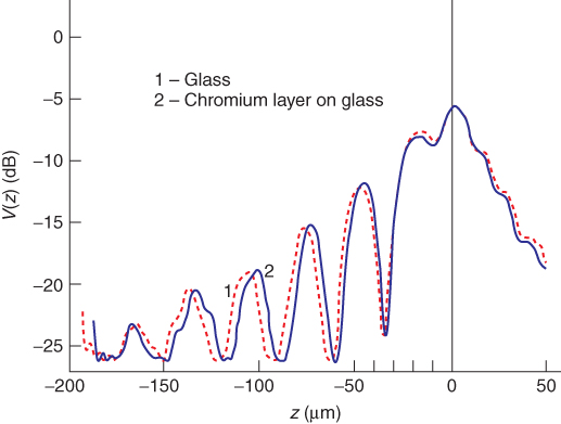
A special case of reflection mode scanning is V(z) scanning (voltage vs focus position). While focusing beyond the surface, because of interference between the acoustic waves reflected from the surface and the Rayleigh wave emitted back to the lens, periodic changes in reflected amplitude occur, which are characteristic for each material (Fig. 12.6). This method can well be applied to biological hard materials (e.g., Block et al., 1990; Raum et al., 2006). The reflected voltage (V) in relation to focus position (z), as shown in Figure 12.6, is given by

12.10

where U is the sound field produced by the transducer, P is the pupil function of the acoustic lens, R is the reflection function of the specimen, r is the radial position of the signal in the back focal plane of the lens, f is the focal length of the lens, r/f is the sinus of the aperture angle of the lens in combination with the coupling fluid, α is the half aperture angle of the lens, and k₀ is the wave number in the coupling fluid.

Figure 12.6 V(z) curve for glass and glass covered with a 200-nm thick chromium layer (broken line) taken at 200 MHz (with an Olympus UH2 microscope). This curve has been obtained by plotting the reflected signal while focussing from the focus position on the glass surface (0—position) into the glass (negative focus positions) or above this surface (positive focus position). The thin chromium layer modulates the V(z) signal. These modulations can be used to determine the acoustic properties of any superimposed layer with unknown properties. (From Block et al. 1990, with permission).

Although Rayleigh waves are missing within soft biological material, this material shifts the maxima and minima of the Rayleigh spectrum because sound velocity in the sample differs from that in the environment.

Modulations of hard material V(z) curves by thin layers of soft material can also be used to calculate the acoustic properties of a thin layer of biological material. The theory of this model has been developed independently by several groups (Block et al., 1990; Chubachi et al., 1991; Kundu et al., 1991; Litniewski and Bereiter-Hahn, 1992; Yu and Boseck, 1992). Using a small part of V(z) characteristics, allowed for the first time, mapping of elasticity (sound velocity) and attenuation over a cell with full resolution of the SAM (Bereiter-Hahn et al., 1992) (Fig. 12.13). More recently, Raum et al., (2003b) used the full Rayleigh spectrum obtained by large defocusing. Kundu et al., (1991) modeled cell properties from small defocusing only. The advantage of large defocus is the unambiguity of the calculations, which has to be introduced by setting limits in the calculations with the simplex approach used for small defocus images. The latter method was chosen because, for living cells, data acquisition time has to be as short as possible to avoid changes in cell parameters while the images are taken. Such active movements may be enhanced by fluid perturbation over the very small distance between the scanning lens and the cell surface: approaching the moving lens even more toward the cell increases the influence of fluid mechanics on the cell surface and supposedly evokes physiological reactions, thus obscuring the “real” situation. However, this influence has never been investigated systematically. For the investigation of tissue sections, large-range V(z) analysis is a very elegant and reliable method.

The main advantages of this method are that it is a well developed theory, it is widely used in materials sciences, it offers high lateral resolution, and thin cytoplasmic layers can be analyzed. All the parameters can be calculated separately only in the microrange V(z); bounds for the values are required to allow the simplex algorithm to converge to the correct set of values. A broad variety of substrata can be used to mount the specimen, and no interferences are required for the calculations.

The main disadvantages are the long acquisition time (several images are required) and the dependence on substrate properties, which must give distinct V(z) curves.

12.2.2.3 V(f) Imaging

Variation of frequency has been used in light interference microscopy for the determination of two unknowns: thickness and refractive index (Bereiter-Hahn et al., 1979). A similar procedure can be applied in SAM (Kundu et al., 2000, 2006 and others). Using a phase- and amplitude-sensitive modulation of a SAM (Hillmann et al., 1994), longitudinal wave speed and attenuation in a cell or tissue section, as well as thickness profile are obtained from the voltage versus frequency or V(f) curves. The challenge to determine at least four unknown parameters (speed of sound, attenuation, specimen thickness, and density) from acoustic images requires at least five images for reliable calculations. Grabbing a series of pictures in the range from 980 to 1100 MHz, with an increment of 20 MHz, allows the experimental generation of V(f) curves for each pixel by simply changing the signal frequency while keeping the lens–specimen distance unchanged. Both amplitude and phase values of the V(f) curves are used for obtaining cell properties and the cell thickness profile. Cell thickness, longitudinal wave speed, and attenuation can be estimated from the phase and amplitude for each pixel by the simplex inversion algorithm in a manner similar to V(z) analysis. Theoretical analysis shows that the thin liquid layer, between the cell and the substrate, has a strong effect on the reflection coefficient and should not be ignored during the analysis (Kundu et al., 1991).

The main advantage of this method is that imaging can be done near the focal plane. Therefore, an optimal signal to noise ratio is achieved, no interference with Rayleigh waves occurs, and the method is independent from the properties of the solid substratum where the cells are growing on. This method allowed us to monitor by SAM the reaction of cells to mechanical stretch (Karl and Bereiter-Hahn, 1998). However, this method requires appropriate broadband lenses, which still cannot be produced reproducibly with the desired properties.

12.2.2.4 Interference-Fringe-Based Image Analysis

Thin layers of biological material on the supporting glass or plastic surfaces may give rise to interference of reflections from the surface of the sample with those from the supporting material. Prerequisites for such interferences are a sufficiently long sound pulse, small thickness of the sample (“small” relates to wavelength of sound, <6–8λ), and almost parallel reflecting surfaces (slope <15–20^°). Cells in culture exhibit an oblique surface relative to the supporting glass or plastic surface. Therefore, reflections from the substratum and from the surface of the biological sample cause a series of concentric interference fringes (Figs 12.8 and 12.9). These provide a useful signal for a fast and orienting analysis of shape, elasticity, and attenuation of the cells. The contrast of the interferences depends on the impedance of the solid material bearing the cells. Materials with high impedance, such as tungsten layers on glass or glass itself, give rise to very strong reflections that are only slightly modulated by the weak reflections from the surface of the cells; thus, the images are dominated by attenuation, while plastic materials have lower impedance and therefore interference fringes exhibit higher contrast. From the sum of adjacent bright and dark peak values, attenuation by the specimen can be calculated, while the difference of those values allows to calculate sound velocity (for detailed description of the method, see Litniewski and Bereiter-Hahn, 1990).

Figure 12.7 Schematic drawing of the cross section of a cell (blue, cytoplasm; yellow, nucleus) interacting with sound. The sound wave emitted from the acoustic lens (black ray) is partly reflected from the cell surface (blue line) and partly penetrates the cell to the solid substratum (e.g., plastic material or glass), where a fraction is reflected according to the acoustic impedance of the solid. Both these reflections interfere with each other, yielding a cell picture as exemplified for a group of HaCaT cells shown in Figure 12.8. (image width, 200 μm). (Courtesy of Dr. C. Blasé).

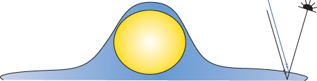
Figure 12.8 HaCaT cells on plastic as viewed by 1GHz acoustic microscopy (ELSAM). The course of the interference fringes indicates surface topography. Where the cells are not in contact with neighbors the develop a broad flat cytoplasmic layer (very broad interference fringes). The bright spots in the central cell indicate zones lacking contact to the plastic surface.

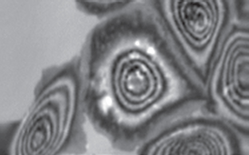
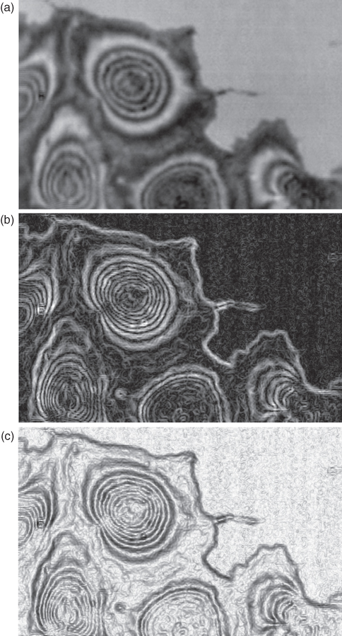
Figure 12.9 Example for visualization of the contrast function in an acoustic image by Sobel filtering. (a) The original SAM image of a group of HaCaT grown on a plastic culture dish, 1 GHz. (b) The first derivation of the original picture representing the intensity changes within the picture (Sobel filtering). To facilitate interpretation of this image, it will be inverted and thus results in (c). High contrast in the original is revealed by the black appearance, low contrast by brighter or gray areas. In addition, very fine structures become visible.

The approximate cell shape (topography) is immediately obvious from the pattern of interference fringes seen in SAM images. When applied to cells growing on a flat, solid substratum, these interference fringes delineate zones of equal acoustical path lengths between the reflecting boundaries, cell/culture medium and cell/substratum. Local variations in V_c would shift the position of an interference fringe; therefore, their pattern is only a first approximation to surface topography.

The big advantage of this method is its speed: a single amplitude image (scanning time <5 s) of a specimen is sufficient to calculate sound velocity, giving an estimation of elasticity. However, the method has several shortcomings: lateral resolution is limited to the distance between adjacent maxima and minima of interferences, and mechanical properties are assumed to be constant over this space. Reliable measurements require a solid substratum with relatively high impedance, that is, glass, and thus the overall contrast of these images is low, and the distance between lens and specimen is about 8λ apart to reach normal incidence, thus intensity is low. The procedure is limited to those areas showing interferences, and the order of interferences must be estimated properly. The density of the cytoplasm is assumed to be constant at an estimated level.

Therefore, this method was primarily used to follow dynamic events. The local dynamics of elasticity are easily visualized by Sobel filtering of the primary images taken at z-values a few wavelengths above the specimen. Sobel filtering reveals the steepness of gray level changes in between constructive and destructive interferences and thereby visualizes contrast (Fig. 12.9). Thus, as a first approximation, this filtering can be used to show elasticity distribution and is well suited for comparative observations of force distributions in migrating cells (Bereiter-Hahn and Lüers, 1998).

Contribution of substrate reflections can be avoided or at least strongly reduced by using substrates with an impedance close to that of the specimen under investigation or if the investigated specimen is thick, by sufficiently large defocusing. Materials almost matching cytoplasmic impedance are concentrated agar (>3%) or soft polyvinylchloride (Kanngiesser and Anliker, 1991).

12.2.2.5 Determination of Phase and the Complex Amplitude

Acoustic microscopy based on imaging phase and amplitude gives an easy access to all the data necessary for unequivocal evaluation of mechanical parameters of specimen in the reflected sound mode. For this purpose, an ELSAM has been equipped with an electronic circuit, allowing separation of the phase and the amplitude of the reflected signal (Fig. 12.10). The method has been presented in detail by Hillmann et al., (1994) and Grill et al., (1999). The probe-dependent phase shift of the signal can be achieved by comparing it with a reference derived from the sending oscillator. This multiplication is technically realized with a mixer followed by a lowpass filter. The complex amplitude has to be determined by splitting the reference and the probe wave path and extending the probe path by a quarter wavelength before it is mixed with the reference signal.

Figure 12.10 SAM images of an endothelial cell (XTH-2 cell) on plastic material taken at a series of different frequencies (here are shown 0.98 and 1.1 GHz). The phase change of the reflected sound and its intensity modulation by attenuation and interference phenomena are presented and then used to calculate the thickness and speed of sound along a chosen scan line, plotted in the graph. In this case, the presence of a thin layer of fluid between the cell and the solid substrate was assumed and incorporated into the calculations Source: From Kundu et al., 2000, with permission.

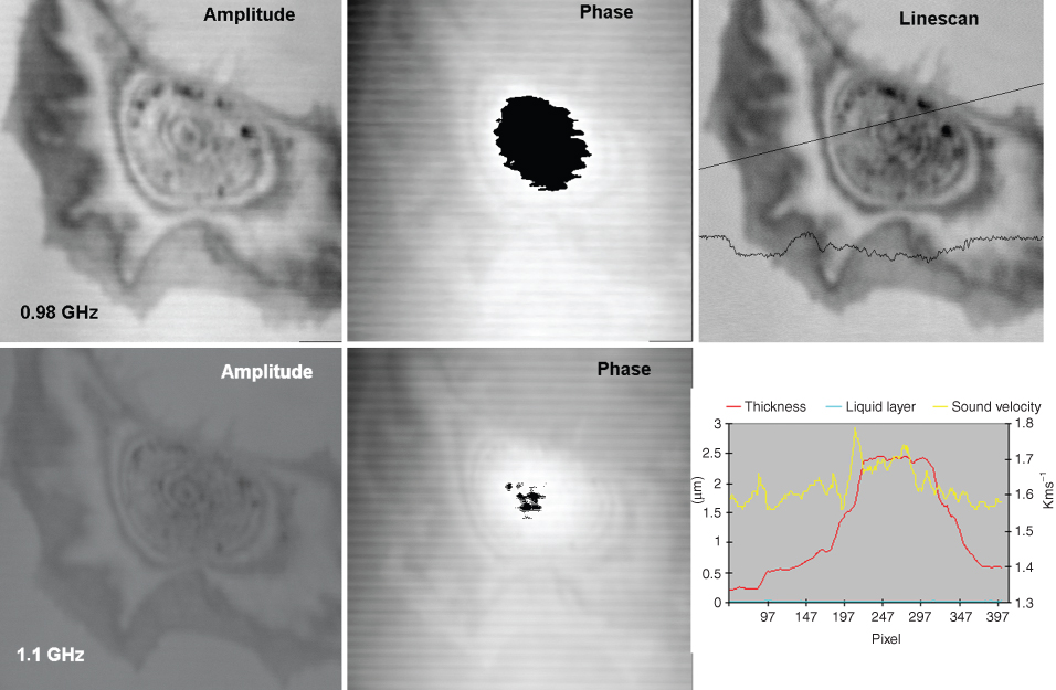
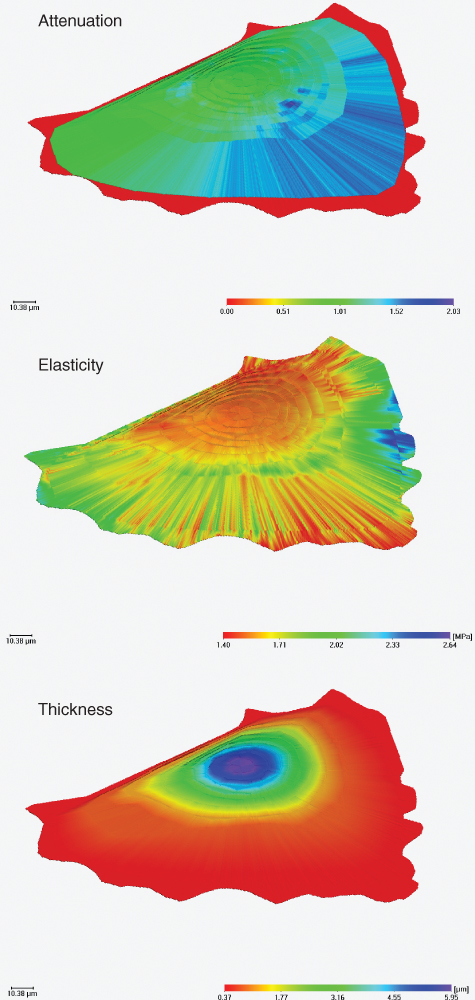
Figure 12.11 Reconstruction of the distribution of thickness, elasticity, and attenuation all over an endothelial cell (XTH-2 cell) in culture. This reconstruction is based on pictures taken at three different frequencies (from Hartmann, 2002).

12.2.2.6 Combining V(f) with Reflected Amplitude and Phase Imaging

Speed was the main advantage of the interference-based method for cell mechanical properties (Litniewski and Bereiter-Hahn, 1990). However, it allowed only rough estimations of impedance (speed of sound, i.e., elasticity) and attenuation, all these at lateral resolution defined by the distance of constructive and destructive interferences. Shifting interference fringes using different frequencies can fill the gap of low spatial resolution. Frequency shifts can easily be programmed, and thus a few images can be sufficient to fill all the gaps between the maxima and minima of the interferences. In addition, combining phase and amplitude information provides an easy means to precisely calculate sound velocity and attenuation.

The acoustic path length is unequivocally determined at any maximum or minimum of an interference fringe: it represents a multiple of the wavelength λ. Because in the reflection mode sound passes twice through a specimen, destructive interferences (dark rings) occur at a multiple of λ/4, while constructive interferences represent multiples of λ/2. The multiple is given by the order (m) of the interference. Because λ results from c/f, and frequency f is known, λ can be replaced by the sound velocity c and frequency f:

12.11

in the case of destructive interferences, and

12.12

in the case of constructive interferences.

From the phase image, ΔΦ (the phase difference between the sound waves reflected from an area devoid of specimen and the sound wave passing through a given volume of the specimen) can be defined by

12.13

from which the following equation may be obtained:

12.14

where c_f is the speed of sound in the coupling medium and c_c is the speed of sound within the cytoplasm. Young's modulus may be calculated according to Eq. (12.9). Attenuation is calculated from the sum of adjacent maximal and minimal amplitudes according to Litniewski and Bereiter-Hahn (1990).

If this procedure is performed for a single frequency only, 5 s of image acquisition (512 × 512 pixel) is sufficient with the Leica ELSAM, but the values have to be integrated for the spaces in between the extrema of the interference fringes. If pictures were taken at several frequencies (Δf in the range of 20 MHz at a basic frequency close to 1 GHz), the shifts of the fringes fill in the gaps left by the first image and thus spatial resolution increases up to covering all areas of a cell with the desired density of measurement points. Figure 12.11 gives an example of such a whole-cell reconstruction using three different frequencies, corresponding to 15 s image acquisition time.

12.2.2.7 Time-Resolved SAM and Full Signal Analysis

Time-resolved microscopy has been constructed independently several times in the past and has been used for characterization of soft and hard biological tissues (for review, see Briggs, 1992). The short temporal extent of the impulse excitation allows separate echo pulses from the top and bottom of a thin specimen or from separate interfaces in a layered specimen to be identified in the received signal, and hence the vertical structure in specimens can be resolved. High reflectivity of the supporting surface combined with low reflectivity of the specimens and attenuation by the samples normally impede this type of imaging soft biological samples. Cells grown on a polyvinylchloride surface, which almost matches the acoustical impedance of the coupling fluid (reflectivity 18 dB lower than the reflection of the surface of a polystyrene petri dish), were viewed using ultrasound pulses in the nanosecond range. This method permitted acoustical sectioning and thus 3D imaging and x/z scans (B-scans) with a resolution of 1.24 μm in the axial direction (0.54 μm lateral resolution at 1.5 GHz) (Kanngiesser and Anliker, 1991).

Analysis of time-resolved measurements does not require any a priori assumptions about the acoustic properties of the specimen and works well with tissue sections of about 10 μm thickness. Data from very thin cytoplasmic layers of cells in culture require extensive processing by the appropriate deconvolution algorithms.

Recent developments allow for storage of the whole course of a pulsed signal reflected from a specimen for all scanning positions at varying frequencies. Such systems are realized, for instance, by Honda Electronics, for the frequency range up to 200 MHz, step size of scanning is 4 μm constructing images of 480 × 480 pixels, and beam width is 5 μm at 200 MHz (Hozumi et al., 2004). This instrument has been extensively used by the group of Saijo for the analysis of cardiovascular tissues. This group considerably improved the acoustic system (Saijo et al., 2006): “The most important feature was use of a single pulse and the Fourier transform to calculate the sound speed at all measuring points. Although the data acquisition time of a frame was greater than that in conventional SAM, the total time required for calculation was significantly shorter that can measure the speed of sound of thin slices of biological material.” Deconvolution of the signal in the time domain enabled separation of the reflections from front and rear sides, and frequency domain analysis provided reliable data on sound speed in the range of 50–150 MHz (Saijo et al., 2006).

The “Evolution” series of SAM TEC (Westhausen Germany) shows the course of the signal in order to set a proper time gate to select the reflections from those distances containing the structures of interest. The mean amplitude of this selected part is stored and used for image generation.

The SASAM instrument provided by the group of. Lemor in the Institute for Biomedical Technology (St. Ingbert, Germany) reaches a much higher resolution by using about 1 GHz and saving the whole course of ultrasound signal for further calculations. The acoustic head can be coupled to any inverted light microscope (Fig. 12.4) and thus opens up the possibility of investigating simultaneously the very same area, for example, with fluorescence techniques, including confocal laser scanning microscopy and SAM (Fig. 12.12).

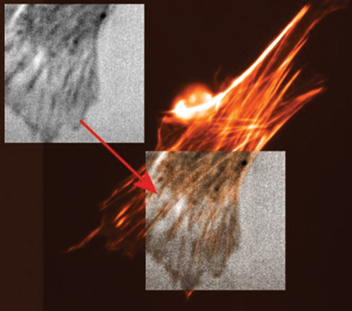
Figure 12.12 Coincidence of structures revealed by SAM imaging and fluorescence microscopy: embryonic chicken myoblasts were stained with Alexa-phalloidin (Molecular Probes: Eugene, Oregon) and the same positions were viewed with the SASAM and by fluorescence revealing F-actin. Focal contacts are represented as dark streaks in the acoustic image and can further be identified as the ends of stress fibers in the fluorescence image. The image size is 65 μm × 65 μm. (Courtesy of E. C. Weiss and R. Lemor, IBMT St. Ingbert).

12.3 Biomedical Applications of Acoustic Microscopy

12.3.1 Influence of Fixation on Acoustic Parameters of Cells and Tissues

Acoustic microscopy of biological samples does not depend on staining; fixation alone will be sufficient to reveal acoustic properties of cells and tissue sections (Hildebrand et al., 1981). Thus, the influence of freezing and thawing cycles—as required for freeze sectioning of organs—has been investigated qualitatively by Kessler, 1973; Parker, et al., 1984; and D'Astous and Foster, 1986; and quantitatively by van der Steen et al., (1991, 1992). This treatment does not significantly change acoustic parameters. Formalin fixation (4%, 1 week) of 5-mm liver cubes, on the other hand, has been found to leave speed of sound almost unaffected, while attenuation (at 5 MHz) increased it from 4.47 in fresh tissue to 4.96, paraffin embedding increased it to 11.62, and hematoxylin–eosin staining increased it to 16.01.

The first qualitative study on the influence of tissue fixation and processing on acoustic properties using 1.2 GHz transducer has been performed by van der Steen et al., (1992). They used 6-μm thick liver sections that were prepared in different ways: fixed either in ethanol or formalin; stained by hematoxylin–eosin, toluidin blue, or nonstained; cryostat sections or paraffin sections. Paraffin sections had to be deparaffinized to display any structure. Finer structures were displayed after ethanol fixation.

For cell cultures, fast air drying followed by rehydration in saline, Karnovsky fixation (mixture of glutaraldehyde and paraformaldehyde), and formalin fixation have been tested (Bereiter-Hahn et al., (1992)). Best preservation of morphology was reached by Karnovsky fixation; the acoustic parameters did not behave uniformly at 1–1.5 GHz showing many subcellular details. Least alterations were observed after air drying and rehydration. In general, attenuation was increased after fixation, in some cell areas up to fourfold as in the living state. Speed of sound decreased in the central cell areas and became more homogenous in the cell periphery. The interpretation was that local contractions no longer occur in dead cells. An example of fixation-related changes is given in Figure 12.13.

SAM investigations on soft tissue sections have been done on fixed or freeze-sectioned material. In paraffin sections, after deparaffinization, all the fat material of the tissue is removed, which is known to be of considerable influence on the acoustic properties of tissues (Brand et al., 2003; Sasaki et al., 2003). Thus, most researchers agree that freeze sectioning will influence acoustic parameters the least. Whether this represents elasticity in the organism remains an open question, because many tissues, for example, of the cardiovascular system, are under tension and this tension is released in the excised and sectioned material, thus the elasticity values measured are only elasticity values after full relaxation.

In hard tissues, the water content may be of more significant influence on the parameters to be measured than fixation (Currey et al., 1995). The influence of storage conditions on the elastic properties of dentin and enamel of human wisdom teeth has been investigated (Raum et al., 2006d), and it was revealed that artificial saliva was the fluid of choice for prolonged storage.

Calculating acoustic parameters of tissue sections has to deal with thickness variations as an additional factor of uncertainty (Okawai et al., (1988)).

12.3.2 Acoustic Microscopy of Cells in Culture

For isolated cells and soft tissue, calculations of impedance differences from the acoustic signal seems a relatively simple method to determine elasticity because the contribution of surface waves and Rayleigh waves can be neglected. Problems arise because reflectivity for ultrasound is low and, in addition to the elasticity of the cytoplasm or tissue structures, sound reflection may be modulated by surface topography, which depends on overall cell shape and presence of microstructures on top of the cells and at their surfaces adhering to a solid substratum (e.g., glycocalix, ridges, microvilli, microstructures exposed by sectioning of tissues). Several unknowns determine a SAM image of a cell or tissue: cytoplasmic elasticity, density, and, probably, viscosity have to be calculated from the acoustic parameters, sound velocity and attenuation, which are derived from sound reflections. These may be supplemented by measurements of time of flight and phase of the acoustic signal from which cell or section thickness (topography) can be derived. In the case of cells in culture, a thin layer of fluid in between the cell and the supporting substrate has to be considered because this layer may considerably influence SAM images (Bereiter-Hahn et al., (1992); Kundu et al., 1991).

How to cope with these unknowns? A variety of methods has been developed to solve this problem and to calculate physiologically relevant parameters from SAM images. The principles of the different approaches have been summarized above. In general, V(z) and V(f) procedures (V(z) and V(f) curves) require frequency or focus variations and need several images to be taken before the calculations can be done. This limits temporal resolution. Methods based on the evaluation of interference fringes provide high temporal resolution combined with loss in spatial resolution, and they do not allow measurements of very thin cytoplasmic layers because the maxima and minima of interferences are difficult to localize. Procedures taking advantage of the information in time, phase, and amplitude of the acoustical signal are superior. If all these parameters are collected, they require long time for image acquisition, extensive calculations, and space for data storage. All high resolution imaging methods are very sensitive to external disturbances (temperature, scanning plane, vibrations), which may impose difficulties for practical work.

Almost all the possibilities and shortcomings, the imaging and interpretation problems of SAM, can be demonstrated with live cell imaging; therefore, this application is discussed in detail according to the application of various methods to cell cultures that have been used in the author's and others' laboratories.

12.3.3 Technical Requirements

12.3.3.1 Mechanical Stability

SAM imaging is very vibration sensitive; therefore, the instruments are posed on vibration-reducing tables by the manufacturers.

12.3.3.2 Frequency

With increasing sound frequency and thus resolution, attenuation of the coupling fluid increases and thus the signal to noise ratio becomes worse. Heating to 37^°C reduces attenuation in relation to room temperature, and the required heating hood also stabilizes focus and thus is an indispensable tool for live cell investigation; also, in tissue section investigation, temperature must be kept stable.

12.3.3.3 Coupling Fluid

For biomedical investigations, saline is normally used as a coupling fluid. This gives optimal results because it has the least possible influence on the biological material, and the matching layer on the acoustic lens is optimized for sapphire/water interface. Sometimes methanol has been used as a coupling fluid, which also imbibes the probe. The advantage of using methanol is the lower sound velocity and thus smaller wavelength at a given frequency, which provides a chance for increasing spatial resolution; however, methanol itself changes the acoustic properties of the biological material and attenuates sound more than water, thus signal to noise ratio may become a limiting factor. This coupling fluid may be of help if frozen sections are going to be analyzed for morphological features without staining.

Protein-containing coupling fluids (cell culture media) may cause precipitations (probably of fibronectin) within the lens cavity and on the surface of cells, reducing the acoustic signal. Therefore, saline is preferable in all cases of investigation of tissues or cells.

12.3.3.4 Time of Image Acquisition

Scanning procedures produce sharp images even when the specimen is moving while the image is taken. So far, acquisition time does not seem to cause severe problems in SAM. However, mechanical properties of cells also underlie shape generation and motility, and these features can be studied only if the method of measurement (SAM) is fast in relation to the process to be analyzed (motility). Furthermore, all the analytic methods that require several images for calculation of the unknown cell parameters (e.g., V(z)- and V(f)-based SAM) have to start with the assumption that nothing changes during the time required for image acquisition, which was about 40 s for the V(z) series and has now been reduced to 25 s for a V(f) series. However, cells are dynamic as long as they are alive. As a consequence, fast moving cells (e.g., the speed of epidermal cells is up to 30 μm/min) cannot be analyzed at all by using V(z)- or V(f)-based evaluation methods. Cells that remain stationary on the scale of a few minutes might undergo shape changes. Therefore, we analyzed the overall cytoplasmic motility of nonlocomoting cells (i.e., keeping a constant position for at least several minutes) in culture. This is easily performed by subtraction of two subsequent images taken at a certain time interval (Fig. 12.14). By mathematical processing, the contrast of these different images can be improved. The differences were very small in most of the cultures; however, they led to the detection of clearly outlined domains of cytoplasmic motility (Vesely et al., 1994). These activities depended on cell density in those cultures that show contact-mediated control of locomotion and proliferation (Zoller et al., 1997). The motile activity measured by subtraction scanning acoustic microscopy (SubSAM) correlates well with the invasive potential of rat sarcoma cells and seems to be mediated by rac-activation (I. Karl and P. Vesely, personal communication).

Figure 12.13 XTH-2 endothelial cell before (a, b) and after (c,d) fixation: Using a small part of V(z) characteristics, for the first time allowed, mapping of elasticity (sound velocity: b,d) and attenuation (a,c) over a cell with full resolution of the SAM. Attenuation is increased after fixation and in the living cell represents areas with thick bundles of F-actin (arrowheads). Inverse behaviour of attenuation and sound velocity is seen in the two areas marked “1” in (b). The zone marked with the asterisk exhibits low attenuation and low elasticity as is typical for loose cytoskeletal networks often found in this area with the scanning electron microscope. 1 GHz, image width: 200 μm (from Bereiter-Hahn et al. (1992)).

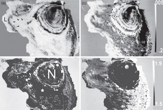
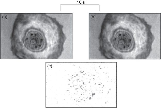
Figure 12.14 The method SubSAM is based on the subtraction of images gray level per pixel by gray level of the corresponding pixel in the second image. The absolute gray level differences were represented in the resulting subtraction image. The subtraction of images (a,b) taken from a living cell in a distinct time interval by scanning acoustic microscopy reveals domains, which represent the surface changes the cell undergoes in the meantime (c). Some of these domains represent ruffles (at the outermost cell margins); those in the more central parts of the cells just move up and down. The motility domains are related to receptor activations (compare Fig. 12.15), and cells differ in this behavior whether they are normal or tumor cells (from Karl and Bereiter-Hahn, (2001)).

Enhancement by selective receptor stimulation is in favor of the interpretation that these motility domains represent receptor fields (Fig. 12.15), probably membrane rafts. Because the motility domains become visible through the subtraction of interference images (sound waves reflected from the medium-facing surface interfere with those reflected from the substratum), surface topography changes down to about 15 nm are revealed and can be related to small local bulges also identified by light microscopic methods or by scanning electron microscopy.

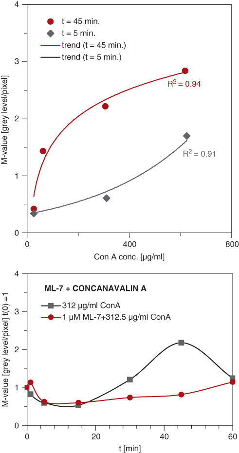
Figure 12.15 Quantitation of surface mobility as revealed by the procedure described in Figure 12.13. For reasons of comparability, an area-independent M-value was calculated on the basis of the gray level differences and the number of pixels in the SubSAM images. These M-values provide a measure of the surface mobility (Zoller et al., 1997). These curves give an example of stimulation of surface mobility by different concentrations of concanavalin A, its time dependence and its suppression by inhibition of myosin light chain kinase via ML-7 (lower panel). (From Karl and Bereiter-Hahn, 2001).

12.3.4 What Is Revealed by SAM: Interpretation of SAM Images

The primary parameters that can be achieved from SAM images are sound velocity and attenuation and thickness of the sample. According to Eqs 12.7 and 12.8, sound velocity is a measure of elasticity including density, but which elasticity is revealed, the one of the whole cytoplasm along the focus line or only that of the surface structures, is not known. Which of the cellular structures is primarily responsible for the elastic properties of a cell or tissue? What does attenuation mean in physiological terms? These questions are discussed in the present section.

12.3.4.1 Sound Velocity, Elasticity, and the Cytoskeleton

Mechanical properties of cells cannot be considered to be constant throughout the cytoplasm, neither laterally, that is, in the periphery and the center of a cell, nor along the acoustical axis, because the cytoskeletal and membrane arrangements in cortical cytoplasm layers often considerably differ from those in the central parts. Sound velocity derived from impedance changes at an interface, as, for instance, revealed by measuring surface reflection only is a measure of surface elasticity, while sound velocity revealed in a transmission mode measures the mean speed of sound throughout a specimen. V(z) and V(f) methods provide those mean values, while amplitudes of sound reflected from the surface of cells or tissue sections reveal impedance differences and thus the product of density and speed of sound. The structure responsible for the mechanical properties of the cell surface in fact is the fibrillar cortex (Fig. 12.16), which forms a mechanical unit with the membrane: actin fibrils are anchored to intrinsic membrane proteins. Changes in cortex tension will affect the activity of ion channels and influence the distribution of signaling molecules (i.e., receptors, adhesion molecules). Therefore, the mechanical properties of the cortex are of great importance for the control of a variety of cell activities, including proliferation activity (e.g., Ingber et al., 1995).

Figure 12.16 Optical section in x/y direction through a “fried-egg shaped” keratinocyte, and its cross section along the line indicated by the two marginal streaks in the x/y image. F-actin in this cell has been fluorochromed using TRITC–phalloidin. The cross section reveals the continuous F-actin layer beyond the cell membrane. Image by M. Voeth.

The next question is about the depth of the interface layer responsible for reflection. According to knowledge from light microscopy (i.e., total internal reflection techniques) this depth is restricted to a very thin layer of a few nanometers, much less than the extension of the focal spot along the acoustical axis. Thus, amplitude measurements of reflected sound, compared with amplitudes reflected from interfaces with known impedance differences reveal the speed of sound in the reflecting medium. Density of cytoplasm will be close to 1.06, and variations between 1.04 and 1.1 will not have considerable influence on acoustic impedance, which thus measures sound velocity. This is done in all cases where surface reflections are clearly separated from any signals of underlying material. Equations 12.8 and 12.9 can be used to calculate elasticity, but this term needs further consideration.

Cellular elasticity depends highly on the strain rate; in slow deformation processes viscous creep may become prominent (e.g., Hiramoto, 1986). In SAM, one can assume an extremely high strain rate (megahertz to gigahertz) together with an extremely small deformation (in the subnanometer range), thus viscosity does not influence the measurement that exclusively shows elasticity.

Further interpretation requires some basic assumptions on the physical state of cytoplasm, whether it is treated as a viscoelastic fluid (the widely accepted model) or a quasi solid, fibrous (or porous) matrix filled with fluid. This approach guides the interpretation whether bulk modulus or Young's modulus determines the longitudinal sound velocity according to:

12.15

where c_c is the longitudinal sound velocity in the cytoplasm, E is the appropriate modulus of elasticity, and ρ is the density).

Physiological interpretation of data derived from SAM measurements requires some further considerations.

For calculation of these properties, which are independent of the volume fraction of the material involved, the basic sound speed in saline (c_s) has to be subtracted from the value determined for the whole cell (c) because it represents the compression modulus of the ubiquitous saline, while the speed exceeding this value must be due to constants other than water and ions, which then are responsible for a cell's mechanical properties. In the case of cells or tissues in an aqueous medium, the sound velocity derived for the sample includes the sound velocity of the aqueous medium and that of the proteinaceous content. The contribution of the aqueous phase can be considered to be a constant in most tissues and cells. The proteinaceous fraction is the one causing the variation in the mechanical properties. It can be evaluated only when an assumption is made on the volume fractions of the protein (p) and the fluid space (q) of a cell.

12.16

where p and q are a measure of the relative path a sound wave travels through a specimen.

The overall speed of sound determined for a cell (c) is presented by

12.17

Thus, the speed of sound of the protein fraction (c_p) amounts to

12.18

and

12.19

For living cells in culture, a relative dry mass of about 20% is reasonable according to interferometric determinations. The sound velocity of the fluid phase in a cell is about 1550 m s⁻¹ (at 30^°C); thus, in the case of a mean sound velocity of 1600 m s⁻¹, sound velocity of the protein fraction can be estimated to be 1800 m s⁻¹; in the rare cases when sound velocities of 1800 m s⁻¹ have been measured, that of the protein fraction would be 2800 m s⁻¹. These values are in the range of polycarbonates.

The next question is, whether we are measuring bulk modulus (compressibility) or Young's modulus. In the case of a fluid, the situation is clear; fluids only have shear and bulk elasticity. Although the incident sound beam has a small diameter (in the range of 1–1.5 μm in water at 1 GHz), lateral displacements of the volume units exposed to sound are effectively attenuated; therefore, sound propagation is determined by compressibility only. The same can be assumed for highly hydrated proteins. This does not exclude, however, that Young's modulus of protein filaments under tension is the factor determining sound propagation. Mechanical properties of cells and tissues highly depend on the tension of fibers. In the case of tissues, these are primarily elastin and collagen; in the case of living cells, F-actin; thus the Poisson ratio determined for these fibrillar elements opens the possibility of relating compressibility to its modulus of elasticity (Young's modulus). Ziemann et al., (1994) determined the Poisson ratio (ν) for actin to be 0.33. In this case, the numerical value of the bulk modulus equals that of Youngs modulus (Eq. 12.9).

Tension caused by contractions of the actomyosin system thus will primarily contribute to the elastic modulus, as revealed by sound velocity. This can be shown experimentally by a short treatment with cytochalasin D, which releases tension from the actin fibrillar network almost immediately (30–60 s) (Bereiter-Hahn, 1987a), or on the other hand, by treatment with colcemid, which evokes strong contractions (Kolodney and Elson, 1995) resulting in extremely high sound speeds (Karl and Bereiter-Hahn, 1998). In both cases, mass does not change; only the arrangement and interactions of the fibrillar elements is altered. Another approach to clarify the cellular components and processes responsible for cytoplasmic elasticity as revealed by SAM was an experiment using the Ca²⁺-selective ionophore ionomycin. Addition of this drug in the presence of Ca²⁺ ions (1–2 mM) causes calcium influx into the cytoplasm, thus activating actin–myosin interaction and causing disruption of microtubules. This contraction immediately raises sound velocity in a site-dependent manner, that is, different cell areas react to a different extent. Finally, the high internal calcium concentration leads to disassembly of all the cytoskeletal fibrils, and sound velocity decreases to a level below that of the untreated cell (Lüers et al., 1992). These interpretations are possible because the very same cells have been investigated by fluorescence microscopy after SAM images have been taken.

These experiments showed the significance of active processes, of contractions of the actomyosin system in particular. Because of the intimate interaction of the three cytoskeletal fiber types and their control by signaling pathways, the contribution of a single fiber type to the elastic properties has not been revealed unequivocally. Very short cytochalasin treatment is the most specific one, which causes an immediate reduction of sound reflectivity from the cell surface.

The contribution of active contraction processes to the elastic properties of cells implies that investigations of any dead—fixed—biological material does not reveal the real in vivo elastic properties. This is also valid for determining elasticity of tissues that are exposed to stresses in the body; all these stresses are missing after fixation and sectioning. This explains the big differences in sound velocity as determined in tissue sections and in living cells with intact cytoskeleton.

12.3.4.2 Attenuation

Attenuation is an important factor in ultrasound imaging because no window of transparency exists in materials for sound. Attenuation theoretically increases with the square of frequency; however, linear increase has been reported for several biological tissues. What does attenuation tell us? This is a difficult question to answer. Early findings on cirrhotic liver suggested that attenuation increases with the protein content (Okawai et al., 1988). First hints on the structural basis of ultrasound attenuation came from the ratio of dry mass and attenuation in the cell periphery and the cell center. In the periphery, a small increase in dry mass led to a much higher increase in attenuation than in the cell center (Bereiter-Hahn, 1987b). The attenuation coefficient can be regarded to represent viscosity and thermal relaxation. Experimental data with biogels show that the influence of viscosity on attenuation is small and does not correlate. Using an oscillatory rod rheometer we continuously measured viscosity increase, speed of sound, and attenuation of 1 GHz ultrasound during the polymerization of actin (Wagner et al., 1999, 2001). During the nucleation phase, attenuation slightly decreased when actin polymerization (this does not influence viscosity) started and increased considerably after polymerization was almost finished. After polymerization, entanglement and bundling of F-actin occurs, and only this process is reflected by attenuation increase. To prove the hypothesis that fibrillar cross-linking is the main determinant for attenuation, actin has been polymerized in the presence of the F-actin cross-linking protein α-actinin. In this case, attenuation increases much more, and in step with polymerization. Other cross-linking proteins evoke the same behavior, and the high attenuation of collagen bundles (e.g., Saijo et al., 1996) can thus be hypothesized to be based on the extensive cross-linking of the collagen fibers within the bundles. Contrary to these findings and interpretations, breaking intermolecular cross-links in collagen reduced the attenuation coefficient of articular cartilage at 100 MHz SLAM investigations (Agemura and O'Brien, 1990). Increase of attenuation by various chemical fixation procedures can also be attributed to extended cross-linking by the fixative itself and/or by freezing steady-state cross-linking. On the other hand, elastic fibers that have a chemical composition similar to that of collagen attenuate ultrasound less than the cellular components of tissues (Saijo et al., 1996). Thus, thermal relaxation can be considered the main determinant of the attenuation coefficient (α) corresponding to

12.20

where ν is the frequency of ultrasound; τ is thermal relaxation, that is, time required for a molecule to reach its ground position again after being displaced by a force, according to (1-1/e); and c is the velocity of sound.

This relaxation time finally is a measure of viscosity. However, the numerical value of viscosity strongly depends on the size of the probe, that is, in an entangled fibrillar net, all molecules that are small in relation to the pore size experience low resistance against movement, while large organelles may not move at all through such a net, and thus viscosity appears to be very high at this level of probe size.

12.3.4.3 Viewing Subcellular Structures

As pointed out earlier, lateral resolution of SAM operated in the 1- to 2-GHz range comes down to < 1 μm. This feature will be revealed only for organelles or structures that differ in their acoustic impedance from that of their environment. In living cells, most organelles may not provide interfaces to be detected because their impedance matches that of the cytoplasm, and only in the case of cell death phase separation takes place. Figure 12.17 shows such an example.

Figure 12.17 Culture of endothelial cells (XTH-2) exposed to TRITC-phalloidin, which does not penetrate living cells. Upper image: SAM, 1.5 GHz, cells on glass. Lower image: Fluorescence microscope image of the same area. In cells that show TRITC-phalloidin fluorescence, small “vesicular” structures are visible in the SAM image, while in the unstained, living cells, the cytoplasm is almost unstructured; only a few black granules show up because of impedance differences to the cytoplasm. Image width: 200 μm.

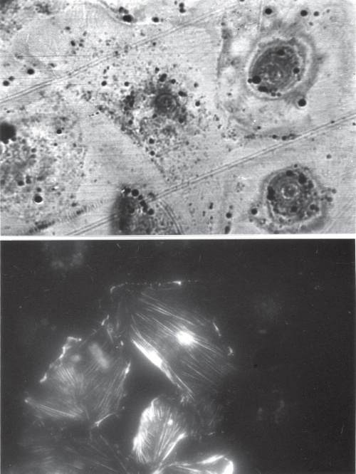
Figure 12.18 A group of HeLa cells was observed in the acoustic microscope SASAM. The numbers indicate the time of observation in minutes. At 150 min, the cell starts rounding and the nucleus is still visible; at 170 min, chromosomes are aligned in the equatorial plane and appear as a dark band; anaphase is going on at 180 min; at 190 min, the cleavage furrow is clearly visible; and cell spreading just starts at 220 min. At this time, the nucleus in the lower cell can be seen with its two nucleoli. Image size is 80 μm × 80 μm. This series has been taken by E.C. Weiss (St. Ingbert).

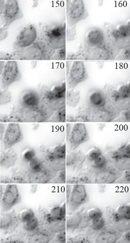
These cells have been exposed to tetramethyl-rhodamin-labeled phalloidin (TRITC-phalloidin). TRITC-phalloidin does not penetrate living cells; impaired or dead cells become permeable, and in these cells, the phalloidin strongly binds to F-actin. The fluorescence image and the acoustic image (taken at 1.5 GHz) show exactly the same field. Small granular substructures are revealed by SAM in the TRITC-phalloidin permeable cells, while the cytoplasm of the uninjured cells appears homogenous. This shows that although SAM resolution would be sufficient to reveal subcellular structures, they are hidden because of matching acoustic impedance. At this point, we should become aware that ultrasound at high frequency provides a nondestructive interaction with the biological material; the intensities are too small, and the attenuation is too high to allow for cavitation phenomena or for any living cell destruction. This, however, does not exclude that by stimulating surface receptors; biological effects other than cell death are evoked. We have made several long-term (up to 10 h) observations of living cells with an acoustic microscope, As an example the full process of mitosis in cell culture is shown in Figure 12.18, produced by the group of Lemor.

12.3.5 Conclusions

Acoustic microscopy provides unique possibilities for probing elastic properties of cells and tissues (for detailed introduction and review see Bereiter-Hahn et al., 1995; Briggs, (1992), (1995)). SAM has reached a state of development that allows routine investigations of biological samples (isolated cells, tissue sections, and tissue blocks). Specimens with large surface topographic variations may be reconstructed from focus series or from deconvolution of the reflected signal pixel by pixel. The maximum reflectivity at any point can be used to calculate local impedance and, thus, elasticity values. Evaluation of V(z) and V(f) provides a convenient key to subcellular distribution of elasticity and fibrillar interactions.

Cytoplasm and cellular organelles exhibit viscoelastic properties, that is, they are not adequately described as solid bodies or as fluids. In addition, cytoplasm and the organelles form microdomains that differ in their mechanical properties. A broad range of methods has been developed to determine viscosity (e.g., Hiramoto, (1986); Sackmann, (1997)); cytoplasmic elasticity, however, is more difficult to assess. Atomic force microscopy (e.g., Schoenenberger et al., (1997)) and the related poking methods are the most widely used principles to test cell elasticity. More recently, magnetic twisting cytometry added considerably to cytomechanical measurements and analysis of the physiological transduction of mechanical signals (Huang et al., 2005; Ingber et al., 1995).

12.4 Examples of Tissue Investigations using SAM

This section describes some results that have been achieved using ultrasound in the range above 100 MHz, thus of microscopy in a strict sense, with a lateral resolution approaching that of a light microscope. I do not intend to give a full overview on all the investigations performed but rather present a few basic findings that may encourage the reader to apply this technique to his/her own scientific problems.

12.4.1 Hard Tissues

Bone and cartilage are tissues with clear functions in biomechanics. They are a favorite object for sonographic and SAM investigations, because sonic investigation avoids the invasivity required for other types of biomechanical measurements. Early investigations on the microscope level were those of Meunier et al., (1988) and by high resolution by Hirsekorn et al., (1995). Turner et al., (1999) compared the Young's modulus of trabecular bone with that of cortical bone. The former was slightly higher than the transverse Young's modulus of cortical bone, but substantially lower than the longitudinal Young's modulus of cortical bone. More recently, the full range of frequencies between megahertz and 1 GHz have been applied for studying bone at different levels of resolution (Raum et al., 2003b, 2004). The challenge for all the applied experimental and mathematical models is to predict bone elasticity from structure, density, and mineralization. This relationship is by no means clear. Therefore, experimental data from SAM and other ultrasound-based studies have been compared with other types of mechanical and structural measurements, that is, microindentation (Bumrerraj and Katz, 2001), micro-CT (Chapter 4), and Raman spectroscopy (Chapter 9). In particular, probing cortical bone for porosity and mineralization, the comparison between the acoustic data and micro-CT on the very same sample enhanced the understanding of the CT images (Raum et al., 2005, 2006, 2008). A model for cancerous bone interacting with 1 MHz ultrasound accounts for spatial density distribution of trabeculae and includes measurement conditions such as pressure–time waveform of the probing ultrasound wave, the emitted field structure and transfer function of the instrument working in pulse-echo mode (Litniewski et al., 2009).

Interindividual and regional variations (i.e., osteons, interstitium; anisotropy) as well as genetically determined characteristics (Hofmann et al., 2006b) have been assessed. Interstitial tissue exhibited a higher elastic modulus than the osteonal tissue, an observation that coincided with nanoindentation studies (Raum et al., 2006); however, the absolute values obtained by SAM were higher. This may be due to the extremely high frequency of measurement with SAM and a slow one with nanoindentation, which gives the tissue a chance for viscous creep, thus reducing elasticity values. Bone can be considered to represent a highly anisotropic tissue; however, measurements of elastomechanical properties by Eckardt and Hein (2001) at different cutting angles referring to the axis of human femoral bones showed only weak variations, while. Hofmann et al., (2006a) found that acoustic impedance Z clearly reflects elastic anisotropy. Calibration of impedance versus the reflected sound was performed by correlating the square root of the integrated SAM signal of known materials (e.g., PMMA, Teflon, polypropylene, perspex, aluminum) with the reflection coefficients of the specimen (Bumrerraj and Katz, 2001; Laugier et al., 2005; Raum et al., 2004). As proved in an experimental model, fracture forces can be derived for healing callus tissue from acoustic impedance measurements (50 MHz) (Hube et al., 2006). Raum (2004, 2008) recently reviewed ultrasonic characterization of hard tissues.

Acoustic microscopy provides an excellent method to investigate mechanical properties of cartilage in a state as close to the in vivo situation as possible (Hagiwara et al., 2009), and 200 MHz are sufficient for detailed analysis of the local elasticity, shape, and spatial distribution of chondrocyte lacunae and their changes with age (Denisova et al., 2004).

12.4.2 Cardiovascular Tissues

The cardiovascular system is continuously mechanically stressed, and pathological alterations such as atherosclerosis or aneurisms cause severe health problems, which are also of great epidemiologic significance. Thus, several groups concentrated on the investigation of mechanical parameters of myocardium, veins, and arteries in the healthy state as well as in pathological situations. Final goals are, for example, early detection of infarcted tissue and beginning of rejection of transplants and risk assessment in dilated blood vessels. Thus, a few typical studies are mentioned here.

In a frequency range of 3–8 MHz, the dispersion of sound velocity in lamb myocardium proved to show anisotropy: 1.2 m s⁻¹ perpendicular to the myofibrils versus 3.7 m s⁻¹ in the direction of myofibril orientation (Marutyan et al., 2006). At 450 MHz, endocardial and myocardial elasticity were found to show a strong and different correlation to age, left atrial wall elasticity increased with advancing age (Masugata et al., 1999), and ultrasonic speed in canine myocardium arrested in systole was 1591 ± 11 m s⁻¹ and 1575 ± 4.2 m s⁻¹ in diastole (O'Brien et al., 1995a).

Comparison of normal, viable but stunned, and of infarcted myocardium in dogs on the 100-MHz level revealed a significantly lower speed of sound propagation in the infarcted area (decline from 1597 to 1575 m,s⁻¹), which, in addition, proved less homogenous, and attenuation was significantly higher in the normal myocardium (O'Brien et al., 1995b).

Arterial plaques have been intensively investigated by the group of Y. Saijo (2004, 2002, 2004, 2006). At 200 MHz, all the important tissue elements such as intima, calcified plaque, lipid deposition, and underlying fibrous cap can be distinguished and elasticity determined from sound velocity. The lower content of elastin in the arteries of patients with Marfan syndrome and disordered matrix organization in these patients makes them prone to aneurism development. These alterations are revealed by 50-MHz sonography (Recchia et al., 1995). Real microscopic studies (100–200 MHz) on aneurisms were performed by Saijo and his group (2004). They related increased attenuation to macrophage infiltration of the tissue and lower speed of sound to decreased elasticity of the intima in aneurysmal tissues.

12.4.3 Other Soft Tissues

Skin was among the first tissues to be investigated with high resolution SAM (Bamber et al., 1992a,b; Bereiter-Hahn and Buhles, 1987). Because of higher impedance, stratum corneum can easily be identified in the reflection mode, while unambiguous distinction between naevi and basiliomas has not been possible. However, tumor dimension, internal structure, and particularly the pattern of collagen and keratin could be assessed even at 20 MHz imaging (Bamber et al., 1992a, 1992b), and inflammatory infiltration zones showed reduced ultrasound reflectivity (Hoffmann et al., 1992). More recently, clear mechanical differences between ageing and photodamaged human skin have been reported (Miyasaka et al., 2005).

First microscale mechanical data of the small intestine were revealed by Jorgensen et al., (2001). Different layers were easily distinguishable on nonstained sections at 500 MHz, and the values (median values) of sound velocity ranged from 1550 to 1669 m s⁻¹, and impedance ranged from 2.10 to 2.60 MPa s m⁻¹. Elastic stiffness differed between all layers ranging from 3.25 to 4.27 GPa with the following sequence of magnitude: circular muscle > submucosa >mucosa >longitudinal muscle (p < 0.001).

The approach to investigate elastic properties of tissue while being compressed or stretched is very promising to evaluate the real mechanical behavior of tissues. Such an approach was successfully applied to porcine cornea by Hollman et al., (2002).

SAM made possible imaging of rat renal glomeruli (Hitomi et al., 2000). These authors were also able to demonstrate an increase in sound velocity under inflammatory conditions.

For clinical diagnostic purposes, discrimination of tumor tissue from normal tissue is of paramount importance. Therefore, several investigators focused on this topic. Renal tumors, for instance, show lower elasticity and attenuation than the surrounding tissue (Sasaki et al., 1996). This seems to be contradictory to the higher contrast of tumors in diagnostic sonography. High internal pressure within tumors (Hofmann et al., 2006) may explain these different measurements.

12.5 Acknowledgements

Funding by the Gesellschaft der Freunde und Förderer der Johann Wolfgang Goethe-Universitat is gratefully acknowledged. Our work has continuously been supported by the Deutsche Forschungsgemeinschaft under the scope of the “Schwerpunkt: Neue mikroskopische Techniken für Biologie und Medizin.”

References

Agemura DH, O'Brien WD Jr. Ultrasonic propagation properties of articular cartilage at 100 MHz. J Acoust Soc Am 1990;87(4):1786–1791.

Ashman RB, Rho JY. Use of a transmission ultrasonic technique for the in vitro evaluation of bone ingrowth. J Biomech 1990;23:941–943.

Bamber JC, Harland CC, Gusterson BA, Mortimer PS. Correlation between histology and high resolution echographic images of small skin tumours. Acoust Imaging 1992a;19:369–374.

Bamber JC, Crawford CD, Bell DA, Harland CC, Gusterson BA, Mortimer PS. Effects of speckle reduction processing on ultrasound B-mode images of skin tumours. Acoust Imaging 1992b;19:447–461.

Bao S, Thrall BD, Miller DL. Transfection of a reporter plasmid into cultured cells by sonoporation in vitro. Ultrasound Med Biol 1997;23:953–959.

Beloussov LV. The Dynamic Architecture of a Developing Organism. Dordrecht: Kluwer; 1998. p 238.

Beloussov LV, Saveliev SV, Naumidi II, Novoselov VV. Mechanical stresses in embryonic tissues: patterns, morphogenetic role, and involvement in regulatory feedback. Int Rev Cytol 1994;150:1–34.

Bekeredjian R, Grayburn PA, Shohet RV. Use of ultrasound contrast agents for gene or drug delivery in cardiovascular medicine. J Am Coll Cardiol 2005;45:329–335.

Bereiter-Hahn J. Scanning acoustic microscopy visualized cytomechanical responses to cytochalasin D. J Microsc 1987a;146:29–39.

Bereiter-Hahn J. Comparison of the appearance of cultured cells observed using scanning acoustomicroscopy with that obtained by interference and fluorescence microscopy. In: Scanning Imaging Technology. Berlin: Volume 809, SPIE; 1987b. p 162–165.

Bereiter-Hahn J, Buhles N, Wamsteker K, Jonas U, van der Veen G, van Waes PFGM Basic principles of interpretation of scanning acoustic images obtained from cell cultures and histological sections. In: Wamsteker K et al. editors. Imaging and Visual Documentation in Medicine. 2nd ed. New York: Elsevier Science Publishing Co., Inc; 1987. p 537–543.

Bereiter-Hahn J, Fox CH, Thorell B. Quantitative reflection contrast microscopy of living cells. J Cell Biol 1979;82:767–779.

Bereiter-Hahn J, Berghofer F, Kundu T, Penzkofer C, Hillmann K. Evaluation of mechanical properties of cells by scanning acoustic microscopy using V(z) characteristics. In: Gracewski SM, Kundu T editors. Acousto-Optics and Acoustic Microscopy. Am Soc Mech Engineers. Volume 140, 1992. p 71–80.

Bereiter-Hahn J, Karl I, Lüers H, Vöth M. Mechanical basis of cell shape: investigations with the scanning acoustic microscope. Biochem Cell Biol 1995;73:337–348.

Bereiter-Hahn J, Lüers H. Subcellular tension fields and mechanical resistance of the lamella front related to the direction of locomotion. Cell Biochem Biophys 1998;29:243–262.

Blase C, Bereiter-Hahn J. Correlative fluorescence and acoustic microscopy in the study of cell volume regulation. In: Arnold W, Hirsekorn S, editors. Acoustical Imaging. Volume 27, 2004. p 573–577.

Block H, Boseck S, Heygster G. Description of the defocus effects on an acoustic reflection scanning microscope (SAM). Optik 1990;86:27–37.

Brand S, Moerlein D, Rosner R, Wicke M, Jenderka KV. Estimation of intramuscular fat content in the longissimus dorsi of pigs by analysis of RF echo signals. Ultrasound Med Biol 2003;29:206–207.

Briggs GA. Acoustic Microscopy, Oxford Univ Press, New York; 1992. p 325.

Briggs GA, editor. Advances in Acoustic Microscopy. Volume 1, New York and London: Plenum Press; 1995. p 350.

Briggs GA, Wang J, Gundle R. Quantitative acoustic microscopy of individual living human cells. J Microsc 1993;172:3–12.

Bumrerraj S, Katz JL. Scanning acoustic microscopy study of human cortical and trabecular bone. Ann Biomed Eng 2001;29(12):1034–1042.

Chubachi N, Kanai H, Sannomiya T, Wakahara T. Acoustic microscope for measuring acoustic properties by micro-defocusing method. Acoust Imaging 1991;19:685–689.

Currey JD, Brear K, Zioupos P, Reilly GC. Effect of formaldehyde fixation on some mechanical properties of bovine bone. Biomaterials 1995;16:1267–1271.

D'Astous FT, Foster FS. Frequency dependence of ultrasound attenuation and backscatter in breast tissue. Ultrasound Med Biol. 1986;12:795–808.

Denisova LA, Denisov AF, Maev RG, Denisov-Nikolsky YI, Matveichuk IV, Maslennikova TV. Acoustic microscopy methods in morphological study of the articular cartilage and subchondrial bone. Acoust Imaging 2004;27:535–540.

Eckardt I, Hein HJ. Quantitative measurements of the mechanical properties of human bone tissues by scanning acoustic microscopy. Ann Biomed Eng 2001;29:1043–1047.

Emerman JT, Pitelka DR. Maintenance and induction of morphological differentiation in dissociated mammary epithelium on floating collagen. In Vitro 1977;13:316–328.

Foster JS, Rugar D. High resolution acoustic microscopy in superfluid helium. Appl Phys Lett 1983;42:869–871.

Foster JS, Rugar D. Low–temperature acoustic microscopy. IEEE Trans 1985;SU-32:139–151.

Frenkel PA, Chen S, Thai T, Shohet RV, Grayburn PA. DNA-loaded albumin microbubbles enhance ultrasound-mediated transfection in vitro. Ultrasound Med Biol 2002;28:817–822.

Grill W, Hillmann K, Kim TJ, Lenkeit O, Ndop J, Schubert M. Scanning acoustic microscopy with vector contrast. Physica B 1999;263:553–558.

Hagiwara Y, Ando A, Chimoto E, Sajo Y, Ohmori-Matsudea K, Itoi E. Changes of articular cartilage after immobilization in a rat knee contracture model. J Orthop Res 2009;27:236–242.

Hartmann S. Konzeption und evaluierung einer viskualiserungstechnik für mechanische eigenschaften von biologischen zellen. Diplomarbeit am Fachbereich Biologie und Informatik d. Johann Wolfgang Goethe Universität Frankfurt am Main; 2002.

Hildebrand JA, Rugar D, Johnston RN, Quate CF. Acoustic microscopy of living cells. Proc Natl Acad Sci USA 1981;78:1656–1660.

Hillmann K, Grill W, Bereiter-Hahn J. Determination of ultrasound attenuation in small samples of solid material by scanning acoustic microscopy with phase contrast. J Alloys Compd 1994;211/212:625–627.

Hiramoto Y, Bereiter-Hahn J, Anderson OR, Reif WE. Evaluation of cytomechanical properties. In: Bereiter-Hahn J et al. editors. Cytomechanics. New York, Wien: Springer Verlag; 1986. p 31–46.

Hirsekorn S, Pangraz S, Weides G, Arnold W. Measurement of elastic impedance with high spatial resolution using acoustic microscopy. Appl Phys Lett 1995;67:745–747.

Hitomi H, Kiyomoto H, Hashimoto M, Aki Y, Uchida K, Takahashi N, Fukunaga M, Mizushige K, Senda S, Sakamoto H, Matsuo H, Yuasa S. A new approach for glomerular lesions: evaluation of scanning acoustic microscopy (SAM) for experimental glomerular disease in rats. Ultrasound Med Biol 2000;26:571–577.

Hofmann M, Guschel M, Bernd A, Bereiter-Hahn J, Kaufmann R, Tandi C, Wiig H, Kippenberger S. Lowering of tumor interstitial fluid pressure reduces tumor cell proliferation in a xenograft tumor model. Neoplasia 2006;8(2):89–95.

Hofmann T, Heyroth F, Meinhard H, Fraenzel W, Raum K. Assessment of composition and anisotropic elastic properties of secondary osteon lamellae. J Biomech 2006a;39:2284–2294.

Hofmann T, Raum K, Leguerney I, Saied A, Peyrin F, Vico L, Laugier P Assessment of bone structure and acoustic impedance in C3H and BL6 mice using high resolution scanning acoustic microscopy. Ultrasonics 2006b. doi:10.1016j. ultras.2006.05032.

Hoffmann K, Schatz H, el Gamal S, Altmeyer P. B-scan-sonography in dermatological routine diagnostics. Acoust Imaging 1992;19:453–461.

Hollman KW, Emelianov SY, Neiss JH, Jotyan G, Spooner GJ, Juhasz T, Kurtz RM, O'Donnell M. Strain imaging of corneal tissue with an ultrasound elasticity microscope. Cornea 2002;21:68–73.

Hozumi N, Yamashita R, Lee CK, Nagao M, Kobayashi K, Saijo Y, Tanaka M, Tanaka N, Ohtsuki S. Time-frequency analysis for pulse driven ultrasonic microscopy for biological tissue characterization. Ultrasonics 2004;42:717–722.

Huang H, Kamm RD, Lee RT. Cell mechanics and mechanotransduction: pathways, probes, and physiology. Am J Cell Physiol 2005;287:C1–C11.

Hube R, Mayr H, Hein W, Raum K. Prediction of biomechanical stability after callus distraction by high resolution scanning acoustic microscopy. Ultrasound Med Biol 2006;32:1913–1921.

Hundt W, Steinbach S, Mayer D, Bednarski MD. Modulation of luciferase activity using high intensity focused ultrasound in combination with bioluminescence imaging, magnetic resonance imaging and histological analysis in muscle tissue. Ultasonics 2009;49:549–557.

Ingber DE, Prusty D, Sun ZQ, Betensky H, Wang N. Cell shape, cytoskeletal mechanics, and cell cycle control in angiogenesis. J Biomech 1995;28:1471–1484.

Jorgensen CS, Assentoft JE, Knauss D, Gregersen H, Briggs GA. Small intestine wall distribution of elastic stiffness measured with 500MHz scanning acoustic microscopy. Ann Biomed Eng 2001;29:1059–1063.

Kanngiesser H, Anliker M. Ultrasound microscopy of biological structures with weak reflecting properties. Acoust Imaging 1991;19:517–522.

Karl I, Bereiter-Hahn J. Cell contraction caused by microtubule disruption is accompanied by shape changes and an increased elasticity measured by scanning acoustic microscopy. Cell Biochem Biophys 1998;29:225–241.

Karl I, Bereiter-Hahn J. Scanning acoustic microscopy reveals distinct motility domains in living cells. In: Kundu T, editor. Advanced Nondestructive Evaluation for Structural and Biological Health Monitoring. Volume 4335, Proceedings of SPIE. 2001. p 254–269.

Kessler LW. VHF ultrasonic attenuation in mammalian tissue. J Acoust Soc Am 1973;53:1759–1760.

Kessler LW. Imaging with dynamic ripple diffraction. Acoust Imaging 1976;16:229–239.

Kippenberger S, Bernd A, Loitsch S, Guschel M, Müller J, Bereiter-Hahn J, Kaufmann R. Signaling of mechanical stretch in human keratinocytes via MAP kinases. J Invest Dermatol 2000;114:408–412.

Kolodney M, Elson E. Contraction due to microtubule disruption is associated with increased phosphorylation of myosin regulatory light chain. Proc Natl Acad Sci USA 1995;92:10252–10256.

Kopycinska-Müller M, Reinstädtler M, Rabe U, Caron A, Hirsekorn S, Arnold W. Ultrasonic modes in atomic force microscopy. In: Arnold W, Hirsekorn S, editors. Acoustical Imaging. Volume 27, 2004. p 699–706.

Korpel A, Kessler LW, Palermo PR. Acoustic microscope operating at 100 MHz. Nature 1970;232(5306): 110–111.

Kulik PR, Satish S, Gremaud G. Continuous wave transmission measuring scanning acoustic microscope. Acoust Microsc 1992;19:697–701.

Kundu B, Bereiter-Hahn J, Karl I. Cell property determination from the acoustic microscope generated voltage versus frequency curves. Biophys J 2000;78(5):2270–2279.

Kundu T. Ultrasonic Nondestructive Evaluation: Engineering and Biological Material Characterization. Boca Raton: CRC Press; 2004. p 872.

Kundu T, Bereiter-Hahn J, Hillmann K. Measuring elastic properties of cells by evaluation of scanning acoustic microscopy V(z) values using simplex algorithm. Biophys J 1991;59:1194–1207.

Kundu T, Lee J, Blasé C, Bereiter-Hahn J. Acoustic microscope lens modeling and its application in determining biological cell properties from single- and multi-layered cell models. J Acoust Soc Am 2006;120(3):1646–1654.

Laugier P, Padilla F, Peyrin F, Raum K, Saied A, Talmant M, Vico L. Apport des ultrasons dans l'exploration du tissue osseux. Current trends in the ultrasonic investigation of bone. ITBM-RBM 2005;26:299–311.

Lemons RA, Quate CF. Acoustic microscope-scanning version. Appl Phys Lett 1974;24:163–165.

Lemor RM, Pilarczyk G, Weiss EC, Westphal I. Combination of acoustic and optical microscopy for investigation of biological cell properties. In: Arnold W, Hirsekorn S,editors. Acoustical Imaging. Volume 27, 2004. p 563–572.

Litniewski J, Bereiter-Hahn J. Measurements of cells in culture by scanning acoustic microscopy. J Microsc 1990;158:95–107.

Litniewski J, Bereiter-Hahn J. Acoustic velocity determination in cytoplasm by V(z) shift. Acoust Imaging 1992;19:535–544.

Litniewski J, Nowicki A, Lewin PA. Semi-empirical bone model for determination of trabecular structure properties from backscattered ultrasound. Ultrasonics 2009;49:505–513.

Liu Y, Kon T, Li C, Zhong P. High intensity focused ultrasound-induced gene activation in sublethally injured tumor cells in vitro. J Acoust Soc Am 2005;118:3328–3336.

Lüers H, Hillmann K, Litniewski J, Bereiter-Hahn J. Acoustic microscopy of cultured cells: Distribution of forces and cytoskeletal elements. Cell Biophys 1992;18:279–293.

Lyall F, El Haj AJ. Biomechanics and Cells. Society for Experimental Biology Seminar Series 54. Cambridge, New York and Melbourne: Cambridge University Press; 1994. p 275.

Maev RG, Levin VM. Principles of local sound velocity and attenuation measurements using transmission acoustic microscope. IEEE Trans Ultrason Ferroelectr Freq Control 1997;44:1224–1231.

Maev RG, Denisova LA, Maeva EY, Denisov AA. New data on histology and physico-mechanical properties of human tooth obtained with acoustic microscopy. Ultrason Med Biol 2002;28:131–136.

Maia JM, Costa ET, Button VLSN, Neto JFM. An ultrasound system for the diagnosis of osteoporosis. Acoust Imaging 2002;26:77–83.

Marutyan KR, Yang M, Baldwin SL, Wallace KD, Holland MR, Miller JG. The frequency dependence of ultrasonic velocity and anisotropy of dispersion in both freshly excised and formalin-fixed myocardium. J Ultrasound Med Biol 2006;32:603–610.

Masugata H, Mizushige K, Senda S, Lu X, Kinoshita A, Sakamoto H, Nozaki S, Sakamoto S, Matsuo H. Evaluation of left atrial wall elasticity using acoustic microscopy. Angiology 1999;50(7):583–590.

Meunier A, Katz JL, Christel P, Sedel L. A reflection scanning acoustic microscope for bone and bone-biomaterials interface studies. J Orthop Res 1988;6:770–775.

Miyasaka M, Sakai S, Kusaka A, Endo Y, Kobayashi M, Kobayashi K, Hozumi N, Tanino R. Ultrasonic tissue characterization of photodamaged skin by scanning acoustic microscopy. Tokai J Exp Clin Med 2005;30:217–225.

O'Brien PD, O'Brien WD Jr., Rhyne TL, Warltier DC, Sagar KB. Relation of ultrasonic backscatter and acoustic propagation properties to myofibrillar length and myocardial thickness. Circulation 1995a;91:171–175.

O'Brien WD Jr, Sagar KB, Warltier DC, Rhyne TL. Acoustic propagation properties of normal, stunned, and infarcted myocardium. Circulation 1995b;91:154–160.

Okawai H, Tanaka M, Dunn F, Chubachi N, Honda K. Quantitative display of acoustic properties of the biological tissue elements. Acoust Imaging 1988;17:193–201.

Parker KJ, Lerner RM, Waag RC. Attentuation of ultrasound: magnitude and frequency dependence for tissue characterization. Radiology 1984; 153:785–788.

Paschalis EP, Shane E, Lyritis G, Skarantavos G, Mendelsohn R, Boskey AL. Bone fragility and collagen cross-links. J Bone Miner Res 2004;19:2000–2004.

Peck SD, Briggs GAD. The caries lesion under the scanning acoustic microscope. Adv Dent Res 1987;1 50–63.

Pluta M, Grill W. Phase sensitive acoustic microscopy image quality estimation by volume imaging in anisotropic media. Acoust Imaging 2002;26:213–221.

Postema M, van Wamel A, Lancée CT, de Jong N. Ultrasound-induced encapsulated microbubble phenomena. Ultrasound Med Biol 2004;30:827–840.

Rabe U, Kopycinska M, Hirsekorn S, Arnold W. Evaluation of the contact resonance frequencies in atomic force microscopy as a method for surface characterisation (invited). Ultrasonics 2002;40 49–54.

Raum K, Jenderka KV, Klemenz A, Brandt J. Multilayer analysis: quantitative scanning acoustic microscopy for tissue characterization at a microscopic scale. IEEE Trans Ultrason Ferroelectr Freq Control 2003a;50:507–516.

Raum K, Brandt J. Simultaneous determination of acoustic impedance, longitudinal and lateral wave velocities for the characterization of the elastic microstructure of cortical bone. Proc World Congress Ultrasound (Paris) 2003b;31:321–324.

Raum K, Reisshauer J, Brandt J. Frequency and resolution dependence of the anisotropic impedance estimation in cortical bone using time-resolved scanning acoustic microscopy. J Biomed Mater Res A 2004;71:430–438.

Raum K. Ultrasonic characterization of hard tissues. In: Kundu T, editor. 1994 Ultrasonic Nondestructive Evaluation: Engineering and Biological Material Characterization. Boca Raton: CRC Press; 2004. p 761–782.

Raum K. Microeleastic imaging of bone. IEEE Trans Ultrason Ferroelectr Freq Control 2008;55:1417–1431.

Raum K, Leguerney I, Chandelier F, Bossy F, Talmant M, Saied A, Peyrin F, Laugier P. Bone microstructure and elastic tissue properties are reflected in AUS axial transmission measurements. Ultrasound Med Biol 2005;31:1225–1235.

Raum K, Leguerney I, Chandelier F, Talmant M, Saied A, Peyrin F, Laugier P. Site-matched assessment of structural and tissue properties of cortical bone using scanning acoustic microscopy and synchroton radiation μCT. Phys Med Biol 2006a;51:733–746.

Raum K, Cleveland RO, Peyrin F, Laugier P. Derivation of elastic stiffness from site-matched mineral density and acoustic impedance maps Phys Med Biol 2006b;51:747–758.

Raum K, Hofmann T, Leguerney I, Saied A, Peyrin F, Vico L, Laugier P. Variations of microstructure, mineral density and tissue elasticity in B6/C3H mice. Bone 2006c;44S: e1307–e1311.

Raum K, Kempf K, Hein HJ, Schubert J, Maurer P. Preservation of microelastic properties of dentin and tooth enamel in vitro—a scanning acoustic microscopy study. J Dental Mat 2006d. doi:10.1016/j.dental.2006.11.00F.

Recchia D, Sharkey AM, Bosner MS, Kouchoukos NT, Wickline SA. Sensitive Detection of abnormal aortic architecture in Marfan syndrome with high-frequency tissue characterization. Circulation 1995;91:1036–1043.

Rudd EP, Müller RK, Robbins WP, Skaar T, Soumekh B, Zhou ZQ. Scanning laser acoustic microscope with digital data acquisition. Rev Sci Instrum 1987;58(1):45–53.

Sackmann E. Viscoelasticity, rheology and molecular conformational dynamics of entangled and cross-linked actin networks. In: Isenberg G, editor. Modern Optics, Electronics, and High Precision Techniques in Cell Biology. New York: Springer Verlag Berlin; 1997. p 211–258.

Saijo Y. Ultrasonic measurement of micro-acoustic properties of the biological soft materials. In: Kundu T, editor. Ultrasonic Nondestructive Evaluation: Engineering and Biological Material Characterization. Boca Raton: CRC Press; 2004. p 783–827.

Saijo Y, Hozumi N, Lee C, Nagao M, Kobayashi K, Oakada N, Tanaka N, dos Santos Filho E, Sasaki H, Tanaka M, Yambe T. Ultrasonic speed microscopy for imaging coronary artery. Ultrasonics 2006;44(1 Suppl): e51–e55.

Saijo Y, Jorgensen C, Mondek P, Sefranek V, Paaske W. Acoustic inhomogeneity of carotid arterial plaques determined by GHz frequency range acoustic microscopy. Ultrasound Med Biol 2002;28: 933.

Saijo Y, Miyakawa T, Sasaki H, Tanaka M, Nitta SI. Acoustic properties of aortic aneurysm obtained with scanning acoustic microscopy. Ultrasonics 2004;42:695–698.

Saijo Y, Ohashi T, Sasaki H, Sato M, Jorgensen CS, Nitta SI. Application of scanning acoustic microscopy for assessing stress distribution in atherosclerotic plaque. Ann Biomed Eng 2001;29:1048–1053.

Saijo Y, Sasaki H, Okawi H, Tanaka M. Development of ultrasonic spectroscopy for biomedical use. Acoust Imaging 1996;22:335–340.

Sasaki H, Saijo Y, Okawai H, Terasawa Y, Nitta S-I, Tanaka M. Acoustic properties of renal cell carcinoma tissues. Acoust Imaging 1996;22:185–190.

Sasaki H, Saijo Y, Tanaka M, Nitta SI. Influence of tissue preparation on the acoustic properties of tissue sections at high frequencies. Ultrasound Med Biol 2003;29:1367–1372.

Schoenenberger CA, Müller DJ, Engel A. Atomic force microscopy provides molecular details of cell surfaces. In: Isenberg G editor. Modern Optics, Electronics, and High Precision Techniques in Cell Biology. New York: Springer Verlag Berlin; 1997. p 1–32.

Sokolov S. The ultrasonic microscope. Akad Nauk SSSR, Dokl 1949;64:333–345.

van der Steen AFW, Cuypers MHM, Thijssen JM, Ebben GPJ, de Wilde PCM. Preparation techniques in acoustical and optical microscopy of biological tissues, a study at 5MHz and at 1.2GHz. Acoust Imaging 1992;19:529–533.

van der Steen AFW, Cuypers MHM, Thijssen JM, de Wilde PCM. Influence of histochemical preparation on acoustic parameters of liver tissue, a 5MHz study. Ultrasound Med Biol 1991;17:879–891.

Turner CH, Rho J, Takano Y, Tsui TY, Pharr GM. The elastic properties of trabecular and cortical bone tissues are similar: results from two microscopic measurement techniques. J Biomech 1999;32:437–441.

Vesely P, Lüers H, Riehle M, Bereiter-Hahn J. Subtraction scanning acoustic microscopy reveals motility domains in cells in vitro. Cell Motil Cytoskelton 1994;29:231–240.

van Wamel A, Kooiman K, Harteveld M, Emmer M, ten Cate FJ, Verluis M, de Jong N. Vibrating microbubbles poking individual cells: drug transfer into cells via sonoporation. J Control Release 2006;112:149–155.

Wagner O, Schuler H, Hofmann P, Langer D, Dancker P, Bereiter-Hahn J. Sound attenuation of polymerizing actin reflects supramolecular structures: viscoelastic properties of actin gels modified by cytochalasin, profilin and alpha-actinin. Biochem J 2001;355:771–778.

Wagner O, Zinke J, Dancker P, Grill W, Bereiter-Hahn J. Viscoelastic properties of f-actin, microtubules, f-actin/a-actinin and f-actin/hexokinase determined in microliter volumes with a novel non-invasive method. Biophys J 1999;76(5):2784–2796.

Wang XB, Liu QH, Wang P, Wang ZZ, Tong WY, Zhu B, Wang Y, Li CD. Comparisons among sensitivities of different tumor cells to focused ultrasound in vitro. Ultrasonics 2009;49:558–564.

Weise W, Zinin P, Boseck S. Modelling of inclined and curved surfaces in the acoustic microscope. J Microsc 1994;176:245–253.

Yu Z, Boseck S. Inversion of V(z) data in the scanning acoustic microscope (SAM) to determine material properties of a layered solid. Acoust Imaging 1992;19:617–622.

Ziemann F, Radler J, Sackmann E. Local measurements of viscoelastic moduli of entangled actin networks using an oscillating magnetic bead micro-rheometer. Biophys J 1994;66:2210–2216.

Zoller J, Brändle K, Bereiter-Hahn J. Cellular motility in vitro as revealed by scanning acoustic microscopy depends on cell-cell contacts. Cell Tissue Res 1997;290:43–50.