
Chapter 1
Evaluation of Spectroscopic Images
1.1 Introduction
Many sophisticated techniques are currently used for an accurate recognition and diagnosis of different diseases. Advanced imaging techniques are useful in studying medical conditions in a noninvasive manner. Common imaging methodologies to visualize and study anatomical structures include Computed Tomography (CT, Chapter 4), Magnetic Resonance Imaging (MRI, Chapter 5), and Positron Emission Tomography (PET, Chapter 7). Recent developments are focused on understanding the molecular mechanisms of diseases and the response to therapy. Magnetic Resonance Spectroscopy (MRS) (Section 5.12), for example, provides chemical information about particular regions within an organism or sample. This technique has been used on patients with a wide range of neurological and psychiatric disorders, such as stroke, epilepsy, multiple sclerosis, dementia, and schizophrenia.
Examination of the images, obtained by any of the imaging techniques to visualize and study anatomical structures, is a straightforward task. In many situations, abnormalities are clearly visible in the acquired images and often the particular disease can also be identified by the clinician. However, in some cases, it is more difficult to make the diagnosis. The spectral data obtained from MRS can then assist, to a large extent, in the noninvasive diagnosis of diseases. However, the appearance of the spectral data is different compared to the image data (Fig. 1.5). Although spectra obtained from diseased tissues are different from spectra obtained from normal tissue, the complexity of the data limits the interpretability. Furthermore, the amount of spectral data can be overwhelming, which makes the data analysis even more difficult and time consuming. In order to use the information in MR spectra effectively, a (statistical) model is required, which reduces the complexity and provides an output that can easily be interpreted by clinicians. Preferably, the output of the model should be some kind of an image that can be compared to MRI images to obtain a better diagnosis.
In this chapter, the application of a chemometric approach to facilitate the analysis of image data is explained. This approach is based on a similarity measure between data obtained from a patient and reference data by searching for patterns in the data. In particular, when the amount of data is large, the use of such a mathematical approach has proved to be useful. The basics of pattern recognition methods are discussed in Section 1.2. A distinction is made between commonly used methods and several advantages and disadvantages are discussed. The application of a useful pattern recognition technique is presented in Section 1.3. The required data processing and quantitation steps are mentioned, and subsequently, data of different patients is classified. Finally, results are shown to illustrate the applicability of pattern recognition techniques.
1.2 Data Analysis
Chemometrics is a field in chemistry that helps improve the understanding of chemical data (1, 2, 3). With the use of mathematical and statistical methods, chemical data is studied to obtain maximum information and knowledge about the data. Chemometrics is typically used to explore patterns in data sets, that is, to discover relations between samples. In particular, when the data is complex and the amount of data is large, chemometrics can assist in data analysis. A technique that is frequently applied to compress the information into a more comprehensible form is Principal Component Analysis (PCA) (2, 4). Another application of chemometrics is to predict properties of a sample on the basis of the information in a set of known measurements. Such techniques are found very useful in process monitoring and process control to predict and make decisions about product quality (3, 5). Finally, chemometrics can be used to make classification models that divide samples into several distinct groups (6, 7).
This last mentioned application of chemometrics could be very helpful, for example, in the discrimination of the different and complex spectra acquired by MRS examinations. Patient diagnosis and treatment can be improved if chemometric techniques can automatically distinguish diseased tissue from normal tissue.
The aim of such pattern recognition techniques is to search for patterns in the data. Individual measurements are grouped into several categories on the basis of a similarity measure (7, 8, 9). If class membership is used in the grouping of objects, the classification is called supervised pattern recognition (6, 8). Pattern recognition can also be unsupervised, where no predefined classes are available. The grouping of objects is then obtained by the data itself. Unsupervised pattern recognition is also called clustering (7, 8, 9).
The resulting clusters obtained by pattern recognition contain objects, for example, MR spectra, which are more similar to each other compared to objects in the other clusters. If the spectra of a patient with brain tumor are considered, the data could be divided into two groups: one group contains normal spectra and the other group contains spectra acquired from the tumorous tissue. If the group that contains normal spectra and the group that contains tumorous spectra can be identified, this grouping can be used for classification. The tissue from a region of the brain can be classified as normal or tumorous by matching its spectra to the class that contains the most similar spectra.
1.2.1 Similarity Measures
Most essential in pattern recognition is the definition of the similarity measure. Usually, the (dis)similarity between a set of objects is calculated using a distance measure, of which the Euclidean distance is most popular (6, 7, 8, 10). The dissimilarity between two objects xi and xj is calculated as in Equation 1.1.
where xi = {xi1, … , xiP}, in which P denotes the number of measured variables. In vector notation, this can be written as
1.2 ![]()
Another widely used distance measure is the Mahalanobis distance, which incorporates the correlations between variables in the calculations (6, 7, 11). To calculate the distance between an object xi and the centroid (mean) of a group of objects, μk, it takes the covariance matrix Ck of the cluster into account, that is, the size and shape of the cluster. The squared Mahalanobis distance is given by
Several variants of these distance measures exist, such as the Manhattan or Bhattacharyya distance (3, 6, 7, 8), but are not commonly used in practice.
Instead of clustering the data using distances as a similarity measure, the data can also be modeled by several distributions such as the normal distribution. In that case, the likelihood, which is discussed in Section 1.2.2.1, is used as a criterion function (12, 13).
1.2.2 Unsupervised Pattern Recognition
A large variety of clustering methods have been developed for different kinds of problems (6, 7, 8, 14). A distinction between these different approaches can be made on the basis of their definition of a cluster. The techniques can be categorized into three main types: partitional (15, 16), hierarchical (17, 18), and density based (19).
1.2.2.1 Partitional Clustering
The type of clustering techniques that are most widely applied obtain a single partition of the data. These partitional clustering methods try to divide the data into a predefined number of clusters. Usually, the techniques divide the data into several clusters by optimizing a criterion or cost function. In the popular K-means algorithm (15, 16, 20), for example, the sum of squares of within-cluster distances is minimized (Equation 1.4). This is obtained by iteratively transferring objects between clusters, until the data is partitioned into well-separated and compact clusters. Because compact clusters contain objects with a relatively small distance to the mean of the cluster, these clusters result in a small value for the criterion function.
The K-means algorithm starts with a random selection of K cluster centers. In the next step, each object of the data set is assigned to the closest cluster. To determine the closest cluster, the distances of a particular object to the cluster centers, d(xi, μk), are calculated using one of the similarity measures. Subsequently, the cluster centers are updated, and this process is repeated until a stop criterion is met, such as a threshold for the criterion function. In the end, each object is assigned to one cluster.
This clustering algorithm requires short computation time and is therefore suitable to handle large data sets. A major disadvantage, however, is the sensitivity to the cluster centers chosen initially, which makes the clustering results hard to reproduce. Another drawback is that the number of clusters has to be defined in advance (6, 7).
It is also possible to associate each object to every cluster using a membership function. Membership reflects the probability that the object belongs to the particular cluster. The K-means variant, which results in a fuzzy clustering by including cluster memberships, is fuzzy c-means (16, 21). The membership function uik, which is used in fuzzy c-means, is given in Equation 1.5 and represents the probability of object xi belonging to cluster k. This membership is dependent on the distance of the object to the cluster center. If the distance to a cluster center is small, the membership for this cluster becomes relatively large (22).
In addition to the distances, the membership also depends on the fuzziness index γ, which is 2 in most situations. By taking smaller values for the index, the membership for clusters close to object xi is increased. If two clusters overlap in variable space, the membership of an object will be low for both clusters because the uncertainty of belonging to a particular cluster is high. This is an attractive property of fuzzy methods. Because the problem with overlapping clusters is common in cluster analysis, fuzzy clustering algorithms are frequently applied.
The partitional methods that have been described earlier are based on a distance measure to calculate cluster similarities. Another variant to determine clusters in a data set is based on a statistical approach and is called model-based clustering or mixture modeling (7, 13, 23). It describes the data by mixtures of multivariate distributions. The density of objects in a particular cluster can, for example, be described by a P-dimensional Gaussian distribution. The formula of the distribution is given in Equation 1.6, where μk and Ck are the mean and covariance matrix of the data in cluster k, respectively.
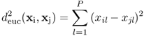
If the sum of the Gaussians, which describe the density of objects in the individual clusters, exactly fits the original data, the entire data set is perfectly described. Each Gaussian can then be considered as one cluster. For the one-dimensional data set presented in Figure 1.1a three Gaussian distributions (dashed lines) are required to obtain a proper fit of the density of objects in the original data (solid line) (24).
Figure 1.1 Example of modeling the density of objects by three Gaussian distributions for (a) one-dimensional and (b) two-dimensional data sets (25).
With the use of multidimensional Gaussian distributions, more complicated data sets can be modeled. The density of objects in a data set consisting of two variables can be modeled by two-dimensional distributions, as illustrated in Figure 1.1b. In this situation also, three clusters are present, and therefore, three distributions are required to obtain a good fit of the object density in the entire data.
The goodness of fit is evaluated by the log-likelihood criterion function, which is given in Equation 1.7 (13). The distributions are weighted by the mixture proportion τk, which corresponds to the fraction of objects in the particular cluster. The log-likelihood depends also on the cluster memberships of each of the N objects. In Equation 1.7, this is expressed as uik, which represents the probability that object xi belongs to cluster k, similar to the membership function given in Equation 1.5. The data set is optimally described by the distributions when the criterion function is maximized (13).
The optimal partitioning of the data is usually obtained by the Expectation-Maximization (EM) algorithm (4, 7, 26). In the first step of EM, the probabilities uik are estimated by an initial guess of some statistical parameters of each cluster. These parameters are the means, covariances, and mixture proportions of the cluster. Subsequently, the statistical parameters are recalculated using these estimated probabilities (4). This process is iterated until convergence of the log-likelihood criterion. The data is eventually clustered according to the calculated probabilities of each object to belong to the particular clusters. It is an advantage that model-based clustering yields cluster memberships instead of assigning each object to one particular cluster. However, because of the random initialization of the parameters, the results of mixture modeling are not robust. Furthermore, the number of distributions to describe the data has to be defined ahead of the clustering procedure (7, 24).
1.2.2.2 Hierarchical Clustering
Another approach to clustering is to obtain a clustering structure instead of a single partitioning of the data. Such a hierarchical clustering can be agglomerative or divisive. The agglomerative strategy starts with assigning each object to an individual cluster (16, 17, 27). Subsequently, the two most similar clusters are iteratively merged, until the data is grouped in one single cluster. Once an object is merged to a cluster, it cannot join another cluster. Divisive hierarchical clustering is similar to the agglomerative strategy, but starts with one cluster that is divided into two clusters that have least similarity. This process is repeated until all clusters contain only one object. Repeated application of hierarchical clustering will result in identical merging or splitting sequences, and thus the results are reproducible (12).
Agglomerative methods are more commonly used. On the basis of the definition of the similarity measure, several variants exist: single, complete, average, and centroid linkage (28, 29). In single linkage, the (updated) distance between the objects of a particular cluster (e.g. c1 and c2) and an object xi is the minimum distance (dmin) between xi and the objects of the cluster. The maximum (dmax) and average (davg) of the distances between the particular object xi and the objects of the cluster is used in complete and average linkage, respectively. In centroid linkage, the distance between an object and the centroid of the cluster (dcen) is used. This is schematically represented in Figure 1.2.
Figure 1.2 Distances between clusters used in hierarchical clustering. (a) Single linkage. (b) Complete linkage. (c) Average linkage. (d) Centroid linkage.

Analogous to the methods based on distance measures, hierarchical clustering can also be performed by model-based clustering. The hierarchical approach is an adaptation from the partitional approach of model-based clustering (12, 23). Model-based agglomerative clustering also starts with individual objects, but merges the pair of objects that lead to the largest increase in the log-likelihood criterion (see Eq. 1.7). This process then continues until all objects are grouped into one cluster (23).
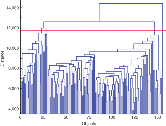
The sequence of merging or splitting can be visualized in a dendrogram, representing, in a treelike manner, the similarity levels at which clusters are merged. The dendrogram can be cut at a particular level to obtain a clustering with a desired number of clusters. The results with different number of clusters can then be easily compared. The dendrogram obtained by average linkage, applied to MR spectra of a patient, is given in Figure 1.3. If, for example, the data should be clustered into four groups, the dendrogram should be cut at a distance of 11,700. This threshold is indicated by the red line in Figure 1.3.
Figure 1.3 Dendrogram showing the sequence of merging MR spectral data by hierarchical clustering. The red line indicates the threshold to obtain four clusters.
Hierarchical clustering methods are not sensitive to outliers because outliers will be assigned to distinct clusters (6). A possible drawback is the computation time. Hierarchical clustering of large data sets will require the merging of many objects: at each merging step, the similarities between pairs of objects need to be recalculated (6, 12, 23, 30).
1.2.2.3 Density-Based Clustering
The third type of clustering methods is based on the density of objects in variable space (7, 19, 31). Clusters are formed by high density areas, and the boundaries of the clusters are given by less dense regions. These densities are determined by a threshold. Another parameter that has to be defined is the size of the volume for which the density is estimated. Objects are then assigned to a cluster when the density within this volume exceeds the predefined threshold. The number of areas with high density indicates the number of clusters in the clustering result. Objects that are not assigned to a cluster are considered as noise or outliers.
DBSCAN is a well-known method to cluster data into regions using high density constraints (19, 22). The algorithm scans an area within a certain radius from a particular object and determines the number of other objects within this neighborhood. The size of the area and the minimum number of objects in the neighborhood have to be defined in advance. If the neighborhood contains more objects than the threshold, then every object in the neighborhood is assigned to one cluster. Subsequently, the neighborhood of another object in the particular cluster is scanned to expand the cluster. When the cluster does not grow anymore, the neighborhood of another object, not belonging to this cluster, is considered. If this object is also located in a dense region, a second cluster is found, and the whole procedure is repeated. With fewer objects in the neighborhood than the threshold, an object is assigned to a group of noisy objects.
Originally, density-based clustering was developed to detect clusters in a data set with exceptional shapes and to exclude noise and outliers. However, the method fails to simultaneously detect clusters with different densities (22). Clusters with a relatively low density will then be considered as noise. Another limitation is the computation time for calculating the density estimation for each object. Moreover, it can be difficult to determine proper settings for the size of the neighborhood and the threshold for the number of objects.
1.2.3 Supervised Pattern Recognition
Pattern recognition can also be supervised, by including class information in the grouping of objects (6, 8). Predefined classes are used by this type of pattern recognition for the classification of unknown objects. For example, the distance of an unidentified object to all the objects in the reference data set can be calculated by a particular distance measure, to determine the most similar (closest) object. The unknown object can then be assigned to the class to which this nearest neighbor belongs. This is the basic principle of the k-nearest neighbor (kNN) method (3, 6, 7). A little more sophisticated approach is to extend the number of neighbors. In that case, there is a problem if the nearest neighbors are from different classes. Usually, a majority rule is applied to assign the object to the class to which the majority of the nearest neighbors belong. If the majority rule cannot be applied because there is a tie, that is, the number of nearest neighbors of several classes is equal, another approach is required. The unknown object can, for example, randomly be assigned to a predefined class. Another method is to assign the object, in this situation, to the class to which its nearest neighbor belongs (7).
Another type of supervised pattern recognition is discriminant analysis (3, 7, 32). These methods are designed to find boundaries between classes. One of the best-known methods is Linear Discriminant Analysis (LDA). With the assumption that the classes have a common covariance matrix, it describes the boundaries by straight lines. More generally, an unknown object is assigned to the class for which the Mahalanobis distance (Eq. 1.3) is minimal. Because the covariance matrices of the classes are assumed to be equal, the pooled covariance matrix is used to calculate the Mahalanobis distances:
1.8 
where Ck and nk are the covariance matrix and the number of objects in cluster k, K is the number of predefined classes, and n is the total number of objects in the data set.
In Quadratic Discriminant Analysis (QDA), the covariance matrices of the classes are not assumed to be equal. Each class is described by its own covariance matrix (3, 7, 32). Similar to LDA, QDA calculates the Mahalanobis distances of unknown objects to the predefined classes and assigns the objects to the closest class. Other more sophisticated techniques also exist, such as support vector machines (33) or neural networks (34), but these approaches are beyond the scope of this chapter.
1.2.3.1 Probability of Class Membership
To reflect the reliability of the classification, the probabilities of class membership could be calculated. This is especially useful to detect overlapping classes. An object will then have a relatively high probability to belong to two or more classes. Furthermore, the probabilities can be used to find new classes, which are not present in the reference data set. If the class membership is low for the predefined classes, the unknown object probably belongs to a totally different class.
The probabilities of class membership can be estimated on the basis of the distribution of the objects in the classes (6, 7). The density of objects at a particular distance from a class centroid is a direct estimator of the probability that an object at this distance belongs to the class. If it is assumed that the data follows a normal distribution, the density of objects can be expressed as in Equation 1.6. If the distance of a new object to a class centroid is known, the density and thus the probability of class membership can be calculated on the basis of Equation 1.6 (3, 7, 32).
A more straightforward approach is based on the actual distribution of the objects, without the assumption that the data can be described by a theoretical distribution (35). In this method, the Mahalanobis distances of the objects in a particular class, say class A, with respect to the centroid of this class are calculated. Also, the Mahalanobis distances of the other objects (not belonging to class A) with respect to the centroid of class A are calculated. This procedure is repeated for every class present in the data set. Eventually, the distances are used to determine the number of objects within certain distances from the centroid of each class. These distributions of objects can be visualized in a plot as presented in Figure 1.4 (36). The solid line represents the percentage of objects from class A within certain Mahalanobis distances (d) from the centroid of class A. Every object of class A is within a distance of 6d from the particular centroid. The dotted line represents the percentage of other objects (not from class A) within certain distances from the centroid of class A. In this example, there is little overlap between objects from class A and the other objects, indicating that class A is well separated from the other classes.
Figure 1.4 Distribution of objects belonging to class A (solid line) and objects belonging to other classes (dotted line) with respect to the centroid of class A (36).
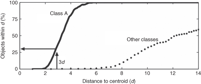
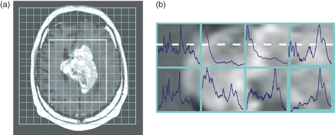
Figure 1.5 Example of the data obtained by MRI and MRS. (a) An MRI image of the brain that clearly shows the presence of abnormal tissue. The grid on the MRI image indicates the resolution of the spectroscopic data. (b) Part of the spectroscopic data, showing the spectra obtained by MRS from several regions of the brain.
The percentage of objects within a particular distance from a class centroid reflects the object density of the class at this distance. Therefore, these percentages can be used to estimate the probabilities of class membership for the classes that are present in the data set. At a distance 3d from the centroid of class A, for example, about 30% of the objects belonging to class A are within this distance. This is illustrated in Figure 1.4. If the Mahalanobis distance of an unknown object with respect to the centroid of class A is 3d, the estimated probability is then 70%. By comparing the probabilities of class membership for each class, the unknown objects can be classified and conclusions can be drawn about the reliability of classification (35).
1.3 Applications
Pattern recognition techniques can be applied to magnetic resonance data to improve the noninvasive diagnosis of brain tumors (37, 38, 39, 40, 41). Because the spectra obtained by MRS are complex, statistical models can facilitate data analysis. The application of pattern recognition techniques to MR spectra and MRI image data is illustrated using research performed on a widely studied data set (24, 35). This data set was constructed during a project called INTERPRET, which was funded by the European Commission to develop new methodologies for automatic tumor type recognition in the human brain (42).
1.3.1 Brain Tumor Diagnosis
Uncontrolled growth of cells is a major issue in medicine, as it results in a malignant or benign tumor. If the tumor spreads to vital organs, such as the brain, tumor growth can even be life threatening (43). Brain tumors are the leading cause of cancer death in children and third leading cause of cancer death in young adults. Only one-third of people diagnosed with a brain tumor survive more than 5 years from the moment of diagnosis (44).
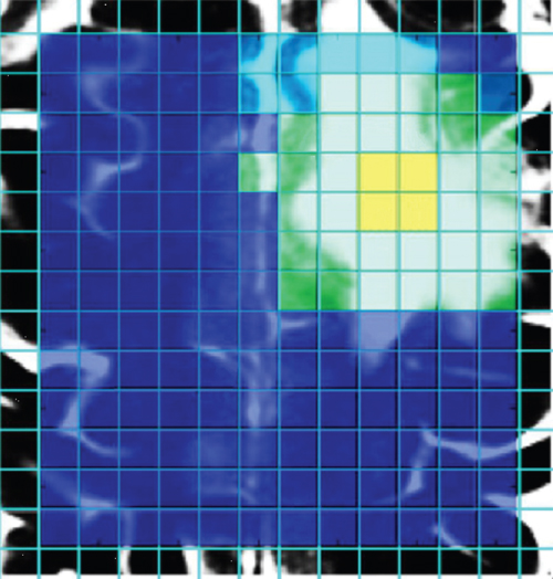
Two commonly used techniques to diagnose brain tumors are magnetic resonance imaging (MRI, Chapter 5) and magnetic resonance spectroscopy (MRS, Section 5.12). MRI provides detailed pictures of organs and soft tissues within the human body (45, 46). This technique merely shows the differences in the water content and composition of various tissues. Because tumorous tissues have a composition (and water content) different from that of normal tissues, MRI can be used to detect tumors, as shown in Figure 1.5a. Even different types of tissue within the same organ, such as white and gray matter in the brain, can easily be distinguished (46).
Magnetic resonance spectroscopy (MRS) is another technique that can be used for diagnosing brain tumors (47, 48, 49). It allows the qualitative and quantitative assessment of the biochemical composition in specific brain regions (50). A disadvantage of the technique is that interpretation of the resulting spectra representing the compounds present in the human tissue is difficult and time consuming. Several spectra acquired from a tumorous region in the brain are presented in Figure 1.5b to illustrate the complexity of the data. To compare the differences in resolution, the MR spectra are visualized on top of the corresponding region of the MRI image. Another limitation of MRS is that the size of the investigated region, for example, of the brain, might be larger than the suspected lesion. The heterogeneity of the tissue under examination will then disturb the spectra, making characterization of the region more difficult (51).
1.3.2 MRS Data Processing
Before chemometrics can be applied to the complex spectra obtained by MRS, these spectra require some processing. Owing to time constraints, the quality of the acquired MR spectra is often very poor. The spectra frequently contain relatively small signals and a large amount of noise: the so-called signal-to-noise ratio is low. Furthermore, several artifacts are introduced by the properties of the MR system. For example, magnetic field inhomogeneities result in distortion of the spectra. Also, patient movement during the MR examinations will introduce artifacts. Another characteristic of the spectra is the appearance of broad background signals from macromolecules and the presence of a large water peak.
1.3.2.1 Removing MRS Artifacts
In order to remove the previously mentioned artifacts, several processing steps need to be performed (26). Different software packages are commercially available to process and analyze MR spectra (43, 52, 53) and, in general, they apply some commonly used correction methods. These methods include eddy current correction (54), residual water filtering (55), phase and frequency shift correction (56), and a baseline correction method (26).
Eddy current correction is performed to correct for magnetic field inhomogeneities, induced in the magnetic system during data acquisition (54, 57). One method to correct for these distortions is to measure the field variation as a function of time. This can be achieved by measuring the phase of the much stronger signal of water. The actual signal can then be divided by this phase factor in order to remove the effect of field variation (57).
Residual water filtering is required to remove the intense water peak that is still present in the spectra after correction for eddy current distortions. A useful filtering method is based on Hankel-Lanczos Singular Value Decomposition (HLSVD) (58). Resonances between 4.1 and 5.1 ppm, as determined by the HLSVD algorithm, are subtracted from the spectra. Water resonates at approximately 4.7 ppm, and therefore, the water peak and its large tails are removed from the spectra without affecting the peak areas of other compounds (55, 58).
Several small phase differences between the peaks in a spectrum may still be present after eddy current correction. In addition, frequency shifts between spectra of different regions, for example, of the brain, may also be present. These peak shifts may be induced by patient movement. A correction method based on PCA can be applied to eliminate the phase and frequency shift variations of a single resonance peak across a series of spectra. PCA methodology is used to model the effects of phase and frequency shifts, and this information can then be used to remove the variations (56, 59).
Broad resonances of large molecules or influences from the large water peak may contribute to baseline distortions, which make the quantification of the resonances of small compounds more difficult. The removal of these broad resonances improves the accuracy of quantification and appearance of the spectrum. Usually, the correction is performed by estimating the baseline using polynomial functions, followed by subtraction from the original signal (26).
1.3.2.2 MRS Data Quantitation
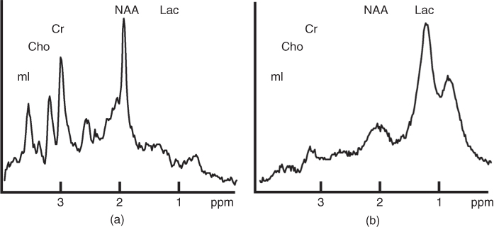
After processing the spectra obtained by MRS, the data can be interpreted. As the spectra contain information from important brain metabolites, deviation in the spectra, and thus in metabolite concentrations, might be indicative of the presence of abnormal tissue. Two different MR spectra are shown in Figure 1.6. The spectrum in Figure 1.6a is acquired from a normal region of the brain and the spectrum in Figure 1.6b originates from a malignant region. The differences between these spectra are obvious and MRS could therefore be used to detect abnormal tissues. Several metabolites are particularly useful for tumor diagnosis, and some of these are creatine (resonates at 3.95 and 3.02 ppm), glutamate (3.75 and 2.20 ppm), glutamine (3.75 and 2.20 ppm), myoinositol (3.56 ppm), choline (3.20 ppm), N-acetyl aspartate (NAA, 2.02 ppm), lactate (1.33 ppm), and fatty acids (1.3 and 0.90 ppm) (25, 60, 61).
Figure 1.6 Two MR spectra, illustrating the difference between spectra obtained from a normal region (a) and a malignant region (b) of the brain. The signals of some metabolites are indicated in the figure: myoinositol (mI) at 3.56 ppm, choline (Cho) at 3.20 ppm, creatine (Cr) at 3.02 ppm, NAA at 2.02 ppm, and lactate (Lac) at 1.33 ppm.
To use the metabolic information in the MR spectra for diagnosis of brain tumors, the intensity of the signals in the spectra requires quantitation (62). A simple approach is to integrate several spectral regions, assuming that each region contains information from one single metabolite. Because some metabolites show overlap in the spectra, for example, glutamate and glutamine, more sophisticated methods could be applied. More accurate methods fit the spectrum by a specific lineshape function, using a reference set of model spectra. A method that has been introduced for the analysis of MR spectra is the LCModel (52, 62, 63). This method analyzes a spectrum as linear combinations of a set of model spectra from individual metabolites in solution. Another powerful tool for processing and quantitation of MR spectra is MRUI (64, 65). This program has a graphical user interface and is able to analyze the MR spectra and present the results in an accessible manner.
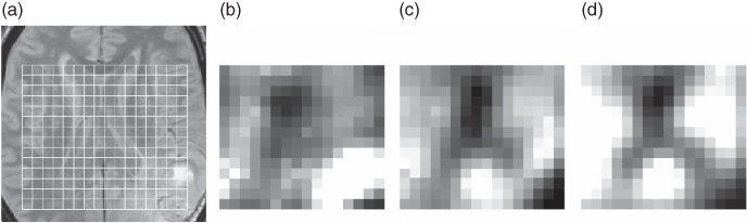
Differences in the quantitated metabolite levels are often used to diagnose the malignancy of a tumor. But even when only the peak intensities of the previously mentioned metabolites are quantitated and interpreted, the amount of data is still large. Especially if MRS is applied to a large region of the brain, to obtain multiple spectra, many metabolite concentrations have to be compared. To facilitate the data analysis, the relative metabolite concentrations within different regions (or actually volumes) could be presented in an image. These regions are referred to as voxels. The resulting metabolic maps visualize the spatial distribution of the concentration of several metabolic compounds, and this can be used to localize or diagnose brain tumors. This is shown in Figure 1.7, in which the relative metabolite concentrations of choline, creatine, and NAA are presented. As shown, an increased concentration of choline is detected in the tumorous region, and reduced concentrations of creatine and NAA are found. Another application of such metabolic maps is to study tumor heterogeneity since this is important for an accurate diagnosis (66, 67, 68).
Figure 1.7 Metabolic maps constructed from MRS data. (a) The MRI image shows the presence of a tumor in the lower right corner of the image. The differences in metabolic concentration are illustrated for (b) choline, (c) creatine, and (d) NAA. Bright pixels represent a high concentration of the particular metabolite.
1.3.3 MRI Data Processing
As mentioned in Section 5.7, the echo time (TE) and the repetition time (TR) are acquisition parameters that determine the T1- and T2-sensitivity of the acquired images. By using different settings for these parameters, different MRI images are obtained (45, 46). Examples of these images are given in Figure 1.8. In the T1- and T2-weighted images (Fig. 1.8a and b), the differences in contrast reveal the ventricles while this is less visible in the PD-weighted image (Fig. 1.8c).
Figure 1.8 MRI images obtained by different acquisition parameters. (a) T1-weighted image. (b) T2-weighted image. (c) Proton density image. (d) T1-weighted image after administration of a gadolinium tracer.
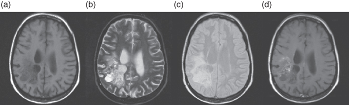
T1-, T2-, and PD-weighted images are commonly acquired with different combinations of TR and TE to be able to discriminate between different tissues. For tumor diagnosis, a contrast medium can be used to improve the tissue differentiation. Usually, gadolinium (Gd) is used as a contrast agent to enhance lesions where the blood–brain barrier is defective. An example of a T1-weighted image enhanced by gadolinium is presented in Figure 1.8d (69).
When the different images need to be compared, they should be aligned with respect to each other. This is necessary because when patients move during the acquisition of the different MRI images, artifacts may be introduced, which complicates the data analysis.
1.3.3.1 Image Registration
Image registration is the alignment of the different images obtained by MRI examinations. This alignment compensates for differences in the position or orientation of the brain in the images due to patient movement. If the images are taken from a series of MRI examinations to study tumor growth or shrinkage after radiation treatment, differences in image size or resolution may be obtained. Image registration should then be applied to match the areas of interest in the images (36).
Although manual alignment of images is possible, it is time consuming and not always reproducible. Automated procedures are therefore preferred. Numerous approaches are available for medical images (69, 70), and in general, they are based on a similarity measure between an image and a corresponding reference image. Because patient movement results in small shifts between different images, a simple cross-correlation method can be used to correct for this artifact (71). However, sensitivity to large intensity differences in different contrast images limits the use of cross-correlation methods. To perform the alignment by matching specific features in the images, which are insensitive to changes in tissue or acquisition, the registration can be improved. These features are, for example, edges and corners in normal brain tissue regions. The chemometric technique Procrustes analysis can then be applied to match the specific features by means of translation, rotation, and uniform scaling transformations. The best match is found when the least-squares solution is obtained by minimizing the distance between all pairs of points in the two images (3, 72).
1.3.4 Combining MRI and MRS Data
If the magnetic resonance data is properly processed, tumorous tissue may be distinguished from normal or other abnormal nonmalignant tissue types, such as necrosis, edema, or scar tissue, by examining the data. However, from the standard acquired MRI images, it is often difficult to properly discriminate tissues within the tumorous region. This can be improved by the contrast-enhanced image, which reveals the lesion where the blood–brain barrier is defective. But because this barrier may variably be affected, the size of the tumor may be under- or overestimated. This has been observed in some brain tumor studies, where the contrast-enhanced lesion was found to be much smaller than the region of abnormal metabolism (73). In addition, MRS examinations have shown that metabolite levels are highly variable for particular tissue types. Also, overlap of metabolite levels between different tumor grades has been observed (73). These findings indicate that MRI and MRS are two complementary techniques for brain tumor diagnosis. MRS provides metabolic information on a low spatial resolution, and MRI provides morphological information on a high spatial resolution. Therefore, the analysis of MRI images and metabolic maps should be performed simultaneously. One of the possibilities is to display a specific metabolic map over an MRI image. Examination of these overlay images facilitates the differentiation between tissue types. For example, the delineation of a viable tumor can be detected more accurately. This is important for studying the effect of chemotherapy or radiation treatment. The combination of MRI and MRS data will improve patient diagnosis and treatment or will facilitate the sampling of biopsies to regions of tumorous tissue.
1.3.4.1 Reference Data Set
For pattern recognition, the data from several patients with a brain tumor and several volunteers was selected from the INTERPRET database (42). After reaching consensus about the histopathology, three tumor types were identified according to the World Health Organization classification system. These three classes contained glial tumors with different grades, indicating the level of malignancy. If a tumor could be assigned to more than one grade, the highest malignancy level determined the grade for the entire tumor, even if most of the tumor is of a lower grade (74). The brain tumors of six patients were diagnosed as grade II, of four patients as grade III, and of five patients as grade IV glial tumors. In addition, classes of normal tissue and Cerebrospinal Fluid (CSF) were created from the patient and volunteer data.
For each predefined class, a selection of voxels from different patients was made. Only voxels from regions that clearly consisted of tissue belonging to the particular class were selected. The data for the normal class was selected from the volunteers or from the contralateral brain region of the patients. The CSF class contained only data from CSF regions that were not in close contact with the tumor region (35).
From the MR spectra of these selected voxels, only the regions where important metabolites appear were selected, as these regions contain most information for the discrimination between brain tumors. The remaining regions contain mainly spectral noise. Besides excluding noise, this also results in a significant reduction in the amount of data.
The estimated metabolite levels should be subsequently combined with the MRI data to improve data analysis (75, 76, 77). However, the spatial resolution of MRI images is much higher than the resolution of MRS data. Therefore, to combine MRI with MRS data, the resolution of the MRI images was lowered to the resolution of the MRS data by averaging the pixel intensities within each spectroscopic voxel. To equally weigh the influence from both data modalities in the classification process, the averaged intensities were scaled to the range of the spectral data.
Different (statistical) methods are available to classify the processed data (see Section 1.2). Application of these methods to the data will result in a classification for each individual voxel. It is also possible to calculate an accuracy measure to indicate the reliability of the classification outcome. An example of a classification method with a statistical basis and the possibility of determining the reliability are discussed in the following sections.
1.3.5 Probability of Class Memberships
After processing the data of the reference set, the distribution of objects in each class can be investigated. By determining the percentage of objects within certain distances from the class centroids, as explained in Section 1.2.3.1, separated and overlapping classes can be found. To investigate which classes are overlapping, the Mahalanobis distance of the objects in each surrounding tissue class with respect to a class centroid was calculated. The surrounding of an isolated class will contain no objects from other classes, whereas the neighborhood of overlapping classes will contain objects belonging to multiple classes. The distributions of the classes in the reference data set are presented in Figure 1.9 (35). Within a distance of about 6d from the centroid of the normal class, every object belonging to this class and some objects from the cerebrospinal fluid class are found. The CSF class shows some overlap with the normal class, but is well separated from the other classes, as depicted in Figure 1.9b. This indicates that the normal and CSF classes are isolated from the tumor classes, and thus, a classification method should discriminate well between normal tissue and malignant tumors.
Figure 1.9 Distribution of the objects in different classes with respect to the centroid of the (a) normal, (b) CSF, (c) grade II, (d) grade III, and (e) grade IV class. The vertical dotted lines indicate thresholds that are used in the classification.
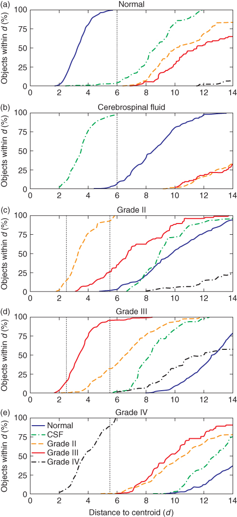
More overlap exists between grade II and III classes. Although at a distance of 5.5d from the centroid of grade II class, almost every object from this class is found; also, about 25% of the objects from grade III class appear within this distance. Less overlap is found with grade IV class. Therefore, discrimination between grade II and grade IV is possible, but grade II class is difficult to be separated from grade III class. The same can be concluded from the distribution of grade III class (Fig. 1.9d). Because grade IV class is isolated from the other classes, this type of tumor can probably be classified with a high reliability (Fig. 1.9e).
1.3.6 Class Membership of Individual Voxels
The distribution of objects can be used to estimate probabilities of class membership for a new patient, as discussed in Section 1.2.3.1. Four patients (A–D) were analyzed; histopathological examination of the brain tissue resulted in the diagnosis of grade III (patient A and D), grade II (patient B), and grade IV (patient C) tumors. The probability maps calculated for the patients are presented in Figure 1.10. Dark voxels in the map represent a high probability that the underlying tissue belongs to the particular class. The probability maps need to be compared regionwise because the probabilities are relative, that is, the intensities are scaled to its maximum value. If a region in the map, for example, of grade II, is dark, while it is bright in the other maps, the estimated probability for grade II class is high (close to 100%). If the region is dark in several maps, the estimated probability of the class membership is lower, and a black pixel does not correspond with a probability of 100%. The probabilities may, therefore, also assist in the assessment of tumor heterogeneity. If the probability is high exclusively for one class, then the tissue will be homogeneous. If the probability is high for two tissue classes, the region might be a mixture of these tissues and might therefore be heterogeneous. However, if a mixture of these two tissues is not possible from a clinical point of view, the high probabilities for both classes indicate a low classification reliability.
Figure 1.10 Probability maps of four patients (A–D). For comparison, an MRI image of each patient is shown on the left. The probability of each voxel to belong to the normal, CSF, grade II, grade III, and grade IV class are shown. Patients A and D are diagnosed with a grade III tumor, patient B with a grade II tumor, and patient C with a grade IV tumor.
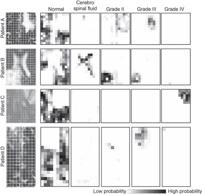
The probability maps for the four patients show that large regions have a high probability to belong to the normal class while these regions have a low probability to belong to another class. The CSF and grade IV regions of the patients show a similar behavior. The voxels with a high probability for the CSF or grade IV class have low probabilities to belong to the other classes. This indicates that these classes are well separated from other classes and that the reliability of classification is high.
Different results are obtained for grade II and grade III classes. The regions where the estimated probability is high for belonging to grade II class also have a high probability to belong to grade III class. In particular, patients A and B show clearly the overlapping problem of these two tissue classes. This could indicate the presence of heterogeneous tumor tissue in these regions and that the reliability of the classification is low.
1.3.7 Classification of Individual Voxels
The estimated probabilities of class membership can be used for classification by assigning each voxel to the class for which it has the highest probability. To define specific classification accuracies, thresholds are set for each class. For a correct classification of 99% of the normal objects, and thus an α-error of 1%, the threshold was set at the position shown in Figure 1.9a. However, with the threshold set at 6d, about 3% of the objects will be classified incorrectly (β-error) as normal. Similar to the normal class, the threshold for the CSF objects was also set at 6d to obtain a low α-error. To minimize the chance that normal or CSF objects are classified as grade IV, the specific threshold for grade IV class was set at 5.5d even though the α-error is then relatively large. Because of the overlap between grade II and III classes, additional thresholds were defined. To obtain a low β-error, an object is directly assigned to grade II when the distance to the particular centroid is very small. With larger distances to grade II class (between 2.5d and 5.5d), the object is assigned to this class only if the distance to grade III class is 1.3 times larger than to grade II class. Otherwise, the object is located in the area of overlap between both classes and the object is assigned to an “undecided” class. The value of 1.3 is obtained after optimization. Identical thresholds are used when the object is closest to grade III class (Fig. 1.9d). If the distance of an object exceeds the specific thresholds for each individual class, the object probably does not belong to any of the classes in the reference data set, and the object is therefore assigned to an “unknown” class.
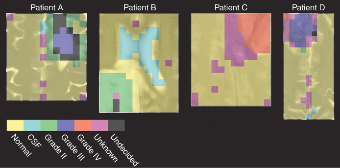
By applying these thresholds to the classification of the four patients A–D, good results are obtained, as shown in Figure 1.11. The results of pattern recognition are projected over different MRI images to compare the results with morphological information. Patient A was diagnosed with a grade III tumor, and the classification result shows the presence of regions of grade II and grade III tumors. But because a tumor is diagnosed by the most malignant tissue present, the result of the statistical method is in agreement with histopathology. From the maps in Figure 1.10, it was clear that some voxels in the tumorous region have equal probability of belonging to grade II and grade III classes. This indicates the presence of a heterogeneous tumor. Therefore, the voxels in the overlapping region of grade II and III tumors are assigned to the undecided class. The voxels in the center of the tumor have the highest probability of belonging to grade III class and are therefore assigned to this class. The tumors of patients B and C are classified as grade II and grade IV tumor in correspondence with the histopathology. Although the tumorous voxels of patient B also have a relatively high probability to belong to grade III class, the estimated probability for grade II class is much higher, and the voxels are classified as grade II. One region of patient C is classified as unknown. This is probably because the particular class is not represented in the reference data set. One voxel of patient D has been misclassified as a grade IV tumor while the patient was diagnosed with a grade III tumor. The reason for this could be that the voxel is a corner voxel, where the MRS signal is low because of the characteristics of the MRS data acquisition.
Figure 1.11 Classification results of patients A–D. Classification was performed by applying specific thresholds to define classification accuracies.
1.3.8 Clustering into Segments
More robust classification results can be obtained by grouping similar voxels in advance of the classification. The voxels that are grouped in one cluster will then be assigned to the same class. The voxels within a region covering a brain tumor, for example, will be grouped in one cluster, and this cluster will subsequently be classified as tumorous tissue. Because a tumor is often larger than the size of a voxel, it could be advantageous to combine the voxels within the tumorous region for classification purposes. However, when the information of the voxels within the tumor is averaged, it is not possible to discover any spatial heterogeneity of the tumor. Therefore, a clustering method that groups only similar voxels instead of grouping neighboring voxels should be applied. One of the methods that could be used to cluster similar voxels is mixture modeling (see Section 1.2.2.1), which describes the spread of the data by a set of distributions. Similar objects will be described by the same distribution and the resulting distributions can be considered as individual clusters. This method is based on a statistical approach, which makes it possible to calculate the probability of an object to belong to a particular cluster. The fit of the data can be evaluated by the likelihood criterion given in Equation 1.7. However, the number of distributions, and thus clusters, has to be defined in advance.
The voxels of a patient are clustered to obtain a partitioning with three, four, five, and six segments. The results for patient A are given in Figure 1.12a (78). The different colors in the clustering results are used only for visualization purpose. Clustering the data into three segments results in one large cluster representing normal tissue and one cluster of tumorous tissue, with a third cluster scattered over the recorded image. If the data is partitioned into more clusters, the voxels covering the tumorous region are divided into multiple segments as illustrated in Figure 1.12a. For example, by clustering the data of patient A into five segments, the tumorous region is covered by three clusters, which could indicate tumor heterogeneity.
Figure 1.12 (a) Results of clustering patient A into three, four, five, and six segments. Clustering was performed by mixture modeling. (b) Estimated probabilities of each segment for each of the five classes. Dark areas correspond to a high probability.
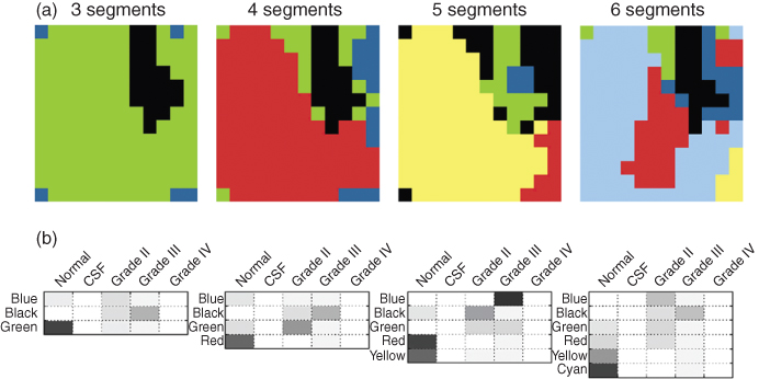
The optimal number of segments can be obtained by comparing the estimated probabilities of class membership. Similar to the calculation for individual voxels, the estimated probabilities can be determined for each segment. This is performed by averaging the MRI and MRS information in each segment. Subsequently, the Mahalanobis distances to the classes in a reference data set are calculated. The estimated probabilities of each segment in the clustering results of patient A are given in the bottom of Figure 1.12b. Each row shows, for a specific segment, the probability of membership for all investigated classes. Dark areas represent high probabilities.
In the three segments solution, the first row represents the probabilities for the blue segment. The probabilities are relatively low, and this could indicate that the blue segment does not belong to any of the classes in the reference data set. The black segment has the highest probability for grade III class, and also some for grade II. The green segment probably contains voxels of the normal class.
In the five cluster solution, more segments are obtained with a high probability for a particular class. Therefore, clustering the patient in five segments is preferred. The blue segment most probably belongs to grade III and the black segment to grade II class. The green segment has a high probability for grade II and III class. The red and yellow segments have a high probability to contain normal tissue.
1.3.9 Classification of Segments
The calculated probabilities can be used to assign each segment to a particular class. With the specific thresholds used in the classification, the result presented in Figure 1.13a is obtained. Each class is color coded according to the legend shown in Figure 1.13. The blue segment of the five cluster solution is classified as grade III and the black segment as grade II (Fig. 1.12). The green segment has equal probabilities to belong to grade II and grade III and is therefore classified as undecided. The red and yellow segments have the highest probability to belong to the normal class, and therefore both segments are classified as normal. Because the probabilities of four segments are high for only one class, the classification of these segments is reliable. The reliability of the green segment is low, or the high probability for more classes could indicate that the underlying tissue is heterogeneous. Overall, the classification indicates that the most malignant tumor of this patient is of grade III, and this is in agreement with the pathology.
Figure 1.13 Results of classification of (a) the segments and (b) the individual voxels. The classification is based on the estimated probabilities for each class.
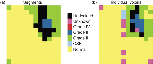
For comparison, the result of the classification of individual voxels is shown in Figure 1.13b. Although the classes after classification of the individual voxels are more scattered and the clustered result seems more robust, both results indicate the presence of a grade III tumor. Because the estimated probability of classification of some segments is higher than any of the probabilities of the individual voxels, it could be advantageous to cluster the data first.
Presented as images, the results of classification could facilitate the diagnosis of brain tumors. The probabilities of class membership are also important as they give an indication about the reliability of classification and/or the heterogeneity of the tissue.
1.3.10 Future Directions
In the procedures described, the data of each voxel was classified without including the spatial relation between voxels. By including the neighborhood information in the classification, the results can be improved (79). In one paper, Canonical Correlation Analysis (CCA) was used to study the effect of including spatial information in the classification of MRS data (80). This technique is based on the correlation between variables (3), for example, MR spectra of a patient and several model (reference) spectra. The problem with heterogeneous tissues is addressed by incorporating mixed spectra of normal and tumorous tissues in the set of model spectra. The application of this approach to the data of patient A results in the classification presented in Figure 1.14, in which distinct regions are obtained. Further details are given in De Vos et al. (80).
Figure 1.14 Classification result of canonical correlation analysis after the inclusion of neighborhood information, applied on the data of patient A. Source: Adapted from Reference (80).
The improvement of the classification accuracy by taking the neighboring voxels into account can be extended further by considering three-dimensional data. This kind of data becomes more widely available with recent developments in the instrumentation. As more neighboring voxels are available in three-dimensional data, more information is used to obtain more robust classification results.
Another future direction could be to combine MRS data with the data obtained from other imaging techniques, such as CT and PET. As other data modalities may contain different information, the fusion of these images may contribute to an improved tumor diagnosis.
1. Beebe KR, Pell RJ, Seasholtz MB. Chemometrics: A Practical Guide. New York: John Wiley and Sons, Inc.; 1998.
2. Massart DL, Vandeginste BGM, Buydens LMC, de Jong S, Lewi PJ, Smeyers-Verbeke J. Handbook of Chemometrics and Qualimetrics: Part A. Amsterdam: Elsevier Science Publishers; 1998.
3. Vandeginste BGM, Massart DL, Buydens LMC, de Jong S, Lewi PJ, Smeyers-Verbeke J. Handbook of Chemometrics and Qualimetrics: Part B. Amsterdam: Elsevier Science Publishers; 1998.
4. Geladi P, Isaksson H, Lindqvis L, Wold S, Esbensen K. Principal component analysis of multivariate images. Chemom Intell Lab Syst 1989;5:209–220.
5. Otto M. Chemometrics, Statistics and Computer Applications in Analytical Chemistry. Weinheim: Wiley-VCH; 1999.
6. Brereton RG. Multivariate Pattern Recognition in Chemometrics, Illustrated by Case Studies. Amsterdam: Elsevier; 1992.
7. Webb A. Statistical Pattern Recognition. Malvern: John Wiley and Sons; 2002.
8. Jain AK, Murty MN, Flynn PJ. Data clustering: a review. ACM Comput Surv 1991;31:264.
9. Fukunaga K. Introduction to Statistical Pattern Recognition. 2nd ed. London: Academic Press; 1990.
10. Richards JA, Jia X. Remote Sensing Digital Image Analysis. Berlin: Springer; 1999.
11. Mao J, Jain AK. A self-organizing network for hyperellipsoidal clustering. IEEE Trans Neural Networks 1996;7:16–29.
12. Fraley C. Algorithms for model-based Gaussian hierarchical clustering. SIAM J Sci Comput 1998;20:270–281.
13. McLachlan G, Peel D. Finite Mixture Models. New York: John Wiley and Sons; 2000.
14. Halkidi M, Batistakis Y, Vazirgiannis M. On clustering validation techniques. J Intell Inf Syst 2001;17:107–145.
15. Noordam JC, van den Broek WHAM. Multivariate image segmentation based on geometrically guided fuzzy C-means clustering. J Chemom 2002;16:1–11.
16. Teppola P, Mujunen SP, Minkkinen P. Adaptive fuzzy C-means clustering in process monitoring. Chemom Intell Lab Syst 1999;45:23–38.
17. Smolinski A, Walczak B, Einax JW. Hierarchical clustering extended with visual complements of environmental data set. Chemom Intell Lab Syst 2002;64:45–54.
18. Liang J, Kachalo S. Computational analysis of microarray gene expression profiles: clustering, classification, and beyond. Chemom Intell Lab Syst 2002;62:199–216.
19. Daszykowski M, Walczak B, Massart DL. Looking for natural patterns in data Part 1. Density-based approach. Chemom Intell Lab Syst 2001;56:83–92.
20. Anderberg MR. Cluster Analysis for Applications. New York: Academic Press; 1973.
21. Bezdek JC. Pattern Recognition with Fuzzy Objective Function Algorithms. New York: Plenum; 1981.
22. Tran TN, Wehrens R, Buydens LMC. Clustering multispectral images: a tutorial. Chemom Intell Lab Syst 2005;77:3–17.
23. Fraley C, Raftery AE. Model-based clustering, discriminant analysis, and density estimation. J Am Stat Assoc 2002;97(458): 611–631.
24. Wehrens R, Simonetti AW, Buydens LMC. Mixture modeling of medical magnetic resonance data. J Chemom 2002;16:274–282.
25. Rijpkema M, Schuuring J, van der Meulen Y, van der Graaf M, Bernsen H, Boerman R, van der Kogel A, Heerschap A. Characterization of oligodendrogliomas using short echo time 1H MR spectroscopic imaging. NMR Biomed 2003;16:12–18.
26. Zandt HJA, van der Graaf M, Heerschap A. Common processing of in vivo MR spectra. NMR Biomed 2001;14:224–232.
27. Pham DL. Spatial models for fuzzy clustering. Comput Vis Image Underst 2001;84:285–297.
28. Li SZ. Markov Random Field Modeling in Image Analysis. Tokyo: Springer-Verlag; 2001.
29. Besag J. On the statistical analysis of dirty pictures. J R Stat Soc Series B-Methodol 1986;48:259.
30. Sneath PHA, Sokal RR. Numerical Taxonomy. London: Freeman; 1973.
31. Yizong C. Mean shift, mode seeking, and clustering. IEEE Trans Pattern Anal Mach Intell 1995;17:790–799.
32. Hastie T, Tibshirani R, Friedman J. The Elements of Statistical Learning, Data Mining, Inference, and Prediction. New York: Springer; 2001.
33. Lukas L, Devos A, Suykens JAK, Vanhamme L, Howe FA, Majos C, Moreno-Torres A, van der Graaf M, Tate AR, Arus C, van Huffel S. Brain tumor classification based on long echo proton MRS signals. Artif Intell Med 2004;31:73–89.
34. Melssen W, Wehrens R, Buydens L. Supervised Kohonen networks for classification problems. Chemom Intell Lab Syst 2006;83:99–113.
35. Simonetti AW, Melssen WJ, van der Graaf M, Postma GJ, Heerschap A, Buydens LMC. A chemometric approach for brain tumor classification using magnetic resonance imaging and spectroscopy. Anal Chem 2003;75:5352–5361.
36. Hutton BF, Braun M, Thurfjell L, Lau DYH. Image registration: an essential tool for nuclear medicine. Eur J Nucl Med 2002;29:559–577.
37. Howells SL, Maxwell RJ, Griffiths JR. Classification of tumour 1H NMR spectra by pattern recognition. NMR Biomed 1992;5:59–64.
38. Preul MC, Caramanos Z, Leblanc R, Villemure JG, Arnold DL. Using pattern analysis of in vivo proton MRSI data to improve the diagnosis and surgical management of patients with brain tumors. NMR Biomed 1998;11:192–200.
39. Tate AR, Majos C, Moreno A, Howe FA, Griffiths JR, Arus C. Automated classification of short echo time in vivo 1H brain tumor spectra: a multicenter study. Magn Reson Med 2003;49:26–36.
40. Szabo de Edelenyi F, Rubin C, Esteve F, Grand S, Decorps M, Lefournier V, Le Bas J, Remy C. A new approach for analyzing proton magnetic resonance spectroscopic images of brain tumors: nosologic images. Nat Med 2000;6:1287–1289.
41. Herminghaus S, Dierks T, Pilatus U, Moller-Hartmann W, Wittsack J, Marquardt G, Labisch C, Lenfermann H, Schlote W, Zanella FE. Determination of histopathological tumor grade in neuroepithelial brain tumors by using spectral pattern analysis of in vivo spectroscopic data. J Neurosurg 2003;98:74–81.
42. INTERPRET. Website by Universitat Autonoma de Barcelona. Last accessed: February 6th, 2012. Available at http://azizu.uab.es/INTERPRET/index.html.
43. Feinberg AP, Ohlsson R, Henikoff S. The epigenetic progenitor origin of human cancer. Nat Rev Genet 2006;7:21–33.
44. National Brain Tumor Society. Website by National Brain Tumor Society. Last accessed: February 6th, 2012. Available at http://www.braintumor.org.
45. Gadian DG. NMR and its Applications to Living Systems. 2nd ed. Oxford: Oxford Science Publications; 1995.
46. Schild HH. MRI Made Easy (… well almost). Berlin: Schering AG; 1990.
47. Andrews C, Simmons A, Williams S. Magnetic resonance imaging and spectroscopy. Phys Educ 1996;31:80–85.
48. Barker PB, Lin DDM. In vivo proton MR spectroscopy of the human brain. Prog Nucl Magn Reson Spectrosc 2006;49:99–128.
49. Gujar SK, Maheshwari S, Bjorkman-Burtscher I, Sundgren PC. Magnetic resonance spectroscopy. J Neuro-Ophthalmol 2005;25(3): 217–226.
50. Stanley JA. In vivo magnetic resonance spectroscopy and its application to neuropsychiatric disorders. Can J Psychiatry 2002;47:315–326.
51. Sibtain NA, Howe FA, Saunders DE. The clinical value of proton magnetic resonance spectroscopy in adult brain tumours. Clin Radiol 2007;62:109–119.
52. Provencher SW. Estimation of metabolite concentrations from localized in vivo proton NMR spectra. Magn Reson Med 1993;30:672–679.
53. van den Boogaart A. MRUI Manual v96.3 A User's Guide to the Magnetic Resonance User Interface Software Package. Delft: Delft Technical University Press; 1997.
54. Klose U. In vivo proton spectroscopy in presence of eddy currents. Magn Reson Med 1990;14:26–30.
55. Vanhamme L, Fierro RD, van Huffel S, de Beer R. Fast removal of residual water in proton spectra. J Magn Reson 1998;132:197–203.
56. Brown TR, Stoyanova R. NMR spectral quantitation by principal-component analysis. II. Determination of frequency and phase shifts. J Magn Reson 1996;112:32–43.
57. Ordidge RJ, Cresshull ID. The correction of transient Bo field shifts following the application of pulsed gradients by phase correction in the time domain. J Magn Reson 1986;69:151–155.
58. Pijnappel WWF, van den Boogaart A, de Beer R, van Ormondt D. SVD-based quantification of magnetic resonance signals. J Magn Reson 1992;97:122–134.
59. Witjes H, Melssen WJ, Zandt HJA, van der Graaf M, Heerschap A, Buydens LMC. Automatic correction for phase shifts, frequency shifts, and lineshape distortions across a series of single resonance lines in large spectral data sets. J Magn Reson 2000;144:35–44.
60. Govindaraju V, Young K, Maudsley AA. Proton NMR chemical shifts and coupling constants for brain metabolites. NMR Biomed 2000;13:129–153.
61. Castillo M, Smith JK, Kwock L. Correlation of myo-inositol levels and grading of cerebral astrocytomas. Am J Neuroradiol 2000;21:1645–1649.
62. Mierisova S, Ala-Korpela M. MR spectroscopy quantitation: a review of frequency domain methods. NMR Biomed 2001;14:247–259.
63. Provencher SW. Automatic quantitation of localized in vivo 1H spectra with LCModel. NMR Biomed 2001;14:260–264.
64. van den Boogaart A. MRUI Manual v.96.3. A User's Guide to the Magnetic Resonance User Interface Software Package. Delft: Delft Technical University Press; 2000.
65. Naressi A, Couturier C, Castang I, de Beer R, Graveron-Demilly D. Java-based graphical user-interface for MRUI, a software package for quantitation of in vivo/medical magnetic resonance spectroscopy signals. Comput Biol Med 2001;31:269–286.
66. Fulhan MJ, Bizzi A, Dietz MJ, Shih HHL, Raman R, Sobering GS, Frank JA, Dwyer AJ, Alger JR, Di Chiro G. Mapping of brain tumor metabolites with proton MR spectroscopic imaging: clinical relevance. Radiology 1992;185:675–686.
67. Furuya S, Naruse S, Ide M, Morishita H, Kizu O, Ueda S, Maeda T. Evaluation of metabolic heterogeneity in brain tumors using 1H-chemical shift imaging method. NMR Biomed 1997;10:25–30.
68. Segebarth C, Balériaux D, Luyten PR, den Hollander JA. Detection of metabolic heterogeneity of human intracranial tumors in vivo by 1H NMR spectroscopic imaging. Magn Reson Med 1990;13:62–76.
69. Weinmann HJ, Ebert W, Misselwitz B, Schmitt-Willich H. Tissue-specific MR contrast agents. Eur J Radiol 2003;46:33–44.
70. Maintz JBA, Viergever MA. A survey of medical image registration. Med Image Anal 1998;2:1–36.
71. Pratt WK. Digital Image Processing. New York: John Wiley & Sons; 1978. pp. 526–566.
72. Evans EC, Collins DL, Neelin P, MacDonald D, Kamber M, Marret TS. Three-dimensional correlative imaging: applications in human brain imaging. In: Thatcher RW, Hallett M, Zeffiro T, John ER, Huerta M, editors. Functional Neuroimaging: Technical Foundations. Orlando: Academic Press; 1994. pp. 145–161.
73. Nelson SJ, Vigneron DB, Dillon WP. Serial evaluation of patients with brain tumors using volume MRI and 3D 1H MRSI. NMR Biomed 1999;12:123–138.
74. American Joint Committee on Cancer. AJCC Cancer Staging Manual. 6th ed. New York: Springer; 2002.
75. Simonetti AW, Melssen WJ, Szabo de Edelenyi F, van Asten JA, Heerschap A, Buydens LMC. Combination of feature-reduced MR spectroscopic and MR imaging data for improved brain tumor classification. NMR Biomed 2005;18:34–43.
76. Devos A, Simonetti AW, van der Graaf M, Lukas L, Suykens JAK, Vanhamme L, Buydens LMC, Heerschap A, van Huffel S. The use of multivariate MR imaging intensities versus metabolic data from MR spectroscopic imaging for brain tumour classification. J Magn Reson 2005;173:218–228.
77. Galanaud D, Nicoli F, Chinot O, Confort-Gouny S, Figarella-Branger D, Roche P, Fuentes S, Le Fur Y, Ranjeva JP, Cozzone PJ. Noninvasive diagnostic assessment of brain tumors using combined in vivo MR imaging and spectroscopy. Magn Reson Med 2006;55:1236–1245.
78. Simonetti AW. Investigation of brain tumor classification and its reliability using chemometrics on MR spectroscopy and MR imaging data. [PhD thesis]. Radboud University Nijmegen, Nijmegen; 2004. pp. 115–137.
79. Krooshof PWT, Tran TN, Postma GJ, Melssen WJ, Buydens LMC. Effects of including spatial information in clustering multivariate image data. Trends Anal Chem 2006;25(11): 1067–1080.
80. de Vos M, Laudadio T, Simonetti AW, Heerschap A, van Huffel S. Fast nosologic imaging of the brain. J Magn Reson 2007;184:292–301.