
Chapter 11
Biomedical Sonography
11.1 Basic Principles
11.1.1 Introduction
Ultrasound imaging was first introduced in 1950 by (Wild 1950) together with Reid. Since then, it developed to one of the most important diagnostic imaging modalities. With today's scanners, two-dimensional cross-sectional images of the body can be produced in real time with a spatial resolution below 1 mm. Ultrasound imaging relies on the propagation of mechanical waves with frequencies beyond the audible range into the body, the reflection and scattering of sound by tissue structures, and the registration of the echoes. Similar to sonar and radar, it is a pulse-echo ranging technique. Using the acoustical Doppler effect, the quantitative measurement of blood flow is possible, and flow velocity and direction can be presented in real time as colored overlays. To enhance the echoes from blood, ultrasound contrast media were developed. They show nonlinear behavior that can be used for their specific and sensitive detection. With the introduction of nonlinear imaging modes for contrast media also, nonlinear imaging of tissue became of interest and showed a significant improvement in many imaging situations. Recently, the higher integration of electronics and the increasing computer power led to the realization of real-time three-dimensional imaging, which is of special interest in cardiological applications.
After more than 50 years of development, ultrasound imaging is still enabling new applications, for example, by imaging of molecular markers with targeted contrast media or by the combination of imaging and therapy with local drug delivery.
11.1.2 Ultrasonic Wave Propagation in Biological Tissues
Ultrasound is a mechanical wave characterized by small pressure variations ![]() and a material displacement
and a material displacement ![]() propagating at the speed of sound c at frequencies beyond the hearing range. In biomedical sonography, typically frequencies in the range from 1 to 20 MHz are used for human examinations. In special applications such as imaging in dermatology, ophthalmology, or for small-animal imaging, higher frequencies up to 100 MHz are also common.
propagating at the speed of sound c at frequencies beyond the hearing range. In biomedical sonography, typically frequencies in the range from 1 to 20 MHz are used for human examinations. In special applications such as imaging in dermatology, ophthalmology, or for small-animal imaging, higher frequencies up to 100 MHz are also common.
Soft tissues can be modeled as liquids in the respect that only longitudinal waves with the direction of displacement equal to the direction of propagation exist. The material can be described by its density ρ and compressibility κ. The propagating wave is characterized by its pressure ![]() and the particle velocity
and the particle velocity
11.1 ![]()
Often it is more convenient to use the velocity potential ϕ:
11.2 ![]()
For small pressure variations, the wave equation can be linearized and holds in similar form for the pressure, the components of the displacement velocity, as well as for the velocity potential:
where the speed of sound
11.4 ![]()
The most important solutions to this equation are forward and backward traveling plane waves
11.5 ![]()
In this, the wave vector ![]() determines the direction of propagation
determines the direction of propagation
11.6 ![]()
where λ is the wavelength, the angular frequency ω = 2πf, and f is the frequency of the ultrasound wavef. Wavelengths in water are in the range from 0.1 to 1 mm for the clinically used frequency range of 1.5 to 15 MHz. Pressure and particle velocity of the forward traveling plane wave have a fixed ratio, the acoustic impedance of the material
11.7 ![]()
The acoustic impedance determines the reflection coefficient at a boundary between two media. For a wave traveling from a material with Z1 to a material with Z2 the amplitude reflection factor is
11.8 ![]()
where p1B and p1F are the pressure amplitudes of the backward and forward traveling wave in material 1, respectively.
Ultrasonic imaging is based on the fact that soft tissues show only small variations in their acoustic impedance. Therefore, only a small amount of energy is reflected, which allows most of the wave's energy to propagate further into tissue. Table 11.1 shows average values of speed of sound and acoustic impedance for some tissues. A comprehensive overview of acoustical tissue parameters is given by Duck (1990). The soft tissue average is considered to be 1540 m s−1 and is used by most ultrasound scanners to calculate echo range from the time of echo arrival. Note that the large compressibility of air leads to an acoustic impedance close to zero. Thus, tissue–air boundaries will reflect sound totally.
Table 11.1 Speed of Sound and Acoustic Impedance for Tissues (Duck, 1990)
| Speed of Sound | Acoustical Impedance in | |
| Material | (m s−1) | MRayls = 106 kg m−2 s−1 |
| Air | 330 | 0.0004 |
| Water (20°C) | 1480 | 1.48 |
| Fat | 1450 | 1.38 |
| Liver | 1570 | 1.65 |
| Muscle | 1580 | 1.70 |
| Bone | 3500 | 7.80 |
| Soft tissue average | 1540 | 1.63 |
11.1.3 Diffraction and Radiation of Sound
The sound field emitted from a vibrating surface can be derived by Huygen's principle: each point on the transducer aperture emits a spherical wave into the medium, and the resulting pressure field is the superposition of the infinitesimal contributions of all source points. The mathematical formulation of this principle is the Rayleigh-Sommerfeld integral. For a sound-emitting aperture in a rigid baffle, it integrates over all source points on the transducer surface S to calculate the complex amplitude of the pressure for harmonic excitation at frequency ω (Morse and Ingard, 1968):
Here, ![]() is the distribution of the complex amplitude of the velocity component normal to the emitting surface. The time varying pressure is related to the complex amplitude by
is the distribution of the complex amplitude of the velocity component normal to the emitting surface. The time varying pressure is related to the complex amplitude by
11.10 ![]()
This superposition results in field patterns that often can be calculated only by numerically solving Eq. (11.9). For example, the simulation software Field II developed by Jensen (1991) for MATLAB was used to produce the sound field simulations in the figures of this chapter.
In many situations, it is useful to analyze far field properties for which the Fraunhofer approximation holds. The far field distance is
11.11 ![]()
where A is the transducer area and λ is the wavelength. When the transducer is placed in the origin of a spherical coordinate system, the field distribution on a sphere with radius much greater than dfar will be the Fourier-transform of the aperture velocity distribution:
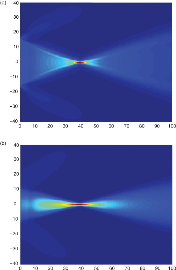
The apertures used for ultrasonic imaging are usually rectangular elements within an array of transducers. Thus, in the far field, the pressure distribution is a sinc function when all active array elements are pulsed with the same voltage, that is, energy is transmitted also in the side lobes. The side lobes in the diffraction pattern can be seen in Figure 11.1. Here, the maximum pressure of the sound field in front of a rectangular aperture built by 128 array elements with half-wavelength spacing and a total width of 28.1 mm is shown. In Figure 11.1a, the array elements are excited with identical pulses with a center frequency of 3.5 MHz. The pulses are time delayed to arrive at the focus at 40 mm at the same time. Clearly, side lobes can be seen behind the focus of the sound beam. In contrast, Figure 11.1b shows no side lobes. Here, the pulse amplitudes of the 128 elements are weighted with a Hanning function (apodization). However, the focusing is weaker because of apodization.
Figure 11.1 Sound field of a group of 128 rectangular array elements with half-wavelength spacing pulsed with a center frequency of 3.5 MHz. In (a), all elements are pulsed with the same amplitudes and are delayed for a focus in 40 mm distance. In (b), the focusing is identical, but the element amplitudes are varied with a Hanning window function over the length of the array. This leads not only to fewer side lobes but also to increased main lobe width and thus reduced spatial resolution in the lateral direction. Scales are in millimeters.
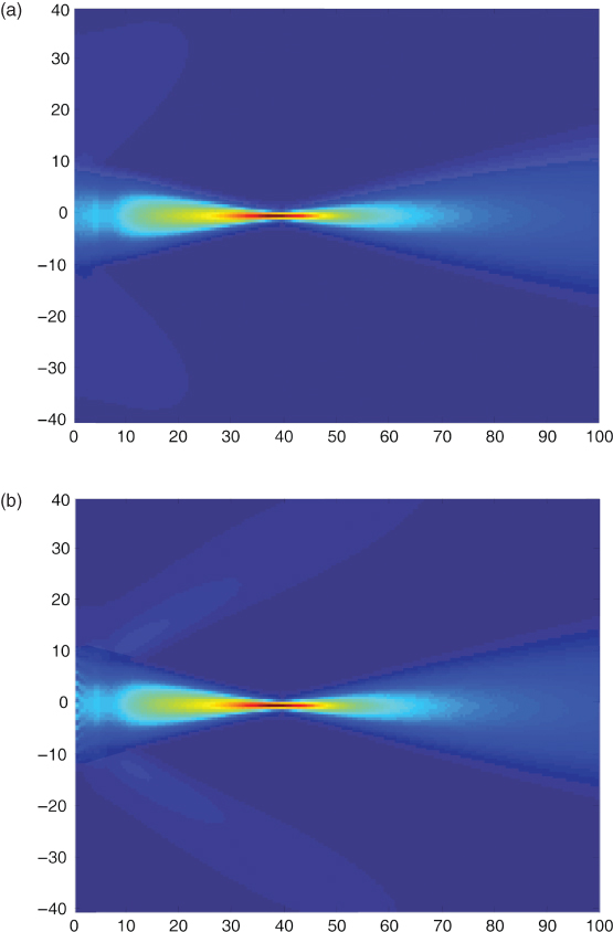
In Figure 11.2, the effect of element spacing of a transducer array is demonstrated. While an element spacing of one wavelength as in Figure 11.2a is still acceptable for linear array imaging, arrays with larger element spacing such as 1.5 wavelengths in Figure 11.2b show strong grating lobes, which can be explained by Eq. (11.12) in the far field as the Fourier transform of the periodic element structure. In imaging, grating lobes and side lobes will decrease imaging contrast because the system is sensitive to scatterers that lie off the main focusing direction. Usually, imaging arrays of high end systems have less than one wavelength spacing. The examples show that the design of transducer arrays and the pulsing schemes are crucial for the focusing of the sound beam and thus for image resolution.
Figure 11.2 Effect of the variation of element spacing in a transducer array. Total transducer size and pulsing is kept identical to Figure 11.1(b), but element spacing is (a) one wavelength with 64 elements and (b) 1.5 wavelengths with 43 elements. Clearly, increasing grating lobes are visible.
11.1.4 Acoustic Scattering
Early ultrasonic imaging devices had a limited dynamic range and could only show reflections from tissue boundaries. However, also small fluctuations of density and compressibility at spatial dimensions at the scale of the wavelength or below scatter the sound waves. Modern ultrasound scanners have enough dynamic range to measure and display these backscattered signals. In fact, scattering from tissue provides most of the image information. Objects much larger than the wavelength show specular reflection. If the length scale of density and compressibility changes is in the range of the wavelength, resonances and complicated backscatter behavior arise. This can be seen for the example of a spherical solid elastic scatterer in water, one of the few geometrical objects for which an analytical expression of the scattered field was derived (Hickling, 1962). When scattering structures become much smaller than the wavelength of the incident wave, Rayleigh scattering is observed. Biological tissues are multiscale structures that show all of the different scattering domains simultaneously. So far, a general model for the acoustic description of biological tissue is not available. An appropriate model for the Rayleigh scattering in biological tissues can be given by modeling tissue as random fluctuations of the relative acoustic impedance (Schmitz, 2002)
11.13 ![]()
described by its zero mean value and its autocovariance function
11.14 ![]()
where E denotes statistical expectation. The backscattering strength of the random medium is described by its backscattering coefficient (Schmitz, 2002), which can be calculated from the autocovariance function by Fourier-transformation:
11.15 
Its unit is per meter, and when integrated over a scattering volume, it gives the differential scattering cross section, which gives the ratio of scattered power per steradian to the incident intensity and has units of square meters. It can also be seen that the case of an ideal point scatterer can be considered by
11.16 ![]()
and results in a constant integral and in the backscatter coefficient increasing with k4, as known for Rayleigh scattering.
Although scattering is the cause of most of the signal power received by ultrasound scanners, it is difficult to quantify it absolutely for the purpose of tissue characterization. This is because of the unknown attenuation of intervening tissue and the dependency on the imaging system's transfer function. There have been many research efforts to analyze backscatter and its frequency dependence quantitatively to detect, for example, malignant tumors of the breast, the prostate, or the parotid gland.
11.1.5 Acoustic Losses
The wave equation, Eq. (11.3), does not include losses. In biological tissues, the relative attenuation per wavelength is small. Therefore, the attenuation can be accounted for by an additional exponential decay term for the wave amplitude. In the case of a wave propagating in the z-direction, the amplitude depends on the distance z according to
11.17 ![]()
Here, α(f) is the frequency-dependent attenuation in Nepers per centimeter. Often, attenuation is given in dB cm−1 as defined by a(f). The frequency dependence of biological tissues can be described most correctly by a power law
11.18 ![]()
with exponents y close to one, different from the attenuation in water with y = 2. Ultrasound scanners typically use a limited frequency range, in which the attenuation can be approximated well to be linear with frequency
11.19 ![]()
The linear attenuation coefficient is in the order of 0.5 dB MHz−1cm−1 for soft tissues. For a typical frequency of 4 MHz and a penetration depth of 5 cm, to which sound has to travel and return, a total attenuation of 0.5 dB MHz−1cm−1 · 4 MHz · 2 · 5 cm = 20 dB, that is, a tenth in amplitude, is expected. Considering the small reflection and backscatter coefficients in tissue, ultrasound receivers have to be very sensitive, because the maximum transmit amplitudes are limited by the onset of possible bioeffects. The total attenuation is caused by absorption and scattering, the latter accounting only for less than 15% (Bamber, 1998; Shung and Thieme, 1993).
11.1.6 Doppler Effect
When sound is transmitted and reflected or scattered by an object moving with speed v, the received sound wave is shifted in frequency. If the transmitter and receiver are in the same position and the speed of the scattering object is small compared to the speed of sound c, the frequency shift is
where θ is the angle θ between the direction of sound propagation and the direction of the object movement. This effect can be used to measure blood flow by detecting the frequency shifts of ultrasound waves scattered back by red blood cells or ultrasound contrast media. For quantitative measurements, the angle between blood flow and sound propagation has to be measured interactively by the user. For physiological blood flow velocities (up to 3 ms−1 in the ascending aorta) the Doppler shifts are in the audible frequency range and can be listened to on most ultrasound imaging systems with Doppler capability.
Since blood flow velocity varies over the cross section of a blood vessel, a distribution of different velocities will be observed as a distribution of Doppler frequency shifts. Thus, a spectral decomposition of the Doppler signal allows measuring the velocity distribution within a vessel. Different Doppler measurement techniques are realized in diagnostic scanners and are discussed in more detail later.
11.1.7 Nonlinear Wave Propagation
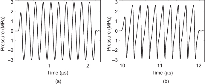
The linear wave equation holds only for small sound pressures when it can be assumed that the material's density is proportional to the pressure. Modern diagnostic ultrasound scanners can reach local peak values of the intensity exceeding 100 W cm−2, and the assumption of linearity is no longer valid. In this case, the transmitted waveform is deformed by a nonlinear transformation, leading to the generation of harmonic frequencies. In Figure 11.3, the effect on a sine-burst pulse with a center frequency of 1 MHz transmitted through 40 cm of water and measured by a hydrophone is demonstrated. The generation of higher harmonic frequencies by nonlinear propagation in tissue is used in Tissue Harmonic Imaging (THI) and often gives clearer images with higher resolution and better delineation of tissue boundaries.
Figure 11.3 Simulation of the nonlinear wave propagation in water from an unfocused piston transducer excited with a 10-cycle sine burst. The waveform in (a) is observed at a distance of 0.3 mm to the transducer and shows a maximum peak pressure of 3 MPa. The waveform in (b) is measured at a distance of 15 mm and clearly shows the deviation from the sinusoidal waveform due to nonlinear propagation.
11.1.8 Biological Effects of Ultrasound
11.1.8.1 Thermal Effects
The absorption of ultrasound in tissue leads to a temperature increase that depends on the average intensity of the sound field. To give an indication of the temperature rise that can be expected in tissue, diagnostic ultrasonic scanners have to present a Thermal Index (TI) on the screen as part of the Output Display Standard (ODS). The TI is the ratio of the actual system power to the power needed to raise the temperature in the hottest spot of a model medium by 1°. If the TI is smaller than 0.4, it does not have to be displayed. Different TI calculations exist for soft tissue (TIS), bone (TIB), and cranial applications (TIC) in scanned and nonscanned modes. They all assume specific models that represent worst case scenarios and might not be the same as the actual scanning situation. Thus, the TI gives no measurement of the actual temperature increase but an indication of a possible risk of such an increase.
11.1.8.2 Cavitation Effects
A second effect that can be hazardous to tissue is the creation of cavitation. Cavitation may occur in the rarefactional phase of the pressure wave. It is more likely to occur if cavitation nuclei, for example, gas microbubbles, are present in the tissue. It has been shown that tissue tolerates negative pressures better at higher frequencies, and the Mechanical Index (MI) was introduced to give an indication of cavitation risk:
11.21 ![]()
where p−max is the maximum rarefactional pressure in megapascals and fc is the center frequency in megahertz. The MI is dimensionless and takes the value of one for a maximum rarefactional pressure of 1 MPa at a frequency of 1 MHz. The MI is limited at 1.9 by the Us Food and Drug Administration (FDA), and values smaller than 0.4 do not have to be displayed. For ultrasound contrast media that consist of gas microbubbles, cavitation and additional effects such as cell membrane opening can occur and are still under investigation.
11.2 Instrumentation of Real-Time Ultrasound Imaging
11.2.1 Pulse-Echo Imaging Principle
Ultrasound imaging is based on the pulse-echo principle: a short sound pulse is transmitted into tissue from a focused transducer. The pulse propagates in the tissue with the speed of sound and is reflected and scattered at inhomogeneities of the acoustic material parameters. The echoes travel back to the transducer that has been switched to receive mode after transmitting the pulse. The focusing of the transducer restricts the energy of the propagating sound wave to approximately a line in a certain range around the focal depth. Current piezoelectric transducers emit short sine wave bursts with approximately a Gaussian envelope. The depth of the echo origin z can be calculated from the travel time t by
11.22 ![]()
using the average speed of sound in tissue of 1540 m s−1. A single scan line of echoes from a tissue is shown in Figure 11.4. Early medical ultrasound equipment showed such scan lines on an oscilloscope for inspection by the clinician, for example, to detect a midline shift in the brain. This representation of echo data is called an A-line or A-scan because the amplitude of the signal is shown. Owing to attenuation, the amplitude of the signal decays over increasing depth. Ultrasound scanners counteract with increasing the gain of the receive amplifiers with time. This Time-Gain Compensation (TGC) or Depth-Gain Compensation (DGC) is performed before analog signals are sampled and digitized to increase the dynamic range of the scanning equipment. However, in modern high end scanners, the TGC available as a setting to the clinical user is only an additional postprocessing method working on digitized data.
Figure 11.4 A-scan line of echoes from tissue and envelope signal without high frequency carrier signal.
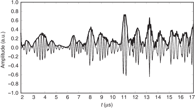
The information about echo strength is only contained in the envelope of the A-scan data, which can be calculated by envelope detection. The envelope of one A-scan line represents the echo strengths of objects along one line in the tissue. By moving the transducer, this line can be scanned, and a cross-sectional image of tissue is formed, in which the brightness represents the echo strength of image points. Therefore, this cross-sectional image is called a B-scan for brightness scan. The movement of the scan line can be realized by a mechanical translation or rotation of a single element transducer, as it was common in the first B-scan equipment. In today's clinical scanners, the transducer movement is realized by electronic switching of active elements of an array of small transducers as well as electronic beam forming and beam steering discussed in Section “Beamforming”.
11.2.2 Ultrasonic Transducers
Currently, diagnostic ultrasound scanners use only piezoelectric transducers to generate sound waves. The scanhead of a diagnostic ultrasound scanner contains up to a few hundred transducer elements in linear arrays and up to thousands of elements in 2D arrays. The elements are driven with pulses with different time delays to influence the characteristics and directions of the sound beams interrogating the object of interest.
One transducer element consists of a piezoelectric ceramic, a typical material being lead zirconium titanate (PZT). The transducer is connected by metal electrodes on both sides as shown in Figure 11.5. The thickness of the transducer element is half the wavelength of sound in the ceramic material for the center frequency. This makes the transducer resonant at the center frequency. The better the quality of the resonance, the more sensitive the transducer is. However, in this case, it transmits only long ringing pulses, rendering pulse-echo measurements with high resolution impossible.
Figure 11.5 Part of a linear transducer array showing six piezoelectric transducer elements. The distance between element centers is the array pitch, and the element separation is the kerf. Sound is transmitted through quarter wavelength matching layers and an acoustical lens that focuses in the elevation direction perpendicular to the imaging plane. The backing attenuates sound transmitted to the back of the transducer.
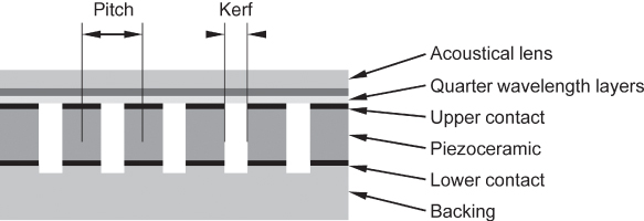
Acoustic losses are introduced by the sound wave radiated into the medium at the front and even more by the backing material (Fig. 11.5). Owing to this, the resonance is less pronounced. This gives the transducer a larger bandwidth and enables it to emit short pulses. Thus, transducer design is a compromise between the sensitivity of the transducer and its bandwidth. Actual transducers reach bandwidths of up to 100% of the center frequency. Often, the band limits of a transducer array can be deduced from its name, but no standard naming convention is used: for instance, a Philips L8-4 transducer is a linear array transducer with a bandwidth from 4 to 8 MHz.
The quality of an imaging array is also characterized by the size and spacing of the elements. The element pitch is the distance between element centers, and the kerf is the space between elements. As discussed earlier, element pitch should typically be less than the wavelength in water at the center frequency.
A severe problem of piezoelectric transducers is the strong mismatch of acoustic impedances between the transducer material (ca. ZP = 34 MRayls) and tissue (ca. ZW = 1.5 MRayls). Owing to this, most of the acoustic energy would be reflected at the transducer surface. Therefore, quarter wavelength matching layers are used. If one-quarter wavelength layer is used, its acoustic impedance is chosen as ![]() , and no reflections are observed at the frequency for which the layer has quarter wavelength. For broadband pulses as used in ultrasound imaging, the matching is not perfect for frequencies away from the matching frequency, and the matching layer will limit the bandwidth of the transducer.
, and no reflections are observed at the frequency for which the layer has quarter wavelength. For broadband pulses as used in ultrasound imaging, the matching is not perfect for frequencies away from the matching frequency, and the matching layer will limit the bandwidth of the transducer.
With higher electronic integration and increasing computer power, fully connected two-dimensional arrays also become available. This trend in increasing element counts and the need for the integration of electronics with the elements boosts development of novel transducer technology that is based on Microelectromechanical Systems (MEMS).
The most prominent new transducer design is the Capacitive Micromachined Ultrasound Transducer (CMUT), in which a thin metalized membrane covers a small gap to a second electrode as shown in Figure 11.6. If a voltage is supplied to the electrodes they will be attracted to each other by electrostatic forces, irrespective of the poling of the voltage. This nonlinear behavior is overcome by a bias DC voltage that brings the membrane into a working point and a small high frequency excitation around this point. If the DC voltage rises over a certain threshold where attractive electrostatic forces grow faster than the elastic forces pulling the membrane back, the membrane will collapse and touch the bottom of the transducer. Then, it can be released only when the voltage is lowered far beyond the collapse voltage. Theoretically, such transducers can reach very high coupling factors when driven close to the collapse point. However, parasitic capacitances limit the coupling factor in practice.
Figure 11.6 Micromachined transducers: principle of (a) capacitive micromachined ultrasound transducers (CMUT) and (b) piezoelectric micromachined ultrasound transducers (PMUT).
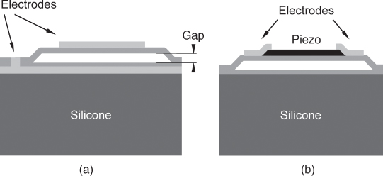
A different principle under investigation is the Piezoelectric Micromachined Ultrasound Transducer (PMUT), in which a piezoelectric thin film layer bends an elastic membrane (Fig. 11.6b). This principle has the advantage that it does not need a DC bias voltage and is more compatible with current scanner electronics.
Both technologies have the advantage that they use membranes with very low mechanical impedances that do not need any match to the tissue. Therefore, these transducers have a much larger bandwidth than conventional piezoelectric transducers. However, sensitivity and reliability are still an issue for both MUT principles. At the moment, manufacturers of diagnostic ultrasound equipment are still evaluating these technologies for the use in commercial equipment.
11.2.3 Beamforming
11.2.3.1 Beamforming Electronics
To focus sound beams and to direct them along different lines into tissue, the spatial distribution of the amplitude and phase of the emitting transducer excitation has to be controlled with respect to amplitude and phase. This is realized by the use of array transducers that consist of numerous small transducer elements. Several neighboring transducer elements of the array transducers build the active aperture. The transducer elements of such a group are driven all individually with different phases (delays) and amplitudes. In receive mode, the signals are also measured for each single element of the active aperture.
For this reason, current ultrasound scanners have about 64–256 parallel transmit and receive channels in the case of two-dimensional imaging with one-dimensional arrays. For three-dimensional imaging with two-dimensional arrays, even more channels are necessary, but because of cost, compromises are often made in 3D imaging. Transmitters are typically able to excite only rectangular pulses of positive and negative transmit voltages that will be bandlimited by the transducer transfer function. In high end systems, the transmit voltages can be adjusted for individual elements. The delay of the pulses to the elements is controlled digitally. In the receive mode, the echoes are amplified using TGC to account for tissue attenuation and digitized. The receive beamforming is then realized by digital signal processing of the individual echoes.
11.2.3.2 Array Beamforming
In array beamforming, the transducer elements are pulsed with individual delays, in such a way that the waves from the single elements reach the focal point F simultaneously (Fig. 11.7). Around this focal point, the sound wave propagation is nearly restricted to a line. The transmit focal point is fixed for one transmit/receive cycle. Often, more than one transmit focus is used in several transmit/receive cycles to combine the resulting images focused to different depths.
Figure 11.7 Linear array beamforming in transmit mode: a subgroup of the transducer array is active and focused to a fixed depth by the pulse delays realized in the beamformer. At the focus, waves of all elements arrive at the same time. The scan-line position can be moved by electronically switching to another subgroup of elements. The focus can be adapted by the choice of beamformer delays. In the background, a simulation of the maximum sound pressure is shown.
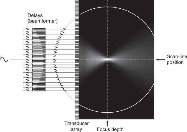
In the receive case, the echoes from a field point P will reach the transducer element with known differences in arrival times. The receiver is focused on point P by delaying the echoes in such a way that they are aligned in time and then summing the signals. In receive beamforming, the delays, and thus point P, can be adapted dynamically to the origin of echoes. Knowing the average speed of sound in tissue, the origin of echoes can be calculated by the time the transmit pulse needs to reach P and return to the transducer. Together with dynamic receive focusing, some scanners also enlarge the active aperture (dynamic aperture) for increasing depth to keep the focal point size constant.
With one-dimensional arrays, focusing perpendicular to the imaging plane (often named elevational focusing) cannot be realized electronically. Therefore, an acoustic lens with a fixed focus is used. With two-dimensional arrays, the elevational focus can also be realized by electronic beamforming, even if only a few elements (e.g., 5) in the second dimension are used. Such arrays are called 1.5D arrays, in contrast to full two-dimensional arrays with equal element numbers and sizes in both dimensions as used for 3D imaging.
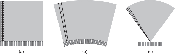
After recording one scan line, the position of the scan line has to be changed to gather image information along more lines. Two different principles exist to change the scan-line position: linear array scanning and phased array scanning. In linear array scanning, a subgroup of elements of a long array is active, and after recording one scan line, the active group is moved electronically along the array. By this, parallel scan lines are acquired (Fig. 11.8a). In some array designs, the elements are arranged on an arc to give a convex scan (Fig. 11.8b). However, the scan principle is the same. In phased array scanning, the focal points in transmit and receive are not on a line perpendicular to the transducer surface, but they are on a line steered under a steering angle ϕ. After one scan line is recorded, the steering angle is changed. Thus, a sector geometry with scan lines originating from one point on the transducer is generated (Fig. 11.8c). Which scan geometry is preferred depends on the application and the access to the organ of interest.
Figure 11.8 Different scan geometries in current diagnostic ultrasound scanners: (a) linear scan, (b) convex scan, and (c) phased array sector scan.
The phased array scan can also be used to sample volumes when a two-dimensional array is used to create a pyramid volume of scan lines originating in the transducer center. However, even for only 64 elements in one direction, a fully connected array would need 4096 individual channels. Therefore, first real-time 3D scanners used sparse random arrays in which only a random pattern of elements with a well-defined distribution is connected. With this, first real-time 3D images were realized at the cost of lower image quality. Now, fully connected 2D arrays use highly integrated electronics in the scan head to reduce connections to the system.
Apart from these technological problems, real-time volume scanning is also limited by the speed of sound, which determines the acquisition time of a single scan line. For an image depth of 75 mm, sound has to travel 150 mm through tissue at a speed of approximately 1.5 mm μs−1, resulting in 100 μs per scan line. Two-dimensional images often have hundreds of scan lines, volume data can easily use 10,000 scan lines, demanding 1-s scan time, which is too slow for real-time imaging of the beating heart. For this reason, volumetric scan concepts often reduce transmit focusing and record several scan lines at the same time with parallel receive beamformers, again at the cost of image quality.
11.3 Measurement Techniques of Real-Time Ultrasound Imaging
11.3.1 Doppler Measurement Techniques
11.3.1.1 Continuous Wave Doppler
Continuous Wave Doppler (cw-Doppler) is a nonimaging method to detect blood flow using the Doppler shift caused by moving scatterers such as red blood cells. In cw-Doppler, one group of elements of the transducer array transmits a continuous sine wave signal into tissue while a second group of transducer elements records the echoes. If the received signal is mixed with a sinusoidal signal of the transmit frequency, the result contains one component with the sum of transmitted and received frequencies and a second component with their difference frequency. The first component can be suppressed by a low pass filter; the second component has the Doppler shift frequency. As mentioned earlier, the Doppler shift frequencies are in the audible range and can be listened to when supplied to a loudspeaker. B-mode images can be used to direct the interrogating beam to a vessel of interest.
With the processing described so far, only the absolute Doppler shift can be measured; the information if the frequency difference is positive (flow in the direction of the transducer) or negative (flow away from the transducer) is missing. This information can be extracted by using quadrature demodulation, also known as IQ demodulation. For this purpose, the received signal is mixed with the reference signal, resulting as above in the so-called I component (in-phase component). In addition, the signal is mixed with a 90° phase-shifted version of the reference signal, as shown in Figure 11.9. This results in the Q component. The Q component has a 90° phase shift with respect to the I component. The direction of this phase shift allows determination of the sign of the Doppler shift as illustrated in Figure 11.10. Both I and Q channels are shifted again by 90° and summed, resulting in the forward and backward flow signals that can be made audible on the two channels of stereo equipment. To remove the components of slow moving or stationary objects, a highpass filter is used, which is usually referred to as the wall filter because primarily vessel wall movements are suppressed.
Figure 11.9 Block diagram of continuous wave Doppler processing. I and Q components are generated by mixing with a reference signal and its 90° phase-shifted version. Signals pass through a lowpass (LP) filter and a highpass (HP) wall filter. Adding original and 90° shifted I and Q signals as shown results in the forward and backward signals, which can also be connected to stereo speakers. Alternatively, I and Q components can be complex Fourier transformed for spectral Doppler analysis.
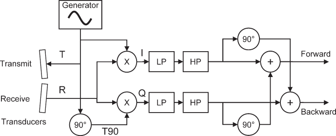
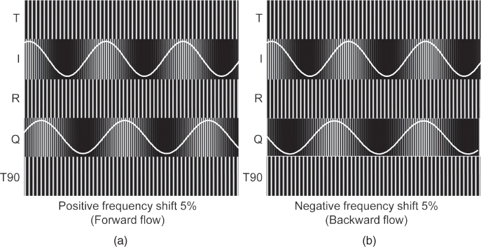
Figure 11.10 Demodulated I and Q signals for two received Doppler signals R shifted 5% up (a) and 5% down (b) in frequency by forward and backward flow, respectively. The overlaid sine shows the low frequency component, which is the demodulated Doppler signal after lowpass filtering. The phase shift of the Q component with respect to the I component is + 90° for the forward flow and − 90° for the backward flow. Signal names correspond to the figure above.
In practice, the Doppler signal of a blood vessel is not shifted to a single frequency but is a mixture of frequency shifts because blood flow varies over the cross section of the vessel. In addition, blood flow varies with the heart cycle. To determine the strength of the different frequency components, the Doppler signals are Fourier transformed in real time over short time intervals. The time varying frequency spectrum of the Doppler signal can be presented to the user as a brightness-coded image, as shown for pulsed Doppler measurements in Figure 11.12.
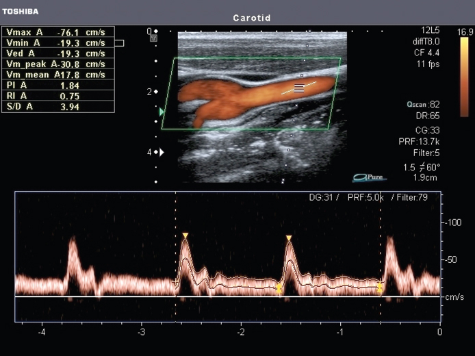
Figure 11.12 Pw-Doppler measurement and spectral Doppler representation. Blood flow is measured in the carotid close to the bifurcation. The red color overlay in the image is the color Doppler mode presentation. The direction of the measurement beam is represented by the dotted line in the image. The measurement window is marked by the two horizontal bars along the dotted line. In the vessel, angle direction measured by the user is presented by a further line. This allows presenting the data with the correct blood flow velocity. In the lower section, spectral Doppler measurements are overlaid with maximum and mean flow curves. Image courtesy of Toshiba Medical Systems.
11.3.1.2 Pulsed Wave Doppler
The disadvantage of cw-Doppler is the range ambiguity of the method: all vessels intersecting the interrogating beam contribute to the Doppler signal. To restrict the Doppler measurement to a certain depth, a gated measurement technique that uses pulsed sine bursts was introduced (Baker, 1970; Wells, 1969). For easier detection of the Doppler shift, pulses are longer than the imaging pulses and are sent interleaved with the image acquisition. However, Doppler shifts cannot be measured by the frequency shift of the spectrum of a single pulse: the pulse duration determines the frequency resolution of the Fourier transform of the pulse. Even with a long sine burst of 10 cycles at 1 MHz, the pulse duration is 10 μs and the achievable frequency resolution is the reciprocal, that is, 100 kHz. This is obviously insufficient to measure typical Doppler shifts of less than 15 kHz. Therefore, the pulse measurement has to be repeated several times with a fixed phase relation of the sine-burst pulses as depicted in Figure 11.11.
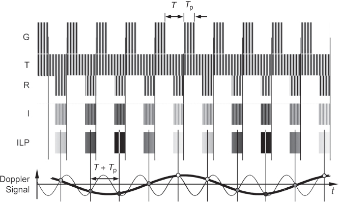
Figure 11.11 Pulse Doppler measurement: sine bursts G are sent with a fixed repetition time T + Tp, and the received echoes R are sampled after a fixed time delay corresponding to the measurement depth. The I signal is thus also gated, and after the lowpass filter, only a sampled version of the Doppler signal (thick line) is measured. Note that the second Doppler signal with a much higher frequency (thin line) has the same sample points, leading to velocity ambiguity if the repetition frequency is too low, that is, smaller than the double of the Doppler frequency.
The received signal is sampled at the time that corresponds to the desired measurement depth. Echoes from stationary objects will remain identical with each sampling, resulting in a constant signal. For a moving object, the phase of the returning sine wave will change. Ignoring propagation effects on the transmitted signal s, the received signal r from depth d will be (Jensen, 1996)
11.23 ![]()
which is a time-scaled version of the transmit pulse. In addition, the time delay τ between echo pulses is scaled relative to the time delay TPRF between transmit pulses according to
11.24 ![]()
This leads to a sampled signal slowly varying at the Doppler shift frequency. Again, as with cw-Doppler, quadrature demodulation can be used to detect the direction of flow. However, with Pulsed Wave Doppler (pw-Doppler), it is not realized by mixing with a phase-shifted reference signal but by sampling the echo signals a second time with a time delay corresponding to a 90° phase shift of the sine-burst frequency. For a detailed analysis of pw-Doppler, refer to the book by Jensen (1996).
In this technique, each pulse results only in a single sample point of the Doppler signal. Therefore, pw-Doppler is a sampling measurement of the Doppler signal that has to fulfill the sampling theorem: the sampling frequency, which is identical to the pulse repetition frequency, has to be twice as high as the frequency of the Doppler signal.
However, none of the two frequencies can be set freely by the user: The pulse repetition frequency depends on the depth of measurement. The closer the blood flow is to the transducer, the higher is the sampling frequency. Equation (11.20) shows the possibilities to lower the Doppler frequency shift for a given blood flow velocity: only the transmit frequency of the sine bursts can be lowered by the user. This is the reason why cardiac transducers use a lower frequency around 2 MHz at the cost of image resolution. However, the Doppler frequency shift may exceed half the pulse repetition rate, leading to aliasing and to the measurement of wrong Doppler shift frequencies and corresponding blood flow velocities. These situations have to be recognized by the clinical user.
11.3.1.3 Color Doppler Imaging and Power Doppler Imaging
Pw-Doppler measurements offer an exact assessment of blood flow velocity distributions over time in a single measurement window. However, often it is desired to get an overview of blood flow in a larger area such as in vessel bifurcations or in the heart. Unfortunately, it is not possible to quickly scan a pulsed Doppler measurement over an area of interest because pw-Doppler needs pulsing in the order of 100 times at one spot to calculate a Fourier transform. Scanning such a measurement would take too long and pose the risk of tissue heating. Therefore, by color Doppler imaging, only the average flow velocity is determined with fewer pulses and overlaid as a color-coded velocity image.
For this, similar to pw-Doppler, the echo signals are sampled at intervals TPRF for the in-phase component In and with a time shift of 90° of the transmit frequency for the quadrature Qn component. The most robust estimator (Evans, 1993) for the mean Doppler shift frequency can be calculated for N samples by the autocorrelator (Kasai et al., 1983):
The direction and mean frequency are color coded, typically in a red/blue color table. Some systems additionally calculate the variance of the velocity distribution and add a green color component to the color table if an increased variance is observed. This feature can be helpful in identifying turbulences in blood flow, which show large variances.
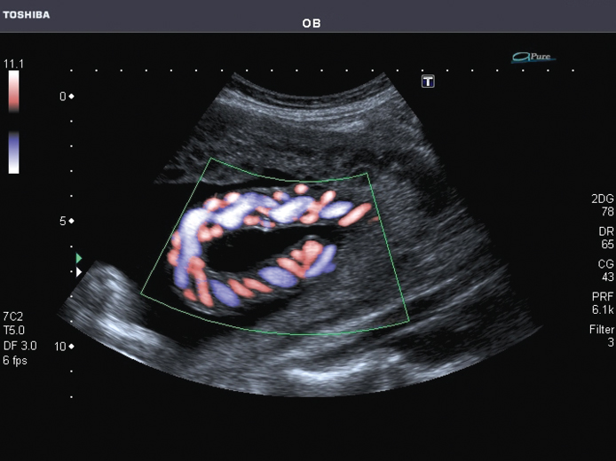
Color flow imaging also uses sampling of the Doppler signal and can show aliasing if the sampling frequency is too low for the measured flow velocities. Aliasing will show as a switch over from the end of the color scale to the beginning (e.g., from red to blue) and has to be differentiated from local turbulence that might also lead to a reversal of flow. Figure 11.13 shows an example of color flow imaging of the fetal umbilical cord.
Figure 11.13 Example of color flow imaging in the fetal umbilical cord. The two smaller arteries and the larger single vein can be seen clearly with their opposing blood flow direction. Note the missing signal for any blood flow directed orthogonal to the insonifying beam. Image courtesy of Toshiba Medical Systems.
Another variant of color Doppler imaging is power Doppler imaging (Rubin et al., 1994), in which only the average power of the sampled Doppler signal is presented, typically in a temperature color scale from red to yellow. It can also be calculated from the IQ components by
11.26 
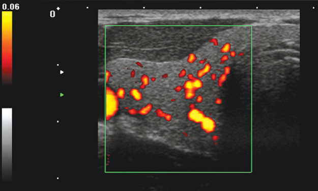
Although the signal is sampled, no aliasing problems occur because the power of the signal is calculated correctly even in the case of aliasing: total power is calculated by integration over the frequency spectrum of the signal. Owing to aliasing, signal components may be misplaced in the frequency domain, but the integral is not affected by this. Power Doppler shows neither the direction nor the velocity but only the existence of flow. Signals do not get stronger because of higher flow rates but because of stronger scattering of the flowing medium. Power Doppler is more sensitive than color Doppler and is used to show the presence of blood flow even in small vessels (Fig. 11.14).
Figure 11.14 Power Doppler imaging of the thyroid. Very small vessels that cannot be visualized by color Doppler can be found by power Doppler. However, only the presence of blood flow is visualized, neither the flow velocity nor its direction can be determined from the image. Image courtesy of Toshiba Medical Systems.
11.3.2 Ultrasound Contrast Agents and Nonlinear Imaging
11.3.2.1 Ultrasound Contrast Media
Scattering from blood is low compared to other tissues and makes blood flow difficult to image in small vessels. Gramiak and Shah (1968) were the first to use small gas bubbles to increase the echoes from blood. This led to the design of specific contrast agents consisting of gas microbubbles stabilized by a shell. It is obvious from the very low acoustic impedance of gases that microbubbles represent strong scatterers, and de Jong (1993) calculated that their scattering cross section is greater by a factor of 108 than that of an iron sphere of the same radius. In addition, gas microbubbles exhibit resonant and nonlinear properties that make them even stronger scatterers that can be sensitively detected by their nonlinear response.
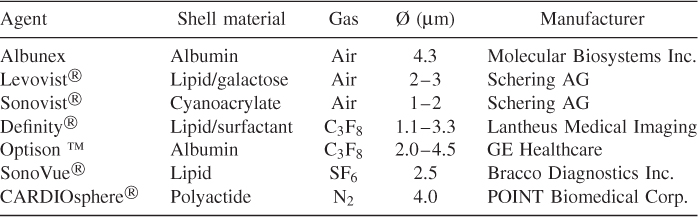
Table 11.2 lists some contrast agents. First-generation microbubbles (Albunex, Levovist) were air-filled and were filtered out quickly by the lung. Second-generation contrast agents (Definity, Sonovue, Optison) are filled with low solubility gases and are stable for several minutes. They are administered intravenously and can pass the lung. Polymer-shelled microbubbles such as Sonovist can live even longer and can be phagocytosed by the reticuloendothelial system and thus accumulate in the liver and spleen where they can last for several hours. Third-generation contrast agents (e.g., CARDIOSphere) aim at well-defined and reproducible bubble properties, such as constant shell thickness and a narrow radius distribution. Figure 11.15 shows a microscopic image of self-fabricated microbubbles with 5 μm average diameter with lipid shells filled with SF6.
Figure 11.15 Contrast microbubbles containing sulfur hexafluoride with a phospholipid shell (optical microscopy, experimental microbubbles from the author's laboratory).
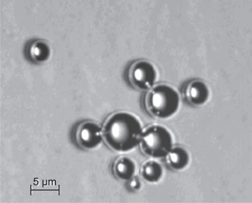
Table 11.2 Examples of Ultrasound Contrast Agents and Their Composition
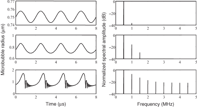
The oscillation of microbubbles in an ultrasound field is nonlinear; in the rarefaction phase the bubble expands and can reach several times its resting radius. However, in the compression phase, the bubble cannot be compressed as far. The motion equations for contrast media are nonlinear differential equations, such as the equation of Rayleigh, Plesset, Neppiras, Noltingk, and Poritsky (RPNNP equation) modified for the stiffness of the shell or a modified Herring equation (Doinikov and Dayton, 2006). Figure 11.16 shows the simulated radius change for a free gas bubble for different driving pressures. For low pressures, also called low MI imaging because of the low mechanical index, the bubble behaves like a linear resonator. For increasing pressures, the bubble behavior becomes more and more nonlinear. This leads to increasing deviations from the sinusoidal form of the driving pressure and generates harmonic frequencies in the spectrum of the scattered signal of the bubble (Schrope and Newhouse, 1993). This can be used for the sensitive detection of bubbles as discussed below. In this so-called medium MI range, the bubble shows stable nonlinear oscillation. Apart from the generation of harmonics, microbubbles can generate subharmonics and ultraharmonics (Shi et al., 1999, 2001), an effect typical for nonlinear dynamic systems close to chaotic behavior.
Figure 11.16 Simulated response of a microbubble with 0.75-μm resting radius and excitation at 500 kHz. For the panels on the left, the pressure increases from top to bottom, resulting in higher harmonics in the frequency representation in the panels on the right.
The strong mechanical activity of microbubbles can lead to tissue damage such as capillary rupture (Miller and Quddus, 2000). Therefore, guidelines for the safe use of contrast media have been issued (Albrecht et al., 2004).
Increasing the driving pressure even further to the high MI range leads to bubble destruction (Chomas et al., 2001; de Jong et al., 2002). Destruction takes place during the very fast compression of the bubble and typically fragments the bubble into smaller bubbles that dissolve (Chomas et al., 2001; Postema et al., 2004). This effect is used in imaging protocols for destruction of contrast agents and the quantification of subsequent replenishment to assess tissue perfusion. When collapsing, the microbubbles emit a broadband signal that can be detected and is known as Stimulated Acoustic Emission (SAE). The disappearance of the microbubble leads also to a loss of correlation and thus to a strong short Doppler signal (Tiemann et al., 2000), which can also be used for microbubble detection.
11.3.2.2 Harmonic Imaging Techniques
The first method to detect the harmonic response from microbubbles was to use bandpass filters for the second harmonic (Schrope and Newhouse, 1993). This technique has several disadvantages: the broadband spectrum of an imaging pulse shows considerable overlap with the second harmonic and the pulse spectrum as well as the second harmonic must fit in the limited bandwidth of transducers. To better understand the generation of harmonics, the nonlinear response of the microbubbles can be modeled by a nonlinear system with memory by a Volterra series (Mleczko et al., 2009) when sub- and ultraharmonics are neglected.
where the kernels hi characterize the behavior of the nonlinear system for an input signal x(t) and output signal y(t). For a sinusoidal input signal of frequency f0, the linear term with kernel h1 generates only the original frequency f0. The term with the quadratic kernel generates a constant output at frequency zero and a component at 2f0. The cubic term with kernel h3 generates components at f0 and 3f0. In general, the even kernels of order n generate a constant signal and all even multiples of f0 up to nf0. The odd order kernels of order n generate all odd multiples of f0 up to nf0. All odd order terms generate a component with the original transmit frequency that can be sensitively detected by the transducer.
To overcome the disadvantages of harmonic imaging by filtering the second harmonic, at the moment two different techniques are used, which send two or three pulses. The basic idea behind both schemes is that linear signal components cancel when the echoes of the pulses are added.
The first technique is Pulse Inversion (PI) imaging (Hope Simpson et al., 1999). Here, two pulses with opposite signs are transmitted in two transmit/receive cycles. When the received echoes are modeled according to Eq. (11.27), it can be seen that the addition of the two echo signals cancels all odd order components, including the linear term. The even order terms are still present in the sum signal, and the lowest frequency component is 2f0. This component will be the only one with a significant contribution to the received signal because of the bandpass character of the transducer and the lowpass characteristic of tissue attenuation. A disadvantage of this method is that higher odd order terms are cancelled, although they could contribute to signal energy around f0 (Fig. 11.17).
Figure 11.17 Pulse inversion contrast image (b) of a tissue mimicking phantom with a circular inclusion filled with contrast medium in water compared to the B-mode image without pulse inversion (a).
Therefore, another pulsing scheme was proposed (Phillips, 2001) with three pulses (Contrast Pulse Sequencing, CPS), with the relative amplitudes − 1/2, 1, − 1/2 for the three pulses. Again, the echoes cancel the linear term for the three echoes according to Eq. (11.27). However, components with higher order still contribute to the sum signal, irrespective of even or odd order. Since the odd order components generate contributions at the fundamental frequency, the method gives higher amplitudes for the harmonic signal.
In addition, subharmonics and ultraharmonics can be used for better differentiation between tissue and microbubble nonlinearities because they are unique to microbubbles (Chomas et al., 2002).
11.3.2.3 Perfusion Imaging Techniques
To measure tissue perfusion, that is, the blood supply to capillary vessels in the tissue, different approaches exist.
Wei et al., (1998) introduced a technique known as destruction–reperfusion or replenishment, later successfully used for the assessment of myocardial perfusion (Tiemann et al., 1999). They proposed a constant venous infusion with contrast agent. Then, after an equilibrium concentration of the contrast agent in tissue is reached, a high MI burst pulse is used to destroy all microbubbles in the imaging plane. Subsequently, the amount of the inflow of new microbubbles is observed with low MI imaging pulses after varying delays. With this method, it has to be taken into account that the imaging pulse itself may also destroy microbubbles. Thus, for each delay, a new destruction–reperfusion experiment has to be performed. Therefore, this measurement technique is time consuming.
A less time-consuming alternative to the replenishment technique is the depletion method (Eyding et al., 2003), which uses the imaging pulses to destroy a certain percentage of contrast microbubbles. Again, at the beginning, a constant perfusion with contrast agent is realized by intravenous infusion. It can be shown that an exponential decay can be observed with a fast sequence of semidestructive imaging pulses. Using mathematical models, perfusion can be calculated from the measurements by fitting of the model parameters.
The fastest way to find perfusion parameters is the bolus method (Eyding et al., 2002): one bolus of contrast microbubbles is administered and flows into the imaging plane with a time delay. Several parameters can be calculated from time–intensity curves in the imaging plane that are imaged by nondestructive pulses: peak intensity, time to peak, and peak width. Especially, time to peak has shown good correlation with perfusion quantification with Nuclear Magnetic Resonance (NMR) imaging (Meves et al., 2002, Chapter 5). Techniques for quantification of perfusion are still under development and have to be adapted to the specific application and contrast agent.
Another method to quantify contrast microbubbles in the capillaries is the detection of SAE or loss of correlation. Up to microbubble concentrations of 15,000 bubbles per milliliter, a linear relationship of the square root of the Doppler signal intensity could be demonstrated (Tiemann et al., 2000). At higher concentrations, the acoustic attenuation of microbubbles close to the transducer hinders the destruction of deeper ones, thus rendering quantitative measurements impossible. Therefore, Sensitive Particle Acoustic Quantification (SPAQ) has been proposed to quantify higher microbubble concentrations (Reinhardt et al., 2005). With this method, the volume of interest is slowly scanned by a lateral transducer movement in steps of 10–100 μm, so that only a few microbubbles have to be destroyed after one motion step. This technique allows quantification of higher concentrations (30,000 bubbles/mL), but has not been realized in real time so far.
11.3.2.4 Targeted Imaging
Advances in molecular biology drive the demand for imaging techniques that can show the presence or absence of molecules that are connected with certain disease states, especially in oncology and cardiovascular applications. For this application field, named molecular imaging, the sensitivity of the imaging method for small amounts of the target molecule is crucial for success. So far, nuclear imaging with Positron Emission Tomography (PET, Chapter 7) is the only modality that is clinically established for molecular imaging and has the highest sensitivity. However, for molecules expressed by vascular endothelial cells, ultrasound molecular imaging also shows promising results in preclinical studies (Bloch et al., 2004; Dayton and Ferrara, 2002; Lindner, 2004).
In principle, two different mechanisms are used to bind microbubbles to the target cells: in so-called passive targeting, either the chemical composition of the microbubble shell is responsible for binding or ligands binding to the targeted molecule are attached to the bubble surface. The main application field is better diagnosis of inflammation, thrombus, and angiogenesis.
Passive targeting of Albunex microbubbles was described by Wei et al., (2001) for myocardial inflammation. Activated leukocytes cling to albumin in the shell of the microbubbles and thus transport them to the inflammation. A similar effect was also used for imaging myocardial inflammation in dogs in vivo with passive targeting caused by phosphatidyl serine as part of the lipid composition of the microbubble shell (Christiansen et al., 2002), showing high sensitivity comparable to radionuclide imaging.
Active targeting has been demonstrated by, Weller et al., (2003) and Villanueva et al., (2007), with ICAM-1 (intracellular adhesion molecule) and selectins as target molecules expressed during inflammation. The study by Villanueva et al., (2007) showed the possibility of diagnosing a recent ischemia event by such methods.
Quantification in these applications is currently realized by the following imaging protocol: after bolus injection of the targeted contrast media, an image is taken after a delay to record the concentration of bound and unbound microbubbles in the tissue. Then, a destructive ultrasound pulse clears all microbubbles, and after a shorter delay, a second image records only unbound microbubbles. Subtraction of the intensity of both frames results in a quantitative measure of targeted microbubble concentration.
The second application field, thrombus imaging, has been addressed using microbubbles targeted to GPIIb/IIa, a glycoprotein overexpressed in thrombi. For example, with quantitative techniques, a significant increase in microbubble concentration in thrombi could be shown (Alonso et al., 2007).
Especially in the detection of cancer, markers of angiogenesis are of interest, such as αvβ3 (Ellegala et al., 2003), α5β1 (Leong-Poi et al., 2005), or VEGFR2 (vascular endothelial growth factor receptor). Apart from cancer diagnosis, quantitative molecular imaging techniques for angiogenesis can be used to monitor the effect of antiangiogenic drugs in cancer therapy. The development of ultrasound molecular imaging techniques is currently a constantly growing application field.
11.4 Application Examples of Biomedical Sonography
11.4.1 B-Mode, M-Mode, and 3D Imaging
The standard imaging mode of ultrasound scanners is the B-scan or B-mode image relying on the pulse-echo imaging principle. In current systems, it is typically electronically scanned with transducer arrays and the beamforming techniques described earlier. Depending on the transducer, the resolution of these images is in the range from 0.1 to 3 mm. Figure 11.18 shows an example of B-mode imaging of a fetus with a convex array. The dots show a centimeter scale. Often, arrows on the depth scale mark the position of one or more transmit foci; in the image, one transmit focus at 5-cm depth was used. The frequency of the array was chosen in the range from 3 to 10 MHz because with the total image depth of 9 cm, maximum attenuation is still low enough to use this frequency range. This results in an axial resolution in the direction of the soundbeam below 1 mm and lateral resolution in the range of 1 mm at the focal depth of 5 cm. In the image, several artifacts of ultrasound imaging can be observed: surfaces give a stronger echo signal if the incidence is at 90°. This can be seen at the tip of the nose showing a bright spot in the position where it is insonified perpendicular to the surface. Furthermore, acoustic shadowing by the strong reflection and absorption of bone structures inside the head can be seen leading to missing echo signals at 4 cm behind the nose. However, imaging the brain through the skull bone is no problem in fetal imaging, because the fetal skull is still acoustically transparent.
Figure 11.18 B-mode image of fetal profile showing minute details of brain and thorax. A convex array with a bandwidth from 3 to 10 MHz was used. The electronic transmit focus is at 5 cm depth, as indicated by the arrow on the left. In receive mode, dynamic focusing moves the focus continually to the depth of echo origin. Image courtesy of Toshiba Medical Systems.
By mechanically moving the array in a direction perpendicular to the electronic scan direction, 3D images can be acquired. This can also be achieved by electronic beamforming with a two-dimensional array as discussed earlier. If imaging is fast enough or synchronized with the Electrocardiogram (ECG) signal, volume images of the moving heart can be acquired.
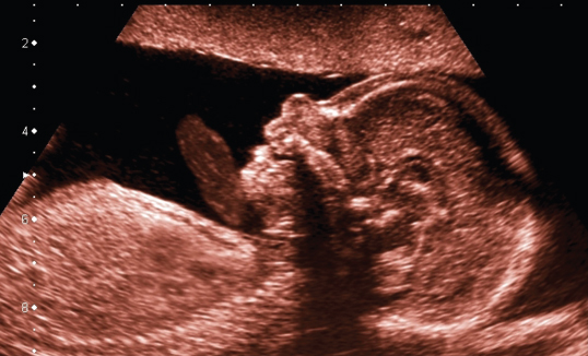
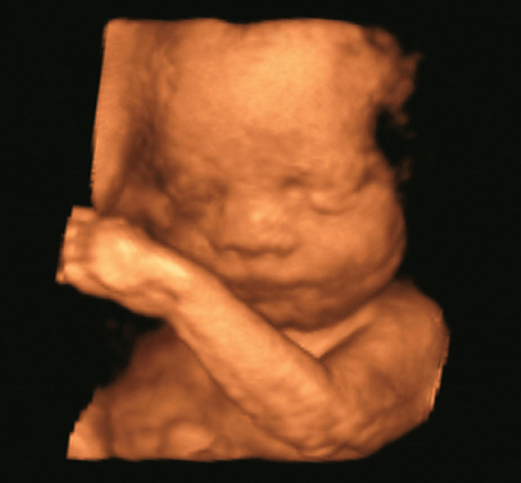
However, the most popular three-dimensional images are fetal faces, as shown in Figure 11.19. This image is a snapshot of a movie that was taken with a fast mechanical scan of a one-dimensional array resulting in real-time images of the moving fetus. In both applications, cardiac imaging and fetal imaging, 3D rendering is easier than in other applications because the contrast between the low echo level from blood or amniotic fluid and the high echo level from tissue allows good surface detection.
Figure 11.19 Three-dimensional rendering of fetal face and arm. The image is a snapshot of a movie sequence recorded with a mechanically scanned convex array with 2- to 7-MHz bandwidth. Image courtesy of Toshiba Medical Systems.
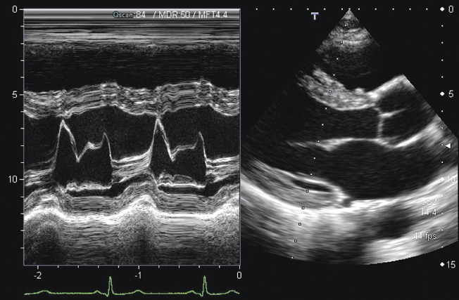
For cardiac imaging, it is often of interest to study the motion of the valves or the myocardium over the heart cycle. To facilitate this, ultrasound scanners offer the M-mode (motion mode, sometimes also called TM-mode for time-motion mode). In this mode, one line along a fixed position is measured continuously and presented as in B-mode with brightness-coded intensity. The temporal changes of echo signals are shown by plotting one line next to the other in a moving window, similar to an ECG signal. This is shown in Figure 11.20 on the left. Therefore, the horizontal scale is a time scale. On the right side, a typical B-mode image of the heart can be seen. For cardiac imaging often phased arrays are used, which scan the image only by steering the beam. This leads to a sector image with all scan lines originating at one point in the middle of a relatively small transducer. This is due to the small windows between the ribs that have to be used to get acoustic access to the heart. The B-mode image is used to determine the position of the M-mode measurements, indicated in the right image by the dotted line.
Figure 11.20 B-mode sector scan image of the adult heart (right), with the dotted line marking the measurement position for the M-mode image presented on the left. The vertical scale in the M-mode is in centimeters; the horizontal scale is in seconds. The continuously measured A-scan line cuts through the mitral valve. The strong movement of the valve over a period of 2 s can be observed clearly and can be related to the ECG signal shown in green at the bottom. Image courtesy of Toshiba Medical Systems.
11.4.2 Flow and Perfusion Imaging
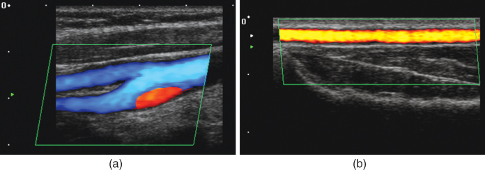
Functional imaging of flow and perfusion is a particular strength of ultrasound imaging. Examples have already been presented and discussed in the sections on Doppler and perfusion measurement techniques, and this section gives further examples for the most important applications. In vascular imaging, flow can either be assessed quantitatively with color Doppler imaging or just be detected, to demonstrate organ perfusion or patency of vessels. Figure 11.21 shows examples for both modes. In Figure 11.21a, color Doppler is used to image the carotid bifurcation with blood flow going from right to left. Owing to the bifurcation, turbulence is induced and leads to a backflow of blood, which is shown in red. A much lower blood flow speed is seen in the radial artery on the right side (Fig. 11.21b) and is detected with power Doppler imaging. In both images, the green parallelogram indicates the measurement area, which is restricted to speed up imaging and can be placed in the image by the user. The images also show the excellent resolution that can be achieved with today's ultrasound scanners. In both cases, the arteries are close to the skin surface and image depth is 3 and 2 cm, respectively. Therefore, high frequency arrays can be used. For the image in Figure 11.21a, 11.21a 6- to 11-MHz bandwidth transducer and that in Figure 11.21b, an 8- to 14-MHz transducer were used to image the radial artery of 3 mm diameter.
Figure 11.21 (a) Color Doppler flow measurement of the carotid bifurcation. The blue color codes flow with a component away from the transducer (down to the left). A reverse flow due to turbulence is visible as a red signal. Image depth is 3 cm, and a linear array with 6- to 11-MHz bandwidth was used. (b) Power Doppler image of flow in the radial artery. Image depth is only 2 cm, and a high frequency transducer array with 8- to 14-MHz bandwidth was used. Image courtesy of Toshiba Medical Systems.
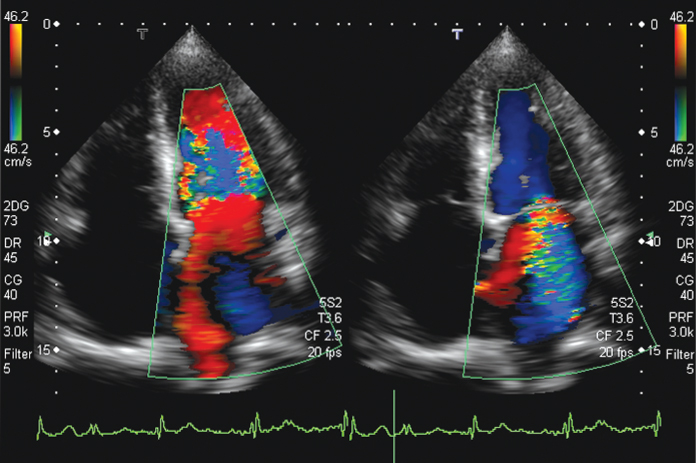
A main application of color Doppler imaging is blood flow measurement in the heart. For this, phased array transducers are used and center frequencies are chosen around 2–3 MHz to avoid aliasing in the Doppler signals: according to Eq. (11.20), the Doppler shift frequency is proportional to the center frequency of the pulse and to the blood flow speed. At the same time, the measurement depth has to reach up to 15 cm, as can be seen in Figure 11.22, which determines the maximum Pulse Repetition Frequency (PRF) (1540 ms−1/0.3 m = 5.1 kHz). In Figure 11.22, an even lower PRF of 3 kHz was used, allowing a maximum Doppler shift frequency of 1.5 kHz to avoid aliasing. The center frequency chosen was 2.5 MHz. With Eq. (11.20), the maximum speed that can be measured can be calculated using the maximum Doppler shift:
11.28 ![]()
This is also indicated by the velocity scale on the color bar at the side of Figure 11.22. The color Doppler processing relies on a certain number N of consecutive pulses with the PRF. The mean Doppler frequency is calculated according to Eq. (11.25). In addition, the variance of subsequent measurements can be analyzed and gives for large values an indication that flow may be turbulent. This is used in some systems to change the color scale if turbulent flow is assumed. This is also shown in Figure 11.22: an additional green-yellow color scale is used for turbulent flow, which is, for example, present in the high speed jet on the right side of the figure.
Figure 11.22 Color-coded blood flow in the heart. Flow to the transducer (to the top) is shown in red; flow in the downward direction is blue. In addition, turbulence is detected and color coded by a green/yellow overlay. Left: inflow of blood into the left ventricle through the open mitral valve (shown in red). Turbulent flow with downward components or aliasing occurs in the left ventricle. Right: the mitral valve is closed; however, a high speed leakage jet shown in blue, with turbulent components in green, can be seen and demonstrates malfunction of the valve. Blue color in the ventricle shows outflowing blood through the aortic valve. Images were recorded with a phased array with 2- to 5-MHz bandwidth and 2.5-MHz center frequency. Image courtesy of Toshiba Medical Systems.
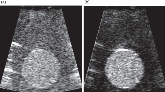
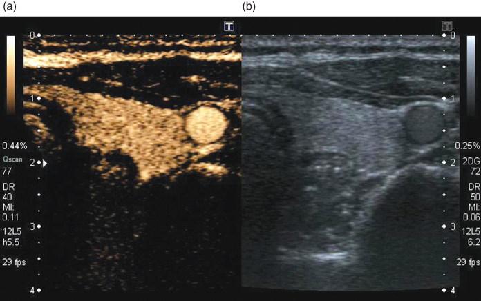
Low perfusion is better imaged with the use of contrast media as described earlier. In Figure 11.23, an example of a contrast study of thyroid perfusion is shown. In the normal thyroid, the perfusion is homogeneous, and the good contrast to tissue ratio of PI imaging at low MI can be seen on the left in comparison to the normal B-mode image on the right. The carotid artery clearly shows the strong contrast increase of blood relative to the B-mode image. The suppression of the linear signals from normal tissue is demonstrated by the low intensity of muscle tissue in front of the thyroid. Clinically, further applications for ultrasound contrast media are, for example, perfusion measurements of the liver to detect focal liver disease or brain perfusion imaging for stroke detection. Perfusion imaging techniques are under continuous development and can be expected to be extended by applications of targeted imaging in the future.
Figure 11.23 Simultaneous real-time display of normal thyroid in B-mode (b) and low MI pulse subtraction contrast harmonic imaging (a). Homogeneous uptake of microbubbles in the left lobe of the thyroid and microbubbles in the carotid artery can be seen. The MI of the imaging modes is 0.11 for the harmonic imaging mode and 0.06 for the normal B-mode image. Image courtesy of Toshiba Medical Systems.
Albrecht T, Blomley M, Bolondi L, Claudon M, Correas J-M, Cosgrove D, Greiner L, Jäger K, de Jong N, Leen E, Lencioni R, Lindsell D, Martegani A, Solbiati L, Thorelius L, Tranquart F, Weskott H P, Whittingham T. Guidelines for the use of contrast agents in ultrasound. Ultraschall Med 2004;25:249–256.
Alonso A, Della Martina A, Stroick M, Fatar M, Griebe M, Pochon S, Schneider M, Hennerici M, Allemann E, Meairs S. Molecular imaging of human thrombus with novel abciximab immunobubbles and ultrasound. Stroke 2007;38(5):1508–1514.
Baker DW. Pulsed ultrasonic blood-flow sensing. IEEE Trans Son Ultrason 1970;SU-17:170–185.
Bamber JC. Ultrasonic properties of tissue. In: Duck FA, Baker AC, Starrit HC, editors. Ultrasound in Medicine. Bristol: Institute of Physics Publishing; 1998.
Bloch SH, Dayton PA, Ferrara KW. Targeted imaging using ultrasound contrast agents. IEEE Eng Med Biol Mag 2004;23:18–29.
Chomas JE, Dayton P, Allen J, Morgan K, Ferrara KW. Mechanisms of contrast agent destruction. IEEE Trans Ultrason Ferroelectr Freq Control 2001;48(1):232–248.
Chomas J, Dayton P, May D, Ferrara K. Nondestructive subharmonic imaging. IEEE Trans Ultrason Ferroelectr Freq Control 2002;49(7):883–892.
Christiansen JP, Leong-Poi H, Klibanov AL, Kaul S, Lindner JR. Non-invasive imaging of myocardial reperfusion injury using leukocyte-targeted contrast echocardiography. Circulation 2002;105:1764–1767.
Dayton PA, Ferrara KW. Targeted imaging using ultrasound. J Magn Reson Imaging 2002;16:362–377.
Doinikov AA, Dayton PA. Spatio-temporal dynamics of an encapsulated gas bubble in an ultrasound field. J Acoust Soc Am 2006;120(2):661–669.
Duck FA. Physical Properties of Tissue. New York: Academic Press; 1990.
Ellegala D, Leong-Poi H, Carpenter JE, Klibanov AL, Kaul S, Shaffrey ME, Sklenar J, Lindner JR. Imaging tumor angiogenesis with contrast ultrasound and microbubbles targeted to αvβ3. Circulation 2003;108:336–341.
Evans DH. In: Wells PNT, editor. Advances in Ultrasound Techniques and Instrumentation. New York: Churchill Livingstone; 1993. Chapter 8.
Eyding J, Wilkening WG, Postert T. Brain perfusion and ultrasonic imaging techniques. Eur J Ultrasound 2002;16:91–104.
Eyding J, Wilkening WG, Reckhardt M, Schmid G, Meves SH, Ermert H, Przuntek H, Postert T. Contrast burst depletion imaging (CODIM): a new imaging procedure and analysis method for semiquantitative ultrasonic perfusion imaging. Stroke 2003;34:77–83.
Gramiak R, Shah PM. Echocardiography of the aortic root. Invest Radiol 1968;3:356–366.
Hickling R. Analysis of echoes from a solid elastic sphere in water. J Acoust Soc Am 1962;34:1582–1592.
Hope Simpson D, Chin CT, Burns PN. Pulse inversion Doppler: a new method for detecting nonlinear echoes from microbubble contrast agents. IEEE Trans Ultrason Ferroelectr Freq Control 1999;46(2):372–382.
Jensen JA. A model for the propagation and scattering of ultrasound in tissue. J Acoust Soc Am 1991;89(1):182–190.
Jensen JA. Estimation of Blood Flow Velocities Using Ultrasound. Cambridge: Cambridge University Press; 1996.
de Jong N. Acoustic properties of ultrasound contrast agents [PhD thesis]. Erasmus University Rotterdam: 1993.
de Jong N, Bouakaz A, Frinking P. Basic acoustic properties of microbubbles. Echocardiography 2002;19(3):229–240.
Kasai C, Namekawa K, Koyano A, Omoto R. Real-time two dimensional blood flow imaging using an autocorrelation technique. IEEE Trans Son Ultrason 1983;SU-32:458–464.
Leong-Poi H, Christiansen J, Heppner P, Lewis CW, Klibanov AL, Kaul S, Lindner JR. Assessment of endogenous and therapeutic arteriogenesis by contrast ultrasound molecular imaging of integrin expression. Circulation 2005;111(24):3248–3254.
Lindner JR. Microbubbles in medical imaging: current applications and future directions. Nat Rev: Drug Discov 2004;3:527–532.
Meves SH, Wilkening WG, Thies T, Eyding J, Finger THM, Schid G, Ermert H, Postert T. Comparison between echo contrast agent-specific imaging modes and perfusion weighted magnetic resonance imaging for the assessment of brain perfusion. Stroke 2002;33:2433–2437.
Miller DL, Quddus J. Diagnostic ultrasound activation of contrast agent gas bodies induces capillary rupture in mice. Proc Natl Acad Sci U S A 2000;97(18):10179–10184.
Mleczko M, Postema M, Schmitz G. Discussion of the Application of Finite Volterra Series for the Modeling of the Oscillation Behaviour of Ultrasound Contrast Agents. Applied Acoustics. 2009;70(10):1363–1369.
Morse PM, Ingard KU. Theoretical Acoustics. New York: McGraw-Hill; 1968.
Phillips P. Contrast pulse sequences (CPS): imaging nonlinear microbubbles. Proc IEEE Ultrason Symp 2001;2:1739–1745.
Postema M, van Wamel A, Lancée CT, de Jong N. Ultrasound-induced encapsulated microbubble phenomena. Ultrasound Med Biol 2004;30(6):827–840.
Reinhardt M, Hauff P, Briel A, Uhlendorf V, Linker RA, Mäurer M, Schirner M. Sensitive particle acoustic quantification (SPAQ): a new ultrasound-based approach for the quantification of ultrasound contrast media in high concentrations. Invest Radiol 2005;40(1):2–7.
Rubin JM, Bude RO, Carson PL, Bree RL, Adler RS. Power Doppler ultrasound: a potential useful alternative to mean-frequency-based color Doppler ultrasound. Radiology 1994;190:853–856.
Schmitz G. Ultrasound in medical diagnosis. In: Pike R, Sabatier P, editors. Scattering, Scattering and Inverse Scattering in Pure and Applied Physics. London: Academic Press; 2002. pp. 161–174.
Schrope BA, Newhouse VL. Second harmonic ultrasonic blood perfusion measurement. Ultrasound Med Biol 1993;19(7):567–579.
Shi WT, Forsberg F, Hall AL, Chiao RY, Liu J, Miller S, Thomenius KE, Wheatley MA, Goldberg BB. Subharmonic imaging with microbubble contrast agents: initial results. Ultrason Imaging 1999;21:79–94.
Shi WT, Forsberg F, Goldberg BB. Subharmonic imaging with contrast microbubbles. In: Goldberg BB, Raichlen JS, Forsberg F, editors. Ultrasound Contrast Agents: Basic Principles and Clinical Applications. London: Martin Dunitz Ltd; 2001. pp. 47–57.
Shung KK, Thieme GA. Ultrasonic Scattering by Biological Tissues. Boca Raton (FL): CRC Press; 1993.
Tiemann K, Lohmeier S, Kuntz S, Köster J, Pohl C, Burns PN, Porter TR, Nanda NC, Lüderitz B, Becher H. Real-time contrast echo assessment of myocardial perfusion at low emission power: first experimental and clinical results using power pulse inversion imaging. Echocardiogr J Cardiovasc Ultrasound Allied Tech 1999;16:799–809.
Tiemann K, Pohl C Schlosser T, Goenechea J, Bruce M, Veltmann C, Kuntz S, Bangard M, Becher H. Stimulated acoustic emission: pseudo-Doppler shifts seen during the destruction of nonmoving microbubbles. Ultrasound Med Biol 2000;26(7):1161.
Villanueva FS, Lu E, Bowry S, Kilic S, Tom E, Wang J, Gretton J, Pacella JJ, Wagner WR. Myocardial ischemic memory imaging with molecular echocardiography. Circulation 2007;115(3):345–352.
Wei K, Jayaweera AR, Firoozan S, Linka A, Skyba DM, Kaul S. Quantification of myocardial blood flow with ultrasound-induced destruction of microbubbles administered as a constant venous infusion. Circulation 1998;97:473–483.
Wei K, Ragosta M, Thorpe J, Coggins M, Moos S, Kaul S. Noninvasive quantification of coronary blood flow reserve in humans using myocardial contrast echocardiography. Circulation 2001;103(21):2560–2565.
Weller GER, Lu E, Csikari MM, Klibanov AL, Fischer D, Wagner WR, Villanueva FS. Ultrasound imaging of acute cardiac transplant rejection with microbubbles targeted to intercellular adhesion molecule-1. Circulation 2003;108(2):218–224.
Wells PNT. A range gated Doppler system. Med Biol Eng 1969;7:641–652.
Wild JJ. The use of ultrasound pulses for the measurement of biological tissues and the detection of tissue density changes. Surgery 1950;27:183–188.