
Chapter 2
Evaluation of Tomographic Data
2.1 Introduction
Through the last decades tomographic techniques have gained an ever-increasing importance in biomedical imaging. The great benefit of these techniques is the ability to assess noninvasively (and nondestructively) the three-dimensional structure of the investigated objects.
With regards to biomedical applications, several, but not all, available tomographic techniques allow the investigation of dynamic processes (e.g., transport phenomena) and repeated measurements in a single organism. One thus can differentiate between these in vivo techniques and in vitro techniques, which are suitable, for example, for investigations of tissue samples. Electron tomography (Chapter 6) belongs to the latter group. X-ray Computed Tomography (CT, Chapter 4), Magnetic Resonance Imaging (MRI, Chapter 5), as well as Single Photon Emission Computed Tomography and Positron Emission Tomography (SPECT and PET, Chapter 7) are generally (SPECT and PET exclusively) used for the noninvasive 3D imaging of living organisms. The aforementioned techniques are well suited to generate three-dimensional tomographic image volumes even of complete organisms such as the human body.
This contrasts with more recent developments in the area of optical imaging such as Optical Coherence Tomography (OCT), which utilize light sources within or near the visible range. Owing to the usually high absorption and scattering of light in tissue, the application of optical tomographic methods is generally restricted to investigation of near-surface structures such as the skin or the eye.
This chapter provides a rather general outline of the principal problems that one faces when evaluating tomographic data, with focus on the analysis of the image data. The important but highly specialized field of tomographic image reconstruction will be discussed only very shortly. The four tomographic in vivo techniques that currently are of relevance not only in basic research but also in clinical routine are as follows.
As already indicated, the different methods probe different properties of the living organisms investigated:
All tomographic techniques share, to a varying degree, the following characteristics:
Formally, evaluation of the tomographic data can be pursued along two different approaches.
On the one hand, tomographic data are, first and foremost, three-dimensional image data that provide information concerning the regional variation of the parameter producing the signal. Depending on the tomographic method used and on the experimental setting, it might not be possible (or necessary) to evaluate the data beyond visual inspection. This is, for instance, true if one is aiming solely at getting qualitative structural/anatomical information (e.g., investigating bone structures with X-ray CT).
In such a situation, methods for optimal image display, digital image processing, and especially tools for efficient 3D image data visualization such as volume rendering are of primary interest.
On the other hand, tomographic data frequently are valuable also in the sense that the image-generating signal is itself of interest as a quantitative measure. For example: while CT data are more often than not evaluated in a qualitative fashion, it is also possible to use the measured attenuation of the X-ray radiation to derive quantitative information concerning bone density. Some tomographic methods are more “quantitative” than others in the sense that they provide an image signal that is related in a better known way to the quantity of interest. Most desirable is the situation where the image signal is simply proportional to such a quantity, which allows, for example, direct interpretation of all image contrasts in terms of that quantity.
Probably the best example for this is the PET method. Here, the images represent quantitatively the number of radioactive decays of the applied tracer in the respective image pixel. Since this number in turn is directly proportional to the amount of tracer substance in the corresponding pixel volume, one obtains a direct measure of this quantity. PET images are therefore directly interpretable as quantitative tracer concentration maps.
For other modalities the situation usually is a bit more complicated. Taking MRI as an example, the images provide detailed information especially concerning the soft tissue anatomy, but it is rather difficult to derive reliable quantitative information such as concentrations of systemic substances. If contrast agents are applied, which is in a way the analogue of the tracers used in PET, although the applied amounts are larger by a factor of 106 or so in the case of MRI, one usually is not at all able to deduce the local contrast agent concentration quantitatively. This difficulty has its origin in the fact that the relationship between the concentration of the contrast agent and the contrast-agent-induced changes of the image signal is influenced by a number of factors whose precise effect cannot be quantified accurately. Therefore, the MRI image signal usually cannot be translated into truly quantitative measures of concentrations.
The discussion of the different quantitative capabilities of the above-mentioned different methods refers to the primary images that are delivered by the respective method. In doing so, one further important parameter that could be used has been ignored, namely, investigation of time-dependent processes by so-called dynamic investigations (in contrast to static “snapshot”-like studies).
Dynamic tomography requires the ability to perform the measurements for a single tomographic data set so fast that a sufficiently large number of such measurements can be performed over the interesting time window of the investigated process.
Depending on the method used, different factors limit the obtainable temporal resolution that typically goes down to the order of seconds in the case of CT, MRI, or PET.
2.2 Image Reconstruction
The basic idea of most tomographic approaches is to acquire two-dimensional projection images from various directions around the object of interest. It is necessary that the radiation, which directly or indirectly generates each image (X-rays, electron rays, γ-radiation, rf fields, etc.), is penetrating in the sense that each two-dimensional image can be seen as a projection of the real three-dimensional object onto the image plane1. The most straightforward example might be X-ray CT, where each projection is the same as a standard X-ray image acquired under that orientation.
Having acquired the projection data for a sufficiently complete set of directions, usually covering an angular range of 360° or 180° around the patient, the next step is tomographic image reconstruction.
Various standard mathematical techniques exist to calculate from a sufficiently complete set of projections the complete three-dimensional structure of the investigated object.
The algorithms can be roughly divided into two groups: analytical and iterative procedures.
The analytical procedures utilize variants of the filtered backprojection approach. This approach is based on a mathematical theorem that goes back to 1911, namely, the Radon transformation, which in two dimensions defines the relationship between the complete set of all possible line integrals (the projections or Radon transform) through a two-dimensional function f(x, y) and that function itself (which represents a cross-sectional slice through our object).
Iterative image reconstruction utilizes well-defined trial-and-error approaches whose background lies in mathematical statistics. Here, image reconstruction consists in providing the algorithm with an initial guess of the object that then is subjected to a simulated imaging process, thus generating artificial projection data that are compared with the actual measured data. From this comparison, correction factors are derived, which in turn are applied to each image pixel of the first image estimate, thus generating a new improved image estimate. This iterative loop of image estimation, simulated projection and image estimate improvement, is repeated until some convergence criterion is met.
Analytical image reconstruction is applied whenever the nature of the data allows it since the computational burden is much smaller than is the case for the iterative approaches. Analytical reconstruction is the default approach in CT as well as in MRI.
For SPECT and PET applicability of analytic procedures is limited. This is due to the fact that these tracer techniques operate at extremely high sensitivities (compared to CT and MRI) but suffer from influences of the statistical nature of the decay of the radioactive tracers, which translates into considerable statistical noise of the projection data. This in turn frequently leads to sizable artifacts during image reconstruction. In recent years, the ever-increasing computer speed allowed to move to iterative algorithms as the default reconstruction method in SPECT and PET.
2.3 Image Data Representation: Pixel Size and Image Resolution
The early tomographs usually acquired only single cross-sectional slices of an appreciable slice thickness (that is, low spatial resolution perpendicular to the primary image plane). Nowadays, tomographic techniques are capable of producing not only single cross-sectional images but, rather, contiguous stacks of such images representing consecutive cross-sections through the investigated object. The spatial orientation of the cross sections (i.e., image plane orientation) is usually determined by the orientation of the object within the Field of View (FOV) of the tomograph: with the exception of MRI the major techniques generate cross sections whose orientation is collinear to the symmetry axis of the tomograph's gantry, that is, the image plane is parallel to the plane defined by the tomograph's gantry. This slice orientation is usually called transaxial.
Despite the fact that the transaxial image plane is usually the one that has been measured in the first place, it is now primarily a matter of taste, whether one prefers to view data organized as a stack of consecutive two-dimensional transaxial images or as representing a three-dimensional digital image volume, which then can be “sliced” via suitable software tools to yield cross sections of arbitrary orientation.
The latter approach (arbitrary slicing of 3D volumes) only works well if the spatial resolution is similar along each direction within the image volume. This is guaranteed in modern designs where spatial resolution is indeed approximately isotropic.
From a user point of view, a tomograph can be then seen as a kind of 3D digital camera. As is the case for any digital camera, one has to be careful not to confuse actual image resolution with the digital grid on which the data are displayed. This point is at the same time trivial and a source of recurring confusion and will, therefore, be now examined more closely.
It is common usage to specify the number of image pixels along both axes of the image matrix to characterize a digital camera. In the case of three-dimensional tomographic data, one has three such axes. Let the primary transaxial image plane be the x/y-plane, and let the z-axis point along the image stack. The number of resolution cells across each axis of the FOV is also called the sampling of the digital image volume2. A typical figure for clinical whole body spiral CT would be
![]()
and for a clinical PET tomograph
![]()
Three-dimensional image pixels are more accurately called voxels. Each voxel represents a constant small volume within the FOV of the tomograph. The voxel size is simply equal to the ratio of the actual metric extension of the imaged volume along each axis divided by the number of resolution cells along the same axis. The important point to realize is that the voxel size in general does not describe the spatial resolution of the image data. Using the example of a digital camera again, the achievable spatial resolution is controlled by the optical system (i.e., the lens) and the resulting image is then discretized into a finite number of pixels by the Charge-Coupled Device (CCD) detector chip located in the focal plane. In a reasonable design, the number of pixels has to be chosen in such a way that each pixel is significantly smaller than the smallest structure that can be resolved by the camera. Only if this requirement is not fulfilled, that is, if the pixel size is larger than the resolving power of the optical system, is the effective image resolution controlled by the image matrix size (i.e., the number of pixels along each axis). On the other hand, if the pixel size is decreased well below the resolution limit, no quality gain will be noticed in the digital image.
Exactly the same holds true for tomographic data; the image voxel size should be chosen in such a way that the voxels, which, contrary to usual digital photographies, need not be cubic, are significantly, but not excessively, smaller than the known spatial resolution limit of the respective tomograph. This is reflected in the typical figures given earlier. CT data are stored in much finer sampled digital image volumes than PET data simply because the spatial resolution typically is better by about a factor of 5. If, on the other hand, one would decide to store a given PET image volume using the much finer sampling (larger 3D image matrix) as used in CT this would obviously not result in improved spatial resolution of the PET data.
This qualitative statement can be made mathematically exact. This is the content of the Nyquist-Shannon sampling theorem; readers may refer (Nyquist, 1928; Shannon, 1949), or any good textbook on digital image processing, such as Gonzalez and Woods, 2007. A continuous signal can be restored from equally spaced discrete point samples if the sampling rate (in our context the number of samples per unit of length) is at least equal to twice the highest frequency occurring in the Fourier spectrum of the signal. (Signals conforming to the implied assumption that the Fourier spectrum has a finite upper limiting frequency are called band limited).
As discussed in more detail in the next section, the image of a point source is adequately represented by a Gaussian function with a standard deviation σ that depends on the spatial resolving power of the imaging device. The relationship between a Gaussian and its Fourier transform is given by
![]()
Thus, the Fourier spectrum is not really band limited in this case but at least it drops off very rapidly at high frequencies. The standard deviation of G(f) is 1/σ, and going up to twice this frequency already covers about 95% of the area under the curve. Thus, a crude (rather low) estimate of the effective frequency limit is given by
![]()
that is, the inverse of the standard deviation of the original Gaussian g(x).
Leaving further mathematical details as well as considerations concerning the consequences of violating the assumptions (discrete point samples from a band-limited signal) aside, the sampling theorem implies that a reasonable estimate of the sampling rate required for approximately restoring the continuous Gaussian g(x) from discrete samples is two times the above limiting frequency, that is, 2/σ. This means, one would need approximately two samples over a length σ, which is about the same as four samples across the Full Width at Half Maximum (FWHM) of the Gaussian.
This number should not be taken literally, but only as a rough estimate of the sampling rate that will be necessary if one wants to “reconstruct” the continuous Gaussian from its discrete samples. Even if one is not interested in actually performing this task, it is obvious that the same sampling rate will suffice to map the relevant structural details of the continuous signal (otherwise the reconstruction of the continuous signal would not be possible) and thus to obtain a digital image whose quality is limited not by the discretization but by the intrinsic resolution of the imaging device.
The one-dimensional case will serve to illustrate the above a bit more. In Figure 2.1 an idealized object, indicated in gray, is shown, consisting of several rectangular structures of different sizes and signal intensities that are superimposed on a constant background that is assumed to extend well beyond the plot boundaries.
Figure 2.1 Effects of finite sampling on object delineation in the one-dimensional case. Shown in solid gray is the true object consisting of several rectangular peaks of varying sizes and signal intensities. The imaging device is assumed to have a spatial resolution of 4 mm FWHM. The black curve then represents the result of the imaging process in the continuous case. Using finite sampling, the object is actually imaged as shown in red for three different pixel sizes. When the pixel size approaches or exceeds the intrinsic spatial resolution, a significant quality loss is observed.
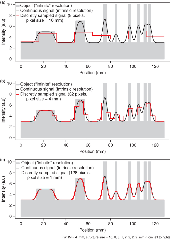
The black curve is the image of this object obtained at a given finite intrinsic spatial resolution of the imaging system. The implications of finite resolution with regards to quantitative measurements in the tomographic data are discussed in the next section. Here, we want to concentrate on the effects of final sampling, that is, of final pixel size. These effects can be appreciated when looking at the red curves in the figure. From Figure 2.1a–c, the number of pixels is increased consecutively by a factor of 4. When the pixel size decreases and falls sufficiently below the intrinsic spatial resolution (which is set to 4 mm in Fig. 2.1), the measured signal (the red curve) approximates the black curve with increasing accuracy. In Figure 2.1c the sampling is equal to the given estimate (four samples across the FWHM of the peaks). As explained earlier, this sampling density is more or less sufficient to restore the continuous signal (the black curves) from the discrete samples. At this sampling rate the discretized signal (the red curve) can itself serve as a reasonable approximation of the object (without the need to actually use the sampling theorem). Decreasing the pixel size (at the expense of increasing the total number of pixels) much further would not result in a better spatial resolution but only in an increase of image size and, thus, computer memory usage.
On the other hand (Fig. 2.1a and b), if the pixel size is larger than the intrinsic resolution of the imaging device, the effective resolution in the image is limited by this inadequate pixel size. This results in increasing loss of detail (different peaks no longer resolved) and discretization artifacts such as apparent shift of peak position and discontinuous jumps in image intensity. In our example, at the largest pixel size (Fig. 2.1a) the four separate peaks at the right hand side are no longer resolved.
In summary, one has to choose a pixel size that is adapted to the given resolution of the imaging device. As a rule of thumb, the pixel size should not exceed one half of the effective peak width (i.e., FWHM) in order to keep discretization errors tolerable, and reducing the pixel size by another factor of 2 (resulting in 4 pixels across the FWHM) is generally a good choice.
2.4 Consequences of Limited Spatial Resolution
A major figure of merit for any tomographic technique is the achieved spatial resolution. Table 2.1 gives some typical numbers for the major approaches discussed here.
Table 2.1 Typical Spatial Resolution of Different Tomographic Techniques
| Typical Spatial | |
| Technique | Resolution (mm) |
| Clinical CT | 1 |
| Clinical MRI | 1 |
| Clinical PET | 5 |
| Small animal CT | 0.03 |
| Small animal MRI | 0.06 |
| Small animal PET | 1.5 |
These values are valid for the primary image plane (which usually will be the transaxial plane). As has been indicated, modern tomographs are able to provide near-isotropic resolution in all three dimensions, that is, the resolution along the scanner axis is very nearly identical to that achieved in the transaxial plane.
Now, what exactly is meant by this kind of number, that is, what does it mean if spatial resolution is specified as being equal to 1 mm? Only the case of isotropic (direction independent) resolution will be discussed, but the adaption to the nonisotropic case should be straightforward.
Generally, spatial resolution is characterized by the Point Spread Function (PSF).
The PSF is the image of a point source (i.e., an infinitely small source; in practice this is a source whose linear dimensions are much smaller than the spatial resolution of the imaging device under consideration). The precise shape of the PSF depends on the imaging device, but usually a three-dimensional Gaussian
![]()
is an adequate description. (This might be seen as a consequence of the central limit theorem of mathematical statistics: each superposition of sufficiently many random processes with a probability density function dropping sufficiently rapid to zero for large deviations from the mean yields a normal distribution. In the current context, this corresponds to the superposition of the large number of factors contributing to the spatial resolution of the finally resulting tomographic image data.) The standard deviation σ of this Gaussian describes the spatial resolution. Instead of using σ, it is more common to specify the FWHM of the PSF (simply because this figure is directly accessible in measurements). The FWHM is the distance of the two points left and right of the center where the PSF has dropped to 50% of its center (maximum) value. For the Gaussian, the relation with the standard deviation σ is given by
![]()
that is, as a rule of thumb the FWHM is about twice the size of σ. The FWHM is not the strict limit for the minimal distance necessary to differentiate between two structures within the image. Rather, this figure is an approximate limit near which differentiation becomes increasingly difficult. This is illustrated in Figure 2.1. The two rightmost peaks have a distance equal to the FWHM of 4 mm and are barely discriminated in the measured signal. In the presence of image noise, differentiation of these two peaks would no longer be possible at all.
Loss of identifiability of adjacent peaks is only one aspect of finite spatial resolution. Another one is the mutual “cross talk” of neighboring structures. This phenomenon is usually referred to as the Partial Volume Effect (PVE) with regards to a loss of signal intensity from the Region of Interest (ROI) and called spillover when referring to a (undesired) gain of signal intensity from neighboring high intensity structures. The effect can be appreciated in Figure 2.1 in several respects by comparing the continuous signal with the true object. For one, all object boundaries exhibit an apparent smooth transit in signal intensity between target and background (loss of precise definition of the boundaries). Moreover, closely neighbored peaks acquire a slightly elevated signal intensity from the mutual cross talk of the signal intensities in comparison to a more distant peak of the same size (see the group of the four 2-mm peaks at the right hand side of the figure). At the same time, the target to background contrast is heavily reduced because of signal spillover into the background region between the peaks.
Another important aspect of limited spatial resolution is the limited recovery of the correct original signal intensity even for well isolated peaks. In order to assess the effect quantitatively, the Recovery Coefficient (RC) is used, which is defined as the ratio (after background subtraction) of the measured signal intensity maximum to the true intensity of the respective structure. As shown in Figure 2.1, the measured peaks only reach the original signal intensity if the size of the imaged structure is significantly larger than the spatial resolution limit as described by the FWHM.
Recovery limitation massively limits structure identification simply by decreasing the signal to background ratio and frequently leads to underestimates of signal intensity. For the smallest structure in Figure 2.1 (with a structure width of 1 mm, that is, 1/4 of the FWHM), the RC is less than 25% of the true signal intensity.
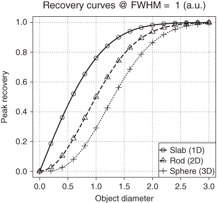
Limited recovery is an even more serious problem in the two- and three-dimensional case in comparison to the one-dimensional example of Figure 2.1. Figure 2.2 shows RC for homogeneous objects of three simple shapes for varying object size. By “slab” we designate an object whose spatial extent in two of its dimensions is much larger than the spatial resolution of the tomograph. The spatial extent in these dimensions can then be considered as “infinite” and does have no influence on the imaging process of cross sections through the slab. Therefore, the slab curve corresponds to the one-dimensional situation already shown in Figure 2.1. As a practical example, imaging of the myocardial wall corresponds approximately to this case, since the curvature of the myocardium is small compared to the spatial resolution (as well as compared to the wall thickness) and can therefore be neglected when estimating the recovery effects. Similarly, a (circular) “rod” is an object whose extent along one dimension can be considered as infinite and does not influence the cross-sectional imaging. This is thus the analog of simple two-dimensional imaging. As a practical example, consider imaging of the aorta or some other vessel. The third shape (sphere) approximates the imaging of localized structures whose extent in all three dimensions is comparable (as might be the case, e.g., for metastases of a tumor disease).
Figure 2.2 Recovery curves for three simple object shapes. The object diameter is specified in multiples of the FWHM of the PSF. If the object diameter drops below about two times the FWHM, recovery is rapidly decreasing, especially for rods and spheres.
For these simple object shapes (or any combination of them in order to describe more complex structures), simulation of the imaging process is rather straightforward (analytic convolution of the object with the PSF of the imaging device) and yields formulas that describe the spatial variation of the measured signal for any given spatial resolution (e.g., the continuous signal curve in Fig. 2.1 has been determined in this way).
The resulting formulas especially provide the intensity value at the center of the imaged structure. By dividing these values through the true intensity (i.e., by normalizing to unit intensity) one obtains the RC s as defined by the following expressions:
where
is the so-called error function and
![]()
For a more detailed discussion of recovery-related effects see (Kessler et al., 1984) (note that these authors use a different, and unusual, definition of the error function that might be a potential source of error when applying their formulas).
The RCs are not dependent on the absolute object size, but rather on the size of the object relative to the spatial resolution of the imaging device. Reducing at the same time object size and the width of the PSF by the same factor leaves the recovery unaltered. The curves in Figure 2.2 show the (peak) RCs as explained earlier, that is, the ratio of the measured peak intensity (in the center of the object) to the true intensity (which is assumed to be constant across the object). The recovery values approach a value of one only for object diameters of about three times the FWHM. For smaller objects, recovery decreases, most rapidly in the 3D case. The differences between the curves become very large for objects smaller than the FWHM. Already at a diameter of one-half of the FWHM, the peak recovery for a sphere is below 5% and about a factor of 10 smaller than for a slab of the same diameter. In the presence of finite image noise and background, such a small sphere will most probably not even be detectable, let alone assessable in any quantitative fashion.
These cumulative adverse consequences of limited spatial resolution and image noise are demonstrated in Figure 2.3, which uses the same sampling as in Figure 2.1c and superimposes noise on the measured signal.
Figure 2.3 Influence of image noise and finite spatial resolution (using the same configuration as in Fig. 2.1). For a given signal level, image noise most seriously affects structures near the resolution limit.
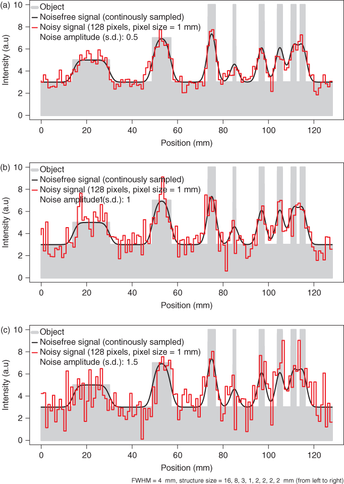
As can be seen by comparison with Figure 2.1c, objects near the resolution limit can no longer be correctly identified even at rather low noise levels. Both discrimination of adjacent peaks as well as identification of isolated small structures are compromised.
Up to now the consequences of limited spatial resolution with regard to measured signal intensity and detectability have been discussed.
Another point of interest is how accurately object boundaries can be localized. Since all sharp edges present in the image are smeared out by the finite resolution, one has to decide where on the slope the true boundary is located. For arbitrary shapes, this question cannot easily be answered since this would require a reversal of the imaging process (deconvolution), which can at best be carried out approximately. It is useful, nevertheless, to investigate the situation encountered with the simple object shapes discussed earlier.
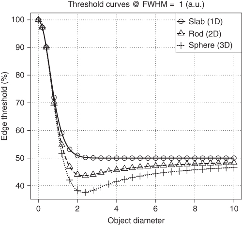
It turns out that for the one-dimensional case (“slab”), the object boundaries are usually located at a threshold of 50% of the peak intensity (after subtraction of potential background) except for very thin slabs near or below the resolution limit. Here the correct threshold becomes extremely size dependent and a reliable determination of object size is no longer possible.
In the two- and three-dimensional cases, it turns out that the threshold is generally size dependent and the threshold approaches the value of 50% only very slowly with increasing object size. This is illustrated in Figure 2.4 for the case of spheres.
Figure 2.4 Profile through the center of a sphere for three different sphere diameters. The solid horizontal line represents the threshold intersecting the profiles at the true object boundary. The threshold generally is size dependent and usually smaller than 50% except for very small sphere diameters.
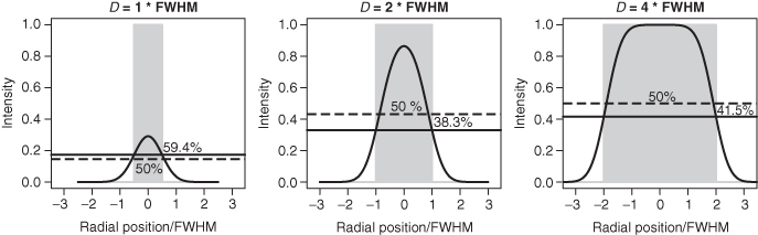
Figure 2.5 shows the resulting dependence of the “edge detecting” threshold for our three simple geometries as a function of object size. The object size dependence persists (for rods and spheres) well beyond the range where recovery limitations play a role. In contrast, the increase of the threshold at very small object sizes is simply a consequence of the rapidly decreasing RC in this range.
Figure 2.5 Object size dependence of the threshold intersecting the object boundary for three simple object shapes. The threshold is specified as a percentage of the measured (background corrected) signal maximum in the center of the object.
The situation described earlier imposes certain restrictions on the ability to delineate object boundaries in the image data correctly. If one resorts to interactive visual delineation of the object boundary in the image data, the uncertainties can be of the order of the FWHM, or even more, since the visual impression is very sensitive to details of the chosen color table and thresholding of the display. Depending on the relative size D/FWHM of the target structure and the question to be answered, this uncertainty might be irrelevant in one case and intolerable in the other. For example, for PET-based radiotherapy planning, unambiguous and accurate definition of boundaries is of paramount importance even for larger target structures.
It is therefore necessary to use algorithmic approaches that are able to account for effects such as those discussed above. Moreover, the presented results are valid in this form only under idealized circumstances (with respect to object shape, assumption of noise-free data, and Gaussian PSF and the assumption of an otherwise perfect imaging process). The lesson is that, for any given tomograph, it is necessary to investigate via phantom studies the exact behavior of the respective device under realistic circumstances and to use this information to optimize algorithmic approaches, which are able to perform the desired quantitatively correct object delineation.
2.5 Tomographic Data Evaluation: Tasks
2.5.1 Software Tools
Evaluation of tomographic data has two aspects: qualitative visual assessment of the images and extraction of quantitative data.
Any commercial tomograph will come together with a set of (possibly insufficient) evaluation tools. These will at least encompass 2D visualization facilities and functionality for defining two-dimensional ROIs. ROIs are finite size regions in the images for which the user desires to get quantitative measures (e.g., diameter, area, mean/minimum/maximum signal intensity). For ROI definition, the user can select between different options, including prescribed shapes (rectangles, circles, ellipses), irregular polygons, and threshold-based approaches.
Once the ROI is defined, the numerical data for the ROI are computed and usually saved to a text file for further processing.
If one looks at the visualization and data evaluation software accompanying the tomographs, usually some problems become apparent:
From these observations it follows that restricting oneself to the possibilities provided by the standard software tools coming with the tomograph is not reasonable. Instead, one should define the evaluation tasks and then look for the best tools available or, if this is an option, develop (part of) the necessary tools in-house.
Medical imaging is a highly technical field that requires dedicated tools. One consequence of this is that commercially provided tools are usually quite expensive. Nevertheless, prices for products providing similar functionality can vary extensively. It is always a good idea to check the availability of third-party products that sometimes are reasonable (or superior) alternatives to vendor-provided additional data evaluation workstations or “extension packages.”
Last, one should check out the tools that are provided as open Source or are otherwise are freely available in the public domain. As is true for other areas as well, there is a substantial amount of high quality software to be found here, which might suit the user's needs.
It would not make sense to give a comprehensive overview of the existing commercial and open source tools; such an overview would be outdated very rapidly, but two freely available and very valuable multipurpose tools should be mentioned: octave and R. Both can be used as interactive data exploration and visualization environments and include high level programming languages and numerical libraries, allowing the automation of complex data evaluation tasks without the need for low level programming in compiled languages (Eaton, 2011; R, 2011). A number of data processing tasks that are frequently relevant irrespective of which tomographic technique is used are discussed next.
2.5.2 Data Access
If one concludes that the available (or affordable) vendor-provided software tools are insufficient, the only remedy is to look for third-party software or implement the missing functionality in-house.
A necessary requirement is that the tomographic data are available in an accessible file format. A couple of years ago a multitude of proprietary file formats was still in use. Proprietary formats always pose the problem that interfacing the image data has to be solved for each vendor/modality separately.
The problem persists to a certain extent for the experimental devices used in small-animal imaging, but at least for the tomographic techniques that have found their way into clinical application one can safely expect that they provide the image data in a form compliant with the DICOM standard (DICOM Standards Committee, 2011).
Principally, adhering to a standard format is a good thing. With respect to DICOM, however, the standard is complex and allows for many vendor-specific entries (private tags) in the metadata part of the files. Interoperability between different vendors cannot always be taken for granted.
If one plans to process the images with third-party software or own tools, access to DICOM files is a must. Luckily, some noncommercial solutions exist, for instance, the DCMTK DICOM toolkit (OFFIS e.V., 2011), which provides a C library on top of which one's own applications can be built.
2.5.3 Image Processing
Once the access to the tomographic data is solved, the next requirement is to be able to perform standard image processing operations on the data. For slice-oriented (two-dimensional) processing of the tomographic data, one can resort to many different general purpose tools, but if the same tasks are to be performed on 3D image volumes, it is necessary to resort to programs specially designed for this. Generally, it is desirable to save the processed image data finally in the original source file format in order to make use of the available viewing software.
There are a number of recurring image processing tasks that one will encounter during evaluation of tomographic images.
2.5.3.1 Slice Averaging
This is the easiest way of achieving reduction of image noise and might especially be desirable if one deals with dynamic data where the statistical quality of each image volume is usually reduced because of shorter acquisition times. Averaging (or simply summing) slice ranges is nothing more than increasing the effective slice thickness of the tomographic images.
2.5.3.2 Image Smoothing
Image smoothing is one of the important tasks for which efficient tools should be available. The degree of smoothing defines the effective spatial resolution of the final images. For many tomographic methods it is not always wise to require that the full spatial resolution of the tomograph is used. Doing so necessarily increases the noise component in the images. If it turns out that the noise becomes so large that it masks relevant signals, using adequate smoothing is usually the only sensible strategy. From a formal point of view, smoothing is a special kind of filtering the data (namely low pass filtering). The mathematical framework for this is digital signal processing. There are a multitude of possible filter shapes possessing different properties. Depending on the precise characteristics of the input data, one can optimize the filter shape with respect to some desirable criteria. From a more pragmatic point of view, most filters that progressively suppress high frequency components (going sufficiently rapid to zero at high frequencies) perform well.
With respect to smoothing of 3D tomographic data, one should always use 3D filtering and avoid a slice-by-slice approach. It is thus possible to achieve a much better noise reduction for any given spatial resolution.
Smoothing can be described as operating in the frequency domain (the Fourier transform of the original data). This offers theoretical advantages and can be computationally more efficient for certain types of filters (e.g., bandpath filters). But usually it is more intuitive to describe smoothing as a weighted moving average operating directly on the discrete image data. The filter is defined by the filter kernel, which is the discretized equivalent of the intrinsic PSF of the imaging device; the filter kernel can be interpreted as the result one obtains when smoothing an image containing a single nonzero pixel. A two-dimensional example is given in Figure 2.6.
Figure 2.6 Example of image smoothing by using a two-dimensional moving average. (a) Original image matrix. (b) Smoothed image matrix obtained with the filter kernel ![]() .
.
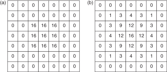
The smoothing process is achieved by centering the filter kernel in turn on each image pixel, computing the average of the covered pixels weighted with the corresponding values of the filter kernel and assigning the resulting value to the current center pixel. A reasonable smoothing filter should be symmetric around its center and include weights that decrease monotonically toward the filter edges.
Formally, one can view smoothing (or arbitrary filtering) as modifying the intrinsic PSF of the imaging device. In the case of smoothing, the PSF will become broader, that is, the spatial resolution decreases. In the 3D case, the filter kernel becomes a cube instead of a square, but the averaging process is the same. If the procedure described earlier is implemented literally, the computation time increases with the third power of the filter width. If filtering a given image volume with a kernel size of 3 × 3 × 3 would take 2 s, increasing the kernel size to 9 × 9 × 9 pixels would increase computation time by a factor of 27, that is, to about 1 min, making the approach unsuitable for large kernel sizes. One solution to the problem is to note that many filters, such as the one used in Figure 2.6, can be constructed from one-dimensional filters (in the above example from the single one-dimensional filter (1 2 1)) by multiplying the components of the one-dimensional filters that correspond to the coordinates in the multidimensional filters. For such separable filters it is much more efficient to perform three successive one-dimensional filterings along the three coordinates of the image volume. This yields exactly the same result as direct 3D filtering. The gain is especially dramatic for larger kernel sizes, since the computation time only increases linearly with the filter kernel size with this approach.
Reasonable 3D smoothing of the tomographic data can substantially improve the visual quality of the data; as discussed already, the data should be acquired with a pixel size that is smaller than the FWHM of the PSF of the tomograph. In this case, sizable intensity fluctuations between neighboring pixels will not correspond to actual signal variations in the imaged object, but will rather represent pure noise, that is, statistical fluctuations (Fig. 2.3). Filtering such data with a smoothing filter whose own effective FWHM is of the same order of magnitude than the intrinsic spatial resolution will deteriorate the final spatial resolution only to a limited extent but will reduce the noise amplitude massively.
Generally, the user should be aware that there always is a trade-off between maintaining maximal image resolution and minimizing noise. (This also holds true for the diametrical approach, namely trying to increase image resolution by deconvolving the PSF “out of” the measured data).
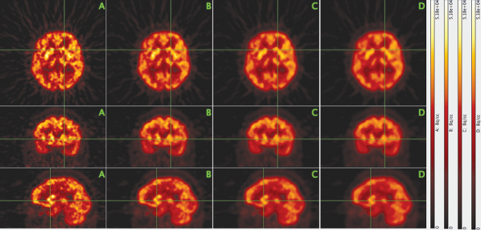
As an example, Figure 2.7 shows three orthogonal intersecting slices from a PET investigation of the human brain with the glucose analogue [18F]-2-fluoro-2-deoxy-D-glucose (FDG). The leftmost column shows the original data. The degree of three-dimensional smoothing increases through the columns from left to right. In the second column, the smoothing leads to a significant noise reduction while leaving the spatial resolution essentially unaltered. Only in the third and fourth columns a loss of resolution becomes obvious.
Figure 2.7 Effect of three-dimensional image smoothing on spatial resolution and noise level. Three orthogonal slices through the image volume from a PET investigation of the human brain with the glucose analogue FDG are shown (top row, transaxial; middle row, coronal; bottom row, sagittal). The leftmost column (A) shows the original image data that exhibit notable image noise. Columns B–D show the same slices after three-dimensional smoothing of the image volume with a cubic binomial filter kernel of width N = 3, 5, 7 pixels, respectively.
A cubic binomial filter kernel of width N = 3, 5, 7 was used in this example. The filter weights are defined by products of binomial coefficients3
![]()
where
![]()
For example, for N = 5, one gets w = (1, 4, 6, 4, 1). This type of filter is similar in effect to Gaussian shaped filters and offers the advantage that the kernel width alone defines the filter characteristic (for a Gaussian filter, the filter width should be matched to the standard deviation in order to yield sensible results).
In Figure 2.7, the spatial resolution corresponds to a FWHM of 3–4 pixels (in accord with our previous considerations concerning adequate sampling). Therefore, the 3 × 3 × 3 − point binomial smoothing used in column B affects the resolution only marginally, but reduces the image noise notably. Increasing the filter kernel size does cause a slight reduction of the image resolution but might still be found acceptable, depending on circumstances.
2.5.3.3 Coregistration and Resampling
Another frequently necessary operation is resampling of the image data, that is, modification of the voxel size. If one wants to maintain the originally covered image volume, this implies change of the 3D image matrix size as well. The need for this transformation regularly occurs if tomographic data from different modalities are to be compared side by side in a parallel display.
In order to evaluate spatially corresponding areas easily and reliably, it is necessary to ensure first that both data sets are displayed with respect to a common frame of reference. In principle, it would suffice to know the spatial transformation that connects the two native reference frames of both data sets (at least a coupled 3D rotation/translation is required). If this transformation is known, a display program could theoretically handle the parallel display (taking additionally into account the differing pixel sizes).
Practically, such an approach is not suitable for reasons of additional complications in data management as well as recurring computational overhead during visualization. Therefore, the usual procedure consists in transforming both data sets to a common voxel and image matrix size (resampling) and spatially transforming one of the image volumes to match the other (coregistration).
Coregistration is a well-investigated field, and there are several methods available. Automatic algorithms use variants of multidimensional optimization strategies to minimize some goodness of fit criterion, for example, the correlation coefficient between the intensities of corresponding pixels from both image volumes. The algorithms usually perform best for coregistration of image data from the same modality. Difficulties increase if there is a need for plastic transformations, as is generally the case for intersubject coregistration but possible also for intrasubject coregistration, for example, in the thorax.
Both operations (resampling and coregistration) imply interpolation within the image data. For reasons of increased numerical accuracy, it is therefore advantageous to combine both steps and to reduce the number of interpolations to one.
Interpolation becomes necessary because the image data are known only for the given discrete voxels. A reduction of the voxel size and/or spatial transformation of the imaged object then always requires to determine new values “in between” the given data. For practical matters, it usually suffices to use trilinear interpolation in the given data instead of using the full mathematical apparatus of the sampling theorem. A nearest neighbor approach, on the other hand, is usually inadequate.
2.5.4 Visualization
Tomographic data sets comprise large amounts of information. A single image volume can easily consist of several hundreds of slices. Therefore, efficient visualization tools are needed to analyze such data.
One useful technique is to navigate interactively through the image volumes with orthogonal viewers that allow the user to view simultaneously three orthogonal intersecting slices and to choose the slice positions interactively. Such viewers do exist as stand-alone applications or are integrated in dedicated data evaluation environments that offer additional functionality.
2.5.4.1 Maximum Intensity Projection (MIP)
The large number of tomographic images in a typical investigation makes it desirable to utilize efficient visualization techniques to augment (or sometimes even replace) the tedious slice-by-slice inspection of the primary tomographic data.
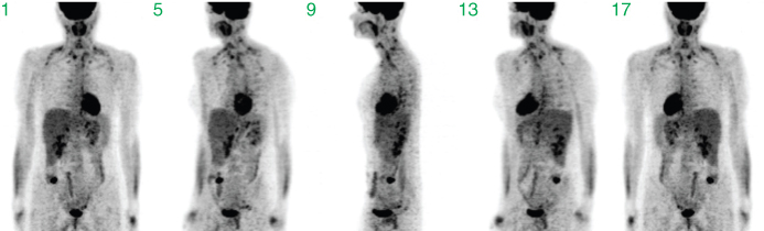
Initially, most tomographic techniques measure projection data. Each measured tomographic projection corresponds to a summation through the imaged volume along the given projection direction. The complete set of projections along sufficiently many directions is the basis for the tomographic image reconstruction, that is, the projection set already contains the complete information concerning the interior structure of the imaged object. Each single projection, on the other hand, contains only a small fraction of this information. The cumulative contribution from overlapping structures along the projection direction especially complicates identification (let alone localization) of smaller structures. This is illustrated in Figure 2.8, which shows projections along selected directions (in steps of 45°).
Figure 2.8 Sum projections along different directions. Shown are projections in angular steps of 45°, starting with a frontal view in projection 1. These data are part of the complete set of projection data from which the 3D tomographic volume is reconstructed.
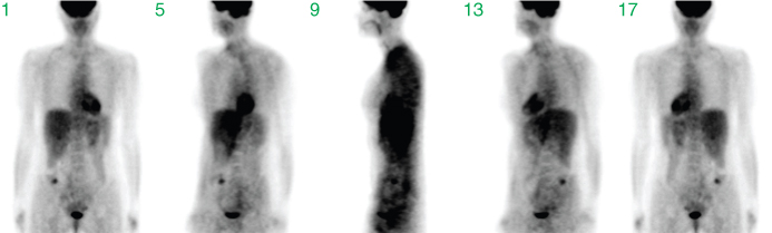
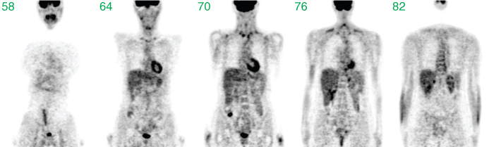
The visual quality is low. Only prominent structures such as the heart, the bladder, or the liver are identifiable. After image reconstruction (based on the complete set of all projections, not only the few shown in the figure), a detailed assessment of interior structures is possible, as demonstrated in Figure 2.9, where coronal slices from the resulting tomographic image volume are shown.
Figure 2.9 Selected coronal slices through the reconstructed tomographic image volume resulting from the complete set of projection data underlying Figure 2.8.
A comparison of the last two figures clearly demonstrates that the sum projections are usually not useful to get an alternative visualization of the tomographic data.
The idea of the Maximum Intensity Projection (MIP) consists in calculating projections through the tomographic image volume, but contrary to the initially measured sum projection data, one now looks for the maximum intensity pixel along each projection ray and uses its value in the projection image.
MIP is a very helpful method to get a quick overview of high signal intensity structures within an image volume. The approach works best for image data with high image contrast between target structures and the surrounding tissue.
In comparison to more sophisticated volume rendering algorithms, MIPs require only moderate computation time and might even be usable interactively in real-time if OpenGL support is available.
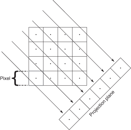
Usually the projection is performed within the transaxial image plane. Then, for each projection direction (from different angles around the edge of the transaxial slice), each transaxial slice contributes one row to the maximum projection image. Figure 2.10 illustrates this schematically.
Figure 2.10 Illustration of MIP. Along all projection rays through the tomographic image, the maxima that generate one row in the projection plane are determined. Repeating this procedure for the whole stack of transaxial tomographic images generates the maximum intensity image corresponding to this projection angle.
Each resulting maximum projection is completely overlap-free. The single pixel of maximum intensity (along the given projection direction) determines the intensity value in the projection image. However, each projection does not contain any depth information, since the maximum projection will look the same whether the maximum pixel in the tomographic data set was “at the front” or “at the back” of the data set. But if the maximum projection is repeated along multiple viewing directions, any high intensity structure in the image volume will be visible in many or all of the projections and the spatial location can be assessed. MIPs are especially suitable for generation of animations for which maximum projections are acquired at tightly spaced angles and then displayed as a cyclic movie, yielding the impression of a rotating semitransparent object, providing a view of the high intensity structures from different angles. However, this type of visualization is no substitute for a thorough assessment of the tomographic data themselves; MIPs will, for any given projection angle, display the maximum intensities along each projection ray, that is, hide everything else. If some structure is lying inside a high intensity “shell,” it will be completely invisible in a maximum projection. A central necrosis within a tumor, for instance, is not detectable at all in a MIP of a FDG-PET investigation, since the necrosis exhibits a much lower FDG uptake than the tumor rim, which “masks” the interior in the MIPs (in Fig. 2.11, this masking occurs for the cavity of the heart).
Figure 2.11 Example of volume rendering with maximum intensity projections (MIPs). Shown are projections in angular steps of 45°, starting with a frontal view in projection 1.
2.5.4.2 Volume Rendering and Segmentation
The maximum projection method is a simple and very useful visualization method in all situations where one is interested in well-defined (localized, high intensity) structures. The MIPs algorithm can be seen as the simplest example of a class of visualization techniques called volume rendering techniques.
Volume rendering is closely related to the problem of partitioning the image volume into different subvolumes (called segmentation) whose surfaces can then be displayed in different ways. One example of this is demonstrated in Figure 2.12.
Figure 2.12 Example of the combination of different 3D visualization techniques. Two tomographic data sets (CT and PET) of a human heart are shown. The CT data are displayed in gray via selected tomographic slices as well as maximum projections onto three orthogonal planes. In addition, the blood vessel geometry as derived by segmentation of the CT data is shown in red. The PET data are displayed semitransparently by volume rendering in green together with the segmented myocardial wall. The color used for the PET data display represents variations in myocardial blood flow that can be compared with the CT-derived information concerning blood vessel integrity. Courtesy of Prof. W. Burchert, Department of Radiology, Nuclear Medicine and Molecular Imaging, Heart and Diabetes Center, NRW, Germany.
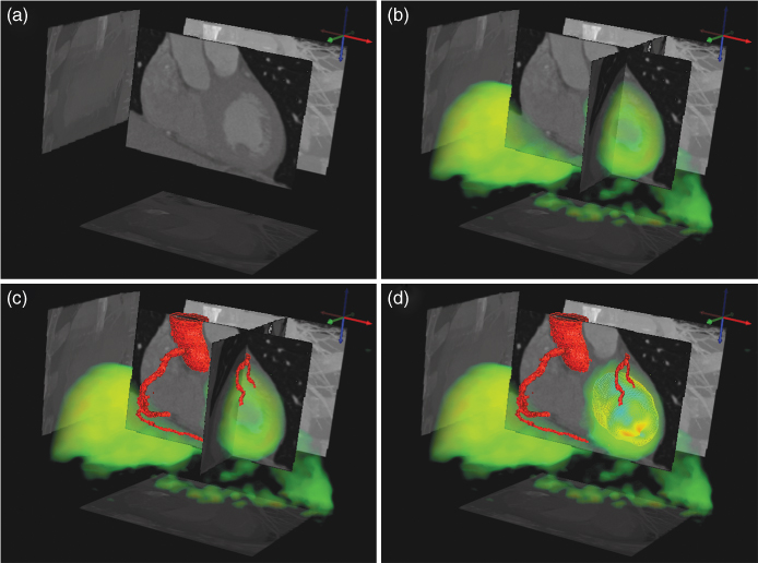
This example shows CT and PET data of a human heart and combines several techniques of visualizing the data: tomographic slices, maximum projections, semitransparent volume rendering, and segmentation. This example combines the detailed anatomical structure of the coronary arteries (derived from the CT data set) with the metabolic information present in the PET data.
2.5.5 Dynamic Tomographic Data
If one acquires a whole series of time “frames” (image volumes) in order to investigate dynamic processes, one ends up with a fourth data dimension (besides the three spatial coordinates), identifying a single voxel in a single time frame. Such measurements are sometimes called 4D data sets (as in “4D CT”), but we prefer calling them simply dynamic data.
A related possibility is the acquisition of gated data sets that use a stroboscopic method to visualize the cyclic motion of the heart and the lung: external triggers (ECG or a breathing trigger) are used to monitor and subdivide the motion cycle into several “gates,” which are mapped into separate image volumes. Each volume takes up a certain phase of the cyclic motion averaged over the duration of the data acquisition. One benefit of gating is the ability to correct for motion artifacts related to cyclic organ movement during the breathing cycle.
Dynamic measurements open up several possibilities not offered by static measurements since they allow the monitoring of in vivo physiological transport and metabolic processes. It is then possible to derive quantitative information for parameters such as blood flow, oxygen consumption, and blood volume for one or several ROIs or even each individual pixel within the tomographic image volume.
This ability to noninvasively quantify regional blood flow and metabolism is one of the strengths of the PET method. Apart from the possibility of using the biologically relevant molecules as tracers by labeling them with a suitable isotope, PET is superior to other tomographic methods because of the very good quantitative nature of the measurement process, which yields the regional tracer concentrations in absolute numbers, and its strict adherence to the tracer principle (introducing negligible amounts of the substance into the organism), which ensures that the measurement does not influence the investigated biological process.
Consequently, the kinetics of PET tracers can be treated as strictly linear, which allows the straightforward use of compartment modeling for the derivation of relevant parameters.
In principle, mathematical techniques similar to those used in PET can also be used to analyze contrast agent kinetics in CT or MRI. On closer inspection, however, the data evaluation is complicated by several factors. One of these factors concerns deviation from linearity because of the use of sizable amounts of contrast agent. This leads to deviations from linear kinetics (doubling the administered amount no longer doubles the response) as well as pharmacological effects that influence the outcome. For instance, one CT-based technique for the assessment of cerebral blood flow is based on administering stable xenon in sizable amounts that diffuse easily into brain tissue. The blood-flow-driven washout of xenon is then used to derive quantitative values for the local cerebral blood flow, in much the same mathematical way as when using PET with a freely diffusible tracer (such as 15O-labeled water). But since xenon is an anesthetic and has to be administered in sizable amounts, this leads to pharmacological effects (drowsiness). It cannot be taken for granted that cerebral blood flow is unaffected by this circumstance.
More recently, perfusion CT, which analyzes the single pass kinetics of common intravasal contrast agents using very high time resolution, has become a very active field. The potential of this technique is obvious, but there remain open questions with regard to systematic accuracy and validity of the mathematical techniques applied (Ng et al., 2006; Stewart et al., 2006; St Lawrence et al., 1998; van den Hoff, 2007a; van den Hoff, 2007b).
2.5.5.1 Parametric Imaging
If quantitation of dynamic data is performed on a per-pixel basis, the results define a new tomographic image volume where the pixel values no longer represent the primary signal (e.g., tracer concentration, Hounsfield units) but yield directly the relevant biological information. This can be evaluated visually or quantitatively via suitable ROIs.
Such parametric images are a valuable way of maximizing the information accessible to the user. Since the parameters displayed in the images have a direct biological interpretation (blood flow, glucose consumption, etc.), the visible image contrast is directly interpretable in terms of these parameters. Usually this is not the case when looking at the underlying dynamic data itself. Only under favorable circumstances is it possible to select time frames from the series around a certain time point in such a way that the image content is approximately proportional to the actual quantity of interest.
2.5.5.2 Compartment Modeling of Tomographic Data
Only a basic account of this technique is given, and the reader is otherwise referred to the literature, for example, Carson, 2003; Lassen and Perl, 1979; van den Hoff, 2005; Willemsen et al., 2002.
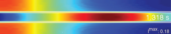
Compartment models describe the kinetics of tracers or contrast agents as bidirectional transport between several “well-stirred” pools, that is, spaces that do not exhibit any internal concentration gradients. This description seems a priori inadequate. For instance, the bolus passage of a tracer (or contrast agent) through the so-called Krogh cylinder is shown in Figure 2.13, as derived from a detailed mathematical convection/diffusion simulation. The “compartment assumption” of homogeneous distribution is fulfilled neither for the capillary nor for the surrounding tissue.
Figure 2.13 Numerical simulation of the capillary transit of a very short bolus of a permeable contrast agent or tracer through the Krogh cylinder. A longitudinal cross section through the capillary and surrounding tissue is shown. The capillary wall is indicated by the pair of white lines; the color indicates the concentration (blue, low; red, high) of the injected substance. The tracer is entering from the left at t = 0.Imax is the maximum concentration (specified as a fraction of the initial bolus amplitude at t = 0) in the system at the given time point t = 1.3 s.
Nevertheless, compartment models are frequently able to describe the measured data well and rarely lead to sizable bias in the derived parameters. Only at time scales shorter than the capillary transit time (requiring a corresponding time resolution of the experimental data), the compartment model description is no longer suitable.
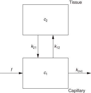
For dynamic tomographic data, however, compartment models are usually adequate. Figure 2.14 shows the first step of translating the situation in Figure 2.13 to a workable compartment model.
Figure 2.14 Linear chains of compartments describe the longitudinal concentration variations visible in Figure 2.13, where f specifies the perfusion, that is, the blood flow in units of (ml blood/min)/(ml tissue), c is tracer concentration, and k are rate constants (units min−1). Referring, as usual in compartment modeling, all concentrations to the common total volume of the system have consequences for the interpretation of the model parameters (e.g., the apparent asymmetry of k vs k and f vs k).
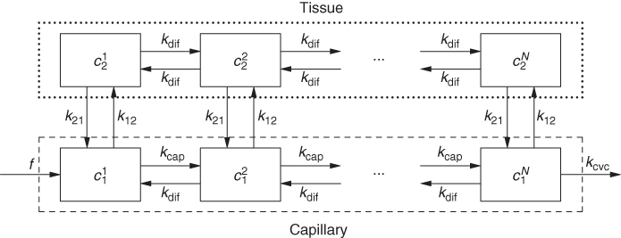
In this model, the longitudinal concentration gradients are accounted for by subdividing the capillary and surrounding tissue into sufficiently short sections for which all internal gradients are negligible. In mathematical terms, going from Figure 2.13 to Figure 2.14 is equivalent to replacing a partial differential equation with a system of ordinary differential equations that is much easier to solve.
Depending on the nature of the investigated system and/or the actual time resolution of the experimental data, this model configuration might be simplified further. In this example, at the usual time resolution of dynamic tomographic data, it is usually not possible to resolve details of the bolus passage. In Figure 2.15, all concentration gradients inside the capillary and the tissue are ignored (the behavior of the system can be described sufficiently using the average concentrations in these spaces, which is a weaker assumption, as it only assumes that potential concentration gradients are stationary). This configuration represents a two-compartment model, modeling the capillary space as one of the compartments. Such a description might be adequate when modeling the transit of a CT-contrast agent bolus imaged with high time resolution.
Figure 2.15 After the end of the capillary transit, the chain shown in Figure 2.14 can be collapsed into a single segment, which suffices to describe the “visible” tracer kinetics. For finite bolus duration (longer than the capillary transit time), this approach might also be adequate to describe the capillary transit itself.
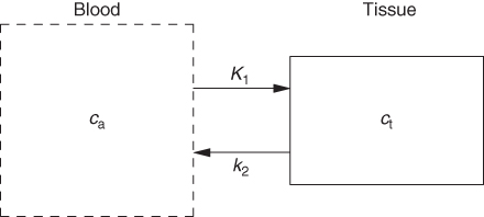
It is possible to simplify the description even further, as depicted in Figure 2.16. This configuration represents a one-compartment model, assuming that the capillary promptly follows every concentration change in the arterial input. This description is adequate for description of diffusible (reversibly transported) tracers in PET.
Figure 2.16 A further simplification, regularly applicable in PET (and generally for a time resolution not better than about 1 s), assumes that the time course of tracer concentration in the capillary blood space is identical to that in the arterial blood vessels.
The differences between the configurations in Figures 2.15 and 2.16 can be subtle, as demonstrated in Figure 2.17.
Figure 2.17 Simulated capillary passage of an idealized short bolus (red triangles) for a semipermeable contrast agent or tracer (time scale given in seconds). (a) The model from Figure 2.15 is used to generate a noisy artificial response curve (black circles) to which the model is fitted, yielding the decomposition in contributions from the capillary and from the tissue compartment. (b) The model from Figure 2.16 is used to fit the same artificial response curve. The capillary contribution is not modeled separately. Even in this idealized case, the data do not allow decision between the models.
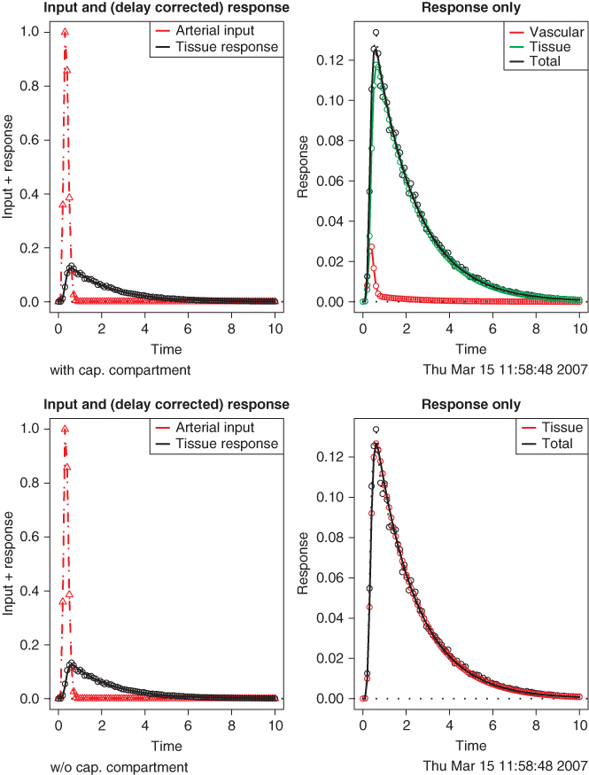
Both models fit the data well. Thus, selection of the correct model, which influences interpretation of the derived model parameters, must be done beforehand using available a priori information.
The above example is a special simple case. If the tracer kinetics is more complicated (e.g., if the tracer is trapped in the tissue or undergoes further metabolic steps), the compartment model has to account for this by adding further tissue compartments. In any case, the resulting model describes the measured data using standard optimization techniques to derive the model parameter values that yield the best fit of the model to the data. Performing this analysis on a per-pixel basis enables the generation of parametric images as explained in Section 2.5.5.1.
2.6 Summary
Evaluation of tomographic data combines techniques from digital signal processing, image processing, multidimensional data visualization, and numerical mathematical methods related to modeling and fitting the experimental data. It also includes the tomographic image reconstruction itself.
Depending on the tomographic technique and the special question investigated, emphasis might lie on qualitative evaluation and, thus, on image processing and visualization or on derivation of quantitative measures by developing adequate models and utilizing them for data description.
Generally, all aspects play an equally important role. Adequate integration of all steps in the data evaluation ensures that the wealth of detailed information present in tomographic data is used in an optimal way.
Notes
1 This description is not really suitable for all techniques. For example, in the case of magnetic resonance imaging the raw data are not projection data but are rather directly acquired in Fourier space. Moreover, in this case, directional information does not stem from the applied rf field itself but from its combination with a suitable gradient of the magnetic field utilized in the measurement. The basic strategy of using a penetrating radiation applies nevertheless.
2 We view sampling here as being contiguous across the data so that each pixel contains the average of the input signal over the pixel extension (histogramming). A slightly different, more common definition would be to represent the imaging process by equally spaced “point samples” from the continuous input signal. The difference between both definitions is small for densely sampled data but can be notable otherwise. For the tomographic techniques discussed here, the histogramming description is more adequate.
3 To simplify the formulas, we omit the necessary normalization to a value of one for the sum over all weights in the 3D filter kernel. Of course, this normalization should actually be included.
Carson RE. Tracer kinetic modeling in PET. In: Valk PE, Bailey DL, Townsend DW, Maisey MN, editors. Positron Emission Tomography. London: Springer; 2003. pp. 147–179, ISBN 1852334851.
DICOM Standards Committee. Digital Imaging and Communications in Medicine. 2011. Available at http://medical.nema.org.
Eaton JW. GNU Octave; 2011. Available at http://www.octave.org.
Gonzalez RC, Woods RE. Digital Image Processing (Prentice Hall International); 2007. pp. 976 ISBN 013168728X.
Kessler RM, Ellis JR Jr, Eden M. Analysis of emission tomographic scan data: limitations imposed by resolution and background. J Comput Assist Tomogr 1984;8(3):514–522.
Lassen N, Perl W. Tracer Kinetic Methods in Medical Physiology. New York: Raven Press; 1979, ISBN 0-89004-114-8.
Ng QS, Goh V, Fichte H, Klotz E, Fernie P, Saunders MI, Hoskin PJ, Padhani AR. Lung cancer perfusion at multi-detector row CT: reproducibility of whole tumor quantitative measurements. Radiology 2006;239(2):547–553.
Nyquist H. Certain topics in telegraph transmission theory. Trans AIEE 1928;47: 617–644.
OFFIS e.V. DCMTK - DICOM Toolkit. 2011. Available at http://www.dcmtk.org.
R Development Core Team. R: A Language and Environment for Statistical Computing. Vienna, Austria: R Foundation for Statistical Computing; 2011. ISBN 3-900051-07-0. Available at http://www.R-project.org.
Shannon CE. Communication in the presence of noise. Proc Inst Radio Eng 1949;37(1):10–21.
Stewart EE, Chen X, Hadway J, Lee TY. Correlation between hepatic tumor blood flow and glucose utilization in a rabbit liver tumor model. Radiology 2006;239(3):740–750.
St Lawrence KS, Lee TY. An adiabatic approximation to the tissue homogeneity model for water exchange in the brain: I. Theoretical derivation. J Cereb Blood Flow Metab 1998;18(12):1365–1377.
van den Hoff J. Principles of quantitative positron emission tomography. Amino Acids 2005;29(4):341–353.
van den Hoff J. Assessment of lung cancer perfusion using patlak analysis: what do we measure? Radiology 2007a;243(3):907–908.
van den Hoff J. Blood flow quantification with permeable contrast agents: a valid technique? Radiology 2007b;243(3):909–910.
Willemsen ATM, van den Hoff J, Quantitative PET. Fundamentals of data analysis. Curr Pharm Des 2002;8(16):1513–1526.