After our first few months of experimenting with robotics using the Mindstorms NXT kit, we began to wonder if there was a simple way to make our robot know where it was and where it was going—in other words, we wanted to create some kind of navigation system able to establish its position and direction. We started reading books and searching the Internet, and discovered that this is still one of most demanding tasks in robotics and that there really isn’t any single or simple solution.

In this chapter, we will introduce the concept of navigation, which can get very complex. We will start describing various positioning methods. Then we will provide some examples for these methods, showing solutions and tricks that suit the possibilities of the Mindstorms NXT system. In this discussion, we will introduce navigation on pads equipped with grids or gradients, use of laser beams to locate your robot in a room and explain how to equip your robot with sensors for the various measurements, and will provide the math to convert those measurements to determine your position.

There is no single method for determining the position and orientation of a robot, but you can combine several different techniques to get useful and reliable results. All these techniques can be classified into two general categories: absolute and relative positioning methods. This classification refers to whether the robot looks to the surrounding environment for tracking progress, or just to its own course of movement.

Absolute positioning refers to the robot using some external reference point to figure out its own position. These can be landmarks or obstacles in the environment, either natural landmarks or obstacles recognized through sensory inputs such as the touch, ultrasonic, magnetic compass sensors, or more often, artificial landmarks easily identified by your robot (such as colored tape on the floor). Another common approach includes using radio (or light) beacons as landmarks, like the systems used by planes and ships to find the route under any weather condition. Absolute positioning requires a lot of effort: you need a prepared environment, or some special equipment, or both.

Relative positioning, on the other hand, doesn’t require the robot to know anything about the environment. It deduces its position from its previous (known) position and the movements it made since the last known position. This usually is achieved through the use of encoders that precisely monitor the turns of the wheels, but there are also inertial systems that measure changes in speed and direction. This method also is called dead reckoning(short for deduced reckoning).

Relative positioning is quite simple to implement, and applies to our NXT robots, too. Unfortunately, it has an intrinsic, unavoidable problem that makes it impossible to use by itself: it accumulates errors. Even if you put all possible care into calibrating your system, there will always be some very small difference due to slippage, load, or tire deformation that will introduce errors into your measurements. These errors accumulate very quickly, thus relegating the utility of relative positioning to very short movements. Imagine you have to measure the length of a table using a very short ruler: you have to put it down several times, every time starting from the point where you ended the previous measurement. Every placement of the ruler introduces a small error, and the final result is usually very different from the real length of the table.

The solution employed by ships and planes, which use beacons like Loran or Global Positioning Systems (GPS) systems or reference earth’s magnetic field using Compass, is to combine methods from the two groups: to use dead reckoning to continuously monitor movements and, from time to time, some kind of absolute positioning to zero the accumulated error and restart computations from a known location. This is essentially what human beings do: when you walk down a street while talking to a friend, you don’t look around continuously to find reference points and evaluate your position; instead, you walk a few steps looking at your friend, then back to the street for an instant to get your bearings and make sure you haven’t veered off course, then you look back to your friend again.

You’re even able to safely move a few steps in a room with your eyes shut, because you can deduce your position from your last known one. But if you walk for more than a few steps without seeing or touching any familiar object, you will soon lose your orientation.

In the rest of the chapter, we will explore some methods for implementing absolute and relative positioning in NXT robots. It’s up to you to decide whether or not to use any one of them or a combination in your applications. Either way, you will discover that this undertaking is quite a challenge!

The most convenient way to place artificial landmarks is to put them flat on the floor, since they won’t obstruct the mobility of your robot and it can read them with a light sensor without any strong interference from ambient light. You can stick some self-adhesive tape directly on the floor of your room, or use a sheet of cardboard or other material over which you make your robot navigate.

Line following, which we have talked about in this book, is probably the simplest example of navigation based on using an artificial landmark. In the case of line following, your robot knows nothing about where it is, because its knowledge is based solely on whether it is to the right or left of the line. But lines are indeed an effective system to steer a robot from one place to another. Feel free to experiment with line following; for example, create some interruptions in a straight line and see if you are able to program your robot to find the line again after the break. It isn’t easy. When the line ends, a simple line follower would turn around and go back to the other side of the line. You have to make your software more sophisticated to detect the sudden change and, instead of applying a standard route correction, start a new searching algorithm that drives the robot toward a piece of line further on. Your robot will have to go forward for a specific distance (or time) corresponding to the approximate length of the break, then turn left and right a bit to find the line again and resume standard navigation.

When you’re done and satisfied with the result, you can make the task even more challenging: place a second line parallel to the first, with the same interruptions, and see if you can program the robot to turn 90 degrees, intercept the second line, and follow that one. If you succeed in the task, you’re ready to navigate a grid of short segments, either following along the lines or crossing over them like a bar code.

You can improve your robot navigation capabilities, and reduce the complexity in the software, using more elaborate markers. The NXT light sensor is not very good at distinguishing different colors, but is able to distinguish between differences in the intensity of the reflected light. You can play with black and gray tapes on a white pad, and use their color as a source of information for the robot. Remember that a reading at the border between black and white can return the same value of another on plain gray. Move and turn your robot a bit to decode the situation properly, or employ more than a single light sensor if you have them. Alternatively, you could use the color sensor (sold separately by LEGO) with your own color-coded markers.

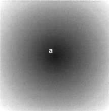
Instead of placing marks on the pad, you can also print on it with a special black and white gradient. For example, you can print a series of dots with an intensity proportional to their distance from a given point A. The closer to A, the darker the point; A is on plain black (see Figure 13.1). On such a pad, your robot will be able to return to A from any point, by simply following the route until it reads the minimum intensity.

Figure 13.1. A Gradient Pad with a Single Attractor

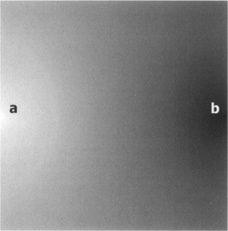
The same approach can be used with two points A and B, one being white and the other black. Searching for the whitest route, the robot arrives at A, whereas following the darkest it goes to B (see Figure 13.2).

Figure 13.2. A Gradient Pad with Two Attractors

RoboCup Junior uses a gradient pad for the soccer field. While searching for and chasing the ball, the robot could be anywhere on the field. When it gets the ball, it can refer to the pad below and with a light sensor, read the gray values and deduce how far it is from the goal. The same technique can then be used to detect which side is the opponent’s goal. Say the opponent’s goal is on the dark edge of the mat; the robot can spin around itself while measuring the gray values below, and deduce which side is the opponent’s goal.

Sub gradient_pad()
  padWidth = 50
  padHeight =50
  wPointX = padHeight / 2
  wPointY = 3
  bPointX = padHeight / 2
  bPointY = padWidth - 3


   For y = 1 To padWidth
      For x = 1 To padHeight
        whiteDist = Sqr((x - wPointX) * (x - wPointX) + (y - wPointY) * (y -wPointY))
        blackDist = Sqr((x - bPointX) * (x - bPointX) + (y - bPointY) * (y -bPointY))
        cValue = blackDist / (whiteDist + blackDist) * 255
        Cells(x, y).Interior.Color = RGB(cValue, cValue, cValue)
      Next x
    Next y
End Sub

Sub gradient_pad()
  padWidth = 50
  padHeight = 50


    For y = 1 To padWidth
       For x = 1 To padHeight
         cValue = y * (255 / padWidth)
         Cells(x, y).Interior.Color = RGBtcValue, cValue, cValue)
       Next x
     Next y
End Sub

The MINDSTORMS NXT kit comes with a pad that has gradient printed on the edge, for black and white as well as color use. This is a good place to start and experiment with.

There are other possibilities. People have suggested using bar codes on the floor: when the robot finds one, it aligns and reads it, decoding its position from the value. Others tried complex grids made out of stripes of different colors. Unfortunately, there isn’t a simple solution valid for all cases, and you will very likely be forced to use some dead reckoning after a landmark to improve the search.

Following the Beam

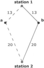
In the real world, most positioning systems rely on beacons of some kind, typically radio beacons. By using at least three beacons, you can determine your position on a two-dimensional plane, and with four or more beacons you can compute your position in a three-dimensional space. Generally speaking, there are two kinds of information a beacon can supply to a vehicle: its distance and its heading (direction of travel). Distances are computed using the amount of time that a radio pulse takes to go from the source to the receiver: the longer the delay, the larger the distance. This is the technique used in the Loran and the GPS systems. Figure 13.3 shows why two stations are not enough to determine position: because there are always two locations A and B that have the same distance from the two sources.

Figure 13.3. Ambiguous Positioning with Two Stations

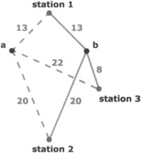
If you add a third station, the system can solve the ambiguity, provided that this third station does not lie along the line that connects the previous two stations (see Figure 13.4).

Figure 13.4. Positioning with Three Stations Using Distances

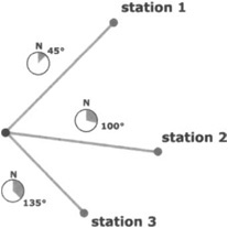
The stations of the VHF Omnidirectional Range system (VOR) cannot tell you the distance from the source of the beacon, but they do tell you their heading; that is, the direction of the route you should go to reach each station. Provided that you also know you’re heading north, two VOR stations are enough to locate your vehicle in most cases. Three of them are required to cover the case where the vehicle is positioned along the line that connects the stations, and as for the Loran and GPS systems, it’s essential that the third station itself does not lay along that line (see Figure 13.5).

Figure 13.5. Positioning with Three Stations Using Headings

Using three stations, you can do without a compass; that is, you don’t need to know you’re heading north. The method requires that you know only the angles between the stations as you see them from your position (see Figure 13.6).

Figure 13.6. Positioning with Three Stations Using Angles

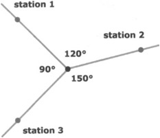
To understand how the method works, you can perform a simple experiment: take a sheet of paper and mark three points on it that correspond to the three stations. Now take a sheet of transparent material and put it over the previous sheet. Spot a point anywhere on it that represents your vehicle, and draw three lines from it to the stations, extending the lines over the stations themselves. Mark the lines with the name of the corresponding stations. Now, move the transparent sheet and try to intersect the lines again with the stations. An unlimited number of positions connect two of the three stations, but there’s only one location that connects all three of them.

The problem in this approach is, currently, there is no known device in the NXT world that would emit beacons, so first you have to look for an appropriate device. Unless you’re an electrical engineer and are able to design and build your own custom radio system, you better stick with something simple and easy to find. The source need not be necessarily based on radio waves—light is effective as well, and we already have such a detector (the light sensor) ready to interface to the NXT.

When you use light sources as small lighthouses, in theory you can make your robot find its way. But there are a few difficulties to overcome first:

• The light sensor isn’t directional—you must shield it somehow to narrow its angle.

• Ambient light introduces interference, so you must operate in an almost lightless room.

• For the robot to be able to tell the difference between the beacons, you must customize each one; for example, making them blink at different rates (as real lighthouses do).

Laser light is probably a better choice. It travels with minimum diffusion, so when it hits the light sensor, it is read at almost 100 percent. Laser sources are now very common and very cheap. You can find small battery-powered pen laser pointers for just a few dollars.

Warning

Laser light, even at low levels, is very damaging to eyes—never direct it toward people or animals.

If you have chosen laser as a source of light, you don’t need to worry about ambient light interference. But how exactly would you use laser? Maybe by making some rotating laser lighthouses? Too complex. Let’s see what happens if we revert the problem and put the laser source on the robot. Now you need just one laser, and can rotate it to hit the different stations. So, the next hurdle is to figure out how you know when you have hit one of those stations. If you place an NXT with a light sensor in every station, you can make it send back a message when it gets hit by the laser beam, and using different messages for every station, make your robot capable of distinguishing one from another.

The NXT light sensor is quite a small target to hit with a laser beam, and as a result, it was almost impossible to hit accurately. To stick with the concept but make things easier, we discovered you could build a sort of diffuser in front of it to have a wider detection area.

With this solution, you will still need several NXTs, at least three for the stations and one for your robot. Isn’t there a cheaper option? A different approach involves employing the simple plastic reflectors or reflective tapes used on cars, bikes, and as cat’s-eyes on the side of the road. You can find reflective tapes in your local art and craft stores. They have the property of reflecting any incoming light precisely back in the direction from which it came. Using those as passive “stations,” when your robot hits them with its laser beam they reflect it back to the robot, where you have placed a light sensor to detect it.

This really seems the perfect solution, but it actually still has its weak spots. First, you have lost the ability to distinguish one station from the other. You also have to rely on dead reckoning to estimate the heading of each station. We explained that dead reckoning is not very accurate and tends to accumulate errors, but it can indeed provide you with a good approximation of the expected heading of each station, enough to allow you to distinguish between them. After having received the actual readings, you will adjust the estimated heading to the measured one. The second flaw to the solution is that most of the returning beam tends to go straight back to the laser beam. You must be able to very closely align the light sensor to the laser source to intercept the return beam, and even with that precaution, detecting the returning beam is not very easy.

To add to these difficulties, there is some math involved in deducing the position of the robot from the beacons, and it’s the kind of math whose very name sends shivers down most students’ spines: trigonometry! This leads to another problem: the standard NXT firmware has no native support for trig functions, but in theory you could implement NXT-G blocks for such functions. If you want to proceed with using beacons, you really have to switch to RobotC or NBC, which both provide much more computational power.

If you’re not in the mood to face the complexity of trigonometry and alternative firmware, you can experiment with simpler projects that still involve laser pointers and reflectors. For example, you can make a robot capable of “going home.” Place the reflector at the home base of the robot; that is, the location where you want it to return. Program the robot to turn in place with the laser active, until the light beam intercepts the reflector and the robot receives the light back, then go straight in that direction, checking the laser target from time to time to adjust the heading.

Have you seen bats fluttering in evening twilight? Bats can get around just fine, doing their regular business in feeble light. Because, instead of light, they use sound to get around in the dark. In other words to “see” with their ears, they make sound in pulses. This sound reflects when it hits an object, and an echo bounces back to the bat. The time lapsed from making the sound and its echo tells the bat how far the object is. The ultrasonic sensor works on a similar principle.

You can use this technique to first detect your surroundings and recognize landmarks. Then you can use this information with a map to localize and establish your position.

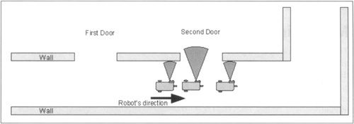
In this method information acquired from the sensors is compared to a map or model of the environment. If features from the sensor’s readings and the model map match, then the robot’s absolute location can be determined. In the previous example, these landmarks can be incorporated into your program to localize the robot. When the robot approaches a door, the ultrasonic sensor returns longer obstacle readings. These readings continue until the robot moves across the door. As shown in Figure 13.7, this information can help deduce that the robot has crossed the first door (or second door) and can identify its precise location.

Figure 13.7. The Ultrasonic Sensor Can Detect Surroundings and Recognize Landmarks

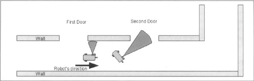
The inputs used in the preceding method included ultrasonic sensor readings, and a known map. Additional inputs can help improve accuracy. You could use distance from the wall, and orientation of the robot as additional inputs. The ultrasonic sensor would provide you the distance from the wall. These readings can be utilized with appropriate corrective action of wheel motors to maintain constant distance from the wall. However as shown in Figure 13.8, when unexpected drifts occur or objects appear in front of the ultrasonic sensor, the sensor will provide those readings too. You can either compare such readings with your previously known map information or ignore them. Better yet, you can use the additional input of a compass sensor to determine and maintain heading.

Figure 13.8. A Compass Sensor on the Robot Can Help Avoid Losing Orientation

A compass sensor would give you the magnetic heading your compass is pointing to. As your robot starts to maintain constant distance from the wall, note the heading from the compass sensor, and during subsequent movement maintain that heading by applying corrective action of wheel motors.

The technique of measuring the movement of the vehicle, called odometry, requires an encoder that translates the turn of the wheels into the corresponding traveled distance. To make things easier, the new NXT motors have a built-in encoder that is great for this purpose. To provide two degrees of freedom while moving, you typically will need two such motors, and as described in Chapter 3, you can also synchronize these two motors to get a straight-line motion.

The equations for computing the position from the decoded movements depends on the architecture of the robot. We will explain it here using the example of the differential drive, once again referring you to Appendix A for further resources on the math used.

Suppose that your robot has two wheels, each connected to a motor through gearing. Given D as the diameter of the wheel, R as the resolution of the built-in encoder in motors (the number of counts per turn), and G the gear ratio between the motor and the wheel, you can obtain the conversion factor F that translates each unit from the encoder into the corresponding traveled distance:

F = (D × π) /(G × R)

The numerator of the ratio, D × π, expresses the circumference of the wheel, which corresponds to the distance that the wheel covers at each turn. The denominator of the ratio, G×R, defines the increment in the count of the encoder (number of ticks) that corresponds to a turn of the wheel. F results in the unit distance covered for every tick.

Your robot uses the largest spoked wheels, which are 81.6mm in diameter. The built-in encoder of the motors has a resolution of 360 ticks per turn, and it is connected to the wheel with a 1:5 ratio (five turns of the sensor for one turn of the wheel). The resulting factor is:

F = 81.6 mm × 3.1416 / (5 × 360 ticks) - 0.14242 mm/tick

This means that every time the sensor counts one unit, the wheel has traveled 0.14242mm. In any given interval of time, the distance T_L covered by the left wheel will correspond to the increment in the encoder count l_L multiplied by the factor F:

T_L = l_L×F

and similarly, for the right wheel:

T_R = I_R × F

The centerpoint of the robot, the one that’s in the middle of the ideal line that connects the drive wheels, has covered the distance T_c:

T_c = (T_{R +} T_L)/2

To compute the change of orientation AO you need to know another parameter of your robot, the distance between the wheels B, or to be more precise, between the two points of the wheels that touch the ground:

ΔO = (T_R - T_L) / B

This formula returns AO in radians. You can convert radians to degrees using the relationship:

^ΔODegrees = ^ΔORadians ^{× 180/π}

You can now calculate the new relative heading of the robot, the new orientation O at time i based on previous orientation at time i – 1 and change of orientation AO. O is the direction in which your robot is pointed, and results in the same unit (radians or degrees) you choose for ΔO.

O_i = O_i-1 + ΔO

Similarly, the new Cartesian coordinates of the centerpoint come from the previous ones incremented by the traveled distance:

X_i = X_i-1 + T_c × COS O_i

y_i = y_i-1 + T_c× sin O_i

The two trigonometric functions convert the vectored representation of the traveled distance into its Cartesian components.

Oh,’ this villainous trigonometry again! Unfortunately, you can’t get rid of it when working with positioning. Thankfully, there are some special cases where you can avoid trig functions; for example, when you’re able to make your robot turn in place precisely 90 degrees, and truly go straight when you expect it to. In this situation, either X or Y remains constant, as well as the other increments (or decrements) of the traveled distance T_C.

The traveled distance can either be measured by the rotations of the motor that turns the wheels or the acceleration and velocity of the robot and the time it travels (the latter is called Inertial Navigation). You could use an acceleration sensor to measure acceleration of your robot.

The acceleration sensor measurements are influenced by the gravity of earth. So, if your robot is stationary on an inclined plane, you would still read a nonzero acceleration due to the gravitational influence. To correct that, you can use a gyroscopic sensor to know inclination of your robot.

If you are using the method of acceleration, in theory, the acceleration value A integrated over time T_Q to T_X will give you velocity V_x of your robot:

The velocity value V integrated over time TQ to T_x will give you the distance traveled.

There are third-party gyroscopic and acceleration sensors with varying sensitivity levels from HiTechnic and Mindsensors. These sensors can be used to measure acceleration of your robot. This seems easy if you know the formulae, but in practice a small error can result in unbounded growth in integrated measurements. To minimize errors, you need to take readings at rapid and constant intervals. With standard NXT firmware, it is almost impossible to achieve the required sampling rate.

We promised in the introduction that this was a difficult topic, and it was. Nevertheless, making a robot that has even a rough estimate of its position is a rewarding experience.

There are two categories of methods for estimating position, one based on absolute positioning and the other on relative positioning. The first category usually requires landmarks or beacons as external references. We described some possible approaches based on laser beams and introduced you to the difficulties that they entail. With the powerful I²C interface that NXT now offers, in future you can anticipate some advanced high-precision industrial positioning systems integrated with NXT. The Map Matching technique can make good use of Ultrasonic Sensor to read and verify map and determine position. It is possible to interface NXT robots with GPS systems, however outdoor GPS has granularity of 0.5 meters, which usually is inadequate for our robots.

Relative positioning is more readily applicable to NXT robots. We explained the math required to implement deduced reckoning in a differential drive robot, and suggested some alternative architectures that help in simplifying the involved calculations. We also explained how acceleration sensors could be utilized for measuring movements, and problems you may encounter. The real life navigation systems—like those used in cars, planes, and ships—usually rely on a combination of methods taken from both categories: dead reckoning isn’t very computation intensive and provides good precision in a short range of distances, whereas absolute references are used to zero the errors it accumulates.