Edited by Atif Khan
This chapter focuses on the following design implications of the Enhanced Interior Gateway Routing Protocol (EIGRP), Open Shortest Path First (OSPF) Protocols, and On-Demand Routing (ODR):
Network Topology
Addressing and Route Summarization
Route Selection
Convergence
Network Scalability
Security
EIGRP and OSPF are routing protocols for the Internet Protocol (IP). An introductory discussion outlines general routing protocol issues; subsequent discussions focus on design guidelines for the specific IP protocols.
The following discussion provides an overview of the key decisions you must make when selecting and deploying routing protocols. This discussion lays the foundation for subsequent discussions regarding specific routing protocols.
The physical topology of a network is described by the complete set of routers and the networks that connect them. Different routing protocols learn topology information in different ways. Some protocols require hierarchy and some do not. Networks require hierarchy in order to be scalable. Those protocols that do not require hierarchy should be designed with some level of hierarchy; otherwise, they are not scalable.
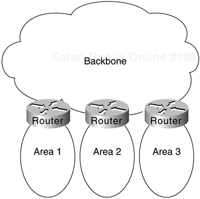
Some protocols require the creation of an explicit hierarchical topology through the establishment of a backbone and logical areas. The OSPF and Intermediate System–to–Intermediate System (IS-IS) protocols are examples of routing protocols that use a hierarchical structure. A generalhierarchical network scheme is illustrated in figure 3-1 The explicit topology in a hierarchical scheme takes precedence over the topology created through addressing.
With any routing protocol, the addressing topology should be assigned to reflect the hierarchy. There are two recommended ways to assign addresses in a hierarchical network. The simplest way is to give each area (including the backbone) a unique network address. An alternative is to assign address ranges to each area.
Areas are logical collections of contiguous networks and hosts. Areas also include all the routers having interfaces on any one of the included networks. Each area runs a separate copy of the basic routing algorithm. Therefore, each area has its own topological database.
Route-summarization procedures condense routing information. Without summarization, each router in a network must retain a route to every subnet in the network. With summarization, routers can reduce some sets of routes to a single advertisement, reducing both the load on the router and the perceived complexity of the network. The importance of route summarization increases with network size.
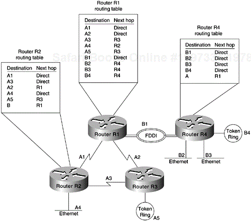
Figure 3-2 illustrates an example of route summarization. In this environment, Router R2 maintains one route for all destination networks beginning with B, and Router R4 maintains one route for all destination networks beginning with A. This is the essence of route summarization. Router R1 tracks all routes because it exists on the boundary between A and B.
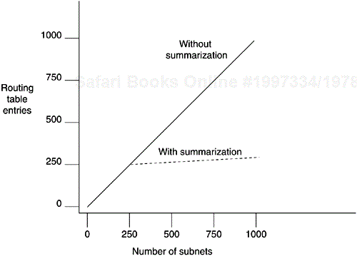
The reduction in route propagation and routing information overhead can be significant. Figure3-3 illustrates the potential savings. The vertical axis of Figure3-3 shows the number of routing table entries. The horizontal axis measures the number of subnets. Without summarization, each router in a network with 1,000 subnets must contain 1,000 routes. With summarization, the picture changes considerably. If you assume a Class B network with eight bits of subnet address space, each router needs to know all the routes for each subnet in its network number (250 routes, assuming that 1,000 subnets fall into four major networks of 250 routers each) plus one route for each of the other networks (three), for a total of 253 routes. This represents a nearly 75% reduction in the size of the routing table.
The preceding example shows the simplest type of route summarization: collapsing all the subnet routes into a single network route. Some routing protocols also support route summarization at any bit boundary (rather than just at major network number boundaries) in a network address. A routing protocol can summarize on a bit boundary only if it supports variable-length subnet masks (VLSMs).
Some routing protocols summarizeautomatically. Other routing protocols require manual configuration to support route summarization. Figure3-3 illustrates route summarization.
Route selection is trivial when only a single path to the destination exists. If any part of that path should fail, however, there is no way to recover. Therefore, most networks are designed with multiple paths so that there are alternatives in case a failure occurs.
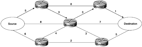
Routing protocols compare route metrics to select the best route from a group of possible routes. Route metrics are computed by assigning a characteristic or set of characteristics to each physical network. The metric for the route is an aggregation of the characteristics of each physical network in the route. Figure3-4 shows a typical meshed network with metrics assigned to each link, and the best route from source to destination identified.
Routing protocols use different techniques for assigning metrics to individual networks. Further, each routing protocol forms a metric aggregation in a different way. Most routing protocols can use multiple paths if the paths have an equal cost. Some routing protocols can even use multiple paths when paths have an unequal cost. In either case, load balancing can improve overall allocation of network bandwidth.
When multiple paths are used, there are several ways to distribute the packets. The two most common mechanisms are per-packet load balancing and per-destination load balancing. Per-packet load balancing distributes the packets across the possible routes in a manner proportional to the route metrics. With equal-cost routes, this is equivalent to a round-robin scheme. One packet or destination (depending on switching mode) is distributed to each possible path. Per-destination load balancing distributes packets across the possible routes based on destination. Each new destination is assigned the next available route. This technique tends to preserve packet order.
Note
Most TCP implementations can accommodate out-of-order packets. However, out-of-order packets may cause performance degradation.
When fast-switching is enabled on a router (default condition), route selection is done on a per-destination basis. When fast-switching is disabled, route selection is done on a per-packet basis. For line speeds of 56 kbps and faster, fast-switching is recommended.
When network topology changes, network traffic must reroute quickly. The phrase "convergence time" describes the time it takes a router to start using a new route after a topology changes. Routers must do three things after a topology changes:
Detect the change
Select a new route
Propagate the changed route information
Some changes are immediately detectable. For example, serial line failures that involve carrier loss are immediately detectable by a router. Other failures are harder to detect. If a serial line becomes unreliable but the carrier is not lost, for example, the unreliable link is not immediately detectable. In addition, some media (Ethernet, for example) do not provide physical indications such as carrier loss. When a router is reset, other routers do not detect this immediately. In general,failure detection depends on the media involved and the routing protocol used.
After a failure has been detected, the routing protocol must select a new route. The mechanisms used to do this are protocol-dependent. All routing protocols must propagate the changed route. The mechanisms used to do this are also protocol-dependent.
The capability toextend your network is determined, in part, by the scaling characteristics of the routing protocols used and the quality of the network design.
Network scalability is limited by two factors: operational issues and technical issues. Typically, operational issues are more significant than technical issues. Operational scaling concerns encourage the use of large areas or protocols that do not require hierarchical structures. When hierarchical protocols are required, technical scaling concerns promote the use of areas whose size is based on available resources, such as CPU, memory, and so on. Finding the right balance is the art of network design.
From a technical standpoint, routing protocols scale well if their resource use grows less than linearly with the growth of the network. Three critical resources are used by routing protocols: memory, central processing unit (CPU), and bandwidth.
Routing protocols usememory to store routing tables and topology information. Route summarization cuts memory consumption for all routing protocols. Keeping areas small reduces the memory consumption for hierarchical routing protocols.
CPU usage is protocol-dependent. Routing protocols use CPU cycles to calculate routes. Keeping routing information small by using summarization reduces CPU requirements by reducing the effect of a topology change and by decreasing the number of routes that must be recomputed after a topology change.
Bandwidth usage is also protocol-dependent. Three key issues determine the amount ofbandwidth a routing protocol consumes:
When routing information is sent—. Periodic updates are sent at regular intervals. Flash updates are sent only when a change occurs.
What routing information is sent—. Complete updates contain all routing information. Partial updates contain only changed information.
Where routing information is sent—. Flooded updates are sent to all routers. Bounded updates are sent only to routers affected by a change.
Note
These three issues also affect CPU usage.
Distance-vector protocols, such as Routing Information Protocol (RIP) andInterior Gateway Routing Protocol (IGRP), broadcast their complete routing table periodically, regardless of whether the routing table has changed. This periodic advertisement varies from every 30 seconds for RIP, to every 90 seconds for IGRP. When the network is stable, distance-vector protocols behave well, but, waste bandwidth because of the periodic sending of routing table updates, even when no change has occurred. When a failure occurs in the network, distance-vector protocols do not add excessive load to the network, but they take a long time to reconverge to an alternative path or to flush a bad path from the network.
Link-state routing protocols, such as Open Shortest Path First (OSPF), Intermediate System–to–Intermediate System (IS-IS), and NetWare Link Services Protocol (NLSP), were designed to address the limitations of distance-vector routing protocols (slow convergence and unnecessary bandwidth usage). Link-state protocols are more complex than distance-vector protocols, and use more CPU and memory. The additional overhead (in the form of memory utilization and CPU utilization) dictates the number of neighbors that a router can support and the number of routers that can be in an area. These numbers vary from network to network, and depend on variables such as CPU power, memory, number of routes, and link stability.
When the network is stable, link-state protocols minimize bandwidth usage by sending updates only when a change occurs. A hello mechanism ascertains reachability of neighbors. When a failure occurs in the network, link-state protocols flood link-state advertisements (LSAs) throughout an area. LSAs cause every router within the failed area to recalculate routes. The fact that LSAs need to be flooded throughout the area in failure mode and the fact that all routers recalculate routing tables dictate the number of routers that can be in an area.
EIGRP is an advanced distance-vector protocolthat has some of the properties of link-state protocols. EIGRP addresses the limitations of conventional distance-vector routing protocols (slow convergence and high bandwidth consumption in a steady-state network). When the network is stable, EIGRP sends updates only when a change in the network occurs. Like link-state protocols, EIGRP uses a hello mechanism to determine the reachability of neighbors. When a failure occurs in the network, EIGRP looks for new successors when there is no feasible successor present in the topology table by sending messages to its neighbors. The search for new successors can be aggressive in terms of the traffic it generates (updates, queries, and replies) to achieve convergence. This behavior constrains the number of possible neighbors.
InWANs, consideration of bandwidth is especially critical. Frame Relay, for example, which statistically multiplexes many logical data connections (virtual circuits) over a single physical link, allows the creation of networks that share bandwidth. Public Frame Relay networks use bandwidth sharing at all levels within the network. That is, bandwidth sharing may occur within the Frame Relay network of Corporation X, as well as between the networks of Corporation X and Corporation Y.
Two factors have a substantial effect on the design of public Frame Relay networks:
Users are charged for each permanent virtual circuit (PVC), which encourages network designers to minimize the number of PVCs.
Public carrier networks sometimes provide incentives to avoid the use of committed information rate (CIR) circuits. Although service providers try to ensure sufficient bandwidth, packets can be dropped.
Overall, WANs can lose packets due to a lack of bandwidth. For Frame Relay networks, this possibility is compounded because Frame Relay does not have a broadcast-replication facility; so for every broadcast packet sent out a Frame Relay interface, the router must replicate it for each PVC on the interface. This requirement limits the number of PVCs that a router can handle effectively.
In addition to bandwidth, network designers must consider the size of routing tables that need to be propagated. Clearly, the design considerations for an interface with 50 neighbors and 100 routes to propagate differ significantly from the considerations for an interface with 50 neighbors and 10,000 routes to propagate.
Controlling access to network resources is a primary concern. Some routing protocols provide techniques that can be used as part of a security strategy. With some routing protocols, you can insert a filter on the routes being advertised so that certain routes are not advertised in some parts of the network.
Some routing protocols can authenticate routers that run the same protocol. Authentication mechanisms are protocol-specific and generally weak. In spite of this, it is worthwhile to take advantage of the techniques that exist. Authentication can increase network stability by preventing unauthorized routers or hosts from participating in the routing protocol, whether those devices are attempting to participate accidentally or deliberately.
TheEnhanced Interior Gateway Routing Protocol (EIGRP) is a routing protocol developed by Cisco Systems, and introduced with Software Release 9.21 and Cisco Internetworking Operating System (Cisco IOS) Software Release 10.0. EIGRP combines the advantages of distance-vector protocols, such as IGRP, with the advantages of link-state protocols, such as Open Shortest Path First (OSPF). EIGRP uses the Diffusing Update Algorithm (DUAL) to achieve convergence quickly.
EIGRP includes support for IP, Novell NetWare, and AppleTalk. The discussion on EIGRP covers the following topics:
EIGRP Network Topology
EIGRP Addressing
EIGRP Route Summarization
EIGRP Route Selection
EIGRP Convergence
EIGRP Network Scalability
EIGRP Security
Note
Although this section is applicable to IP, IPX, and AppleTalk EIGRP, IP issues are highlighted here. For case studies on how to integrate EIGRP into IP, IPX, and AppleTalk networks, including detailed configuration examples and protocol-specific issues, see Chapter 17, "Configuring EIGRP for Novell and AppleTalk Networks."
EIGRP can use a nonhierarchical (or flat) topology. To design a scalable network, it is important to have hierarchy. EIGRP automatically summarizes subnet routes of directly connected networks at a network number boundary. For more information, see the section titled "EIGRP Route Summarization," later in this chapter.
The first step in designing an EIGRP network is to decide how to address the network. In many cases, a company is assigned a single NIC address (such as a Class B network address) to be allocated in a corporate network. Bit-wise subnetting andvariable-length subnetwork masks (VLSMs) can be used in combination to save address space. EIGRP for IP supports the use of VLSMs.
Consider a hypothetical network in which a Class B address is divided into subnetworks, and contiguous groups of these subnetworks are summarized by Enhanced IGRP. The Class B network 156.77.0.0 might be subdivided as illustrated in Figure3-5
In Figure3-5, the letters x, y, and z represent bits of the last two octets of the Class B network, as follows:
The four x bits represent the route summarization boundary.
The five y bits represent up to 32 subnets per summary route.
The seven z bits allow for 126 (128 – 2) hosts per subnet.
Appendix A, "Subnetting an IP Address Space," provides a complete example illustrating assignment for the Class B address 150.100.0.0.
With Enhanced IGRP, subnet routes of directly connected networks are automatically summarized at network number boundaries. In addition, a network administrator can configure route summarization at any interface with any bit boundary, allowing ranges of networks to be summarized arbitrarily.
Routing protocols compare route metrics to selectthe best route from a group of possible routes. The following factors are important to understand when designing an EIGRP network. EIGRP uses the same vector of metrics as IGRP. Separate metric values are assigned for bandwidth, delay, reliability, and load. By default, EIGRP computes the metric for a route by using the minimum bandwidth of each hop in the path and adding a media-specific delay for each hop. The metrics used by EIGRP are as follows:
Bandwidth—. Bandwidth is deduced from the interface type. Bandwidth can be modified with the bandwidth command.
Delay—. Each media type has a propagation delay associated with it. Delay can be modified with the delay command.
Reliability—. Reliability is dynamically computed as a rolling weighted average over five seconds.
Load—. Load is dynamically computed as a rolling weighted average over five seconds.
When EIGRP summarizes a group of routes, it uses the metric of the best route in the summary as the metric for the summary.
EIGRP implements a convergence algorithm known as DUAL (Diffusing Update Algorithm). DUAL uses two techniques that allow EIGRP to converge very quickly. First, each EIGRP router builds an EIGRP topology table by receiving its neighbors'routing tables. This allows the router to use a new route to a destination instantly if another feasible route is known. If no feasible route is known based on the routing information previously learned from its neighbors, a router running EIGRP becomes active for that destination and sends a query to each of its neighbors, asking for an alternative route to the destination. These queries propagate until an alternative route is found. Routers that are not affected by a topology change remain passive, and do not need to be involved in the query and response.
A router using EIGRP receives full routing tables from its neighbors when it first communicates with the neighbors. Thereafter, only changes to the routing tables are sent, and only to routers affected by the change. A successor is a neighboring router currently being used for packet forwarding, provides the least cost route to the destination, and is not part of a routing loop. When a route to a destination is lost through the successor, the feasible successor, if present for that route, becomes the successor. Feasible successors provide the next least cost path without introducing routing loops.
The routing table keeps a list of the computed costs of reaching networks. The topology table keeps a list of routes advertised by neighbors. For each network, the router keeps the real cost of getting to that network and also keeps the advertised cost from its neighbor. In the event of a failure, convergence is instant if a feasible successor can be found. A neighbor is a feasible successor if it meets the feasibility condition set by DUAL. DUAL finds feasible successors by performing the following computations:
Determines membership of V1. V1 is the set of all neighbors whose advertised distance to network x is less than FD. (FD is the feasible distance and is defined as the best metric during an active-to-passive transition.)
Calculates Dmin. Dmin is the minimum computed cost to network x.
Determines membership of V2. V2 is the set of neighbors in V1 whose computed cost to network x equals Dmin.
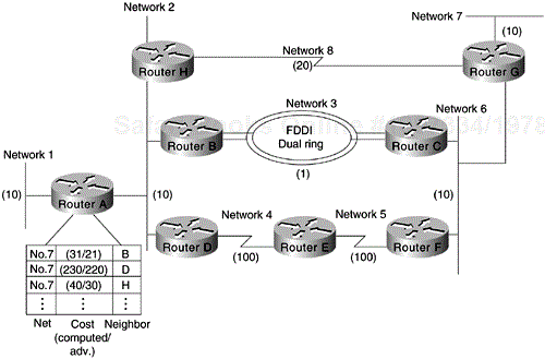
The feasibility condition is met when V2 has one or more members. Figure3-6 illustrates the concept of feasible successors. Consider Router A's topology table entries for Network 7. Router B is the successor with a computed cost of 31 to reach Network 7, compared to the computed costs of Router D (230) and Router H (40).
If Router B becomes unavailable, Router A will go through the following three-step process to find a feasible successor for Network 7:
Determining which neighbors have an advertised distance to Network 7 that is less than Router A's feasible distance (FD) to Network 7. The FD is 31, and Router H meets this condition. Therefore, Router H is a member of V1.
Calculating the minimum computed cost to Network 7. Router H provides a cost of 40, and Router D provides a cost of 230. Dmin is, therefore, 40.
Determining the set of neighbors in V1 whose computed cost to Network 7 equals Dmin (40). Router H meets this condition.
The feasible successor is Router H, which provides a least cost route of 40 from Router A to Network 7. If Router H now also becomes unavailable, Router A performs the following computations:
Determineswhich neighbors have an advertised distance to Network 7 that is less than the FD for Network 7. Because both Router B and H have become unavailable, only Router D remains. The advertised cost of Router D to Network 7 is 220, however, which is greater than Router A's FD (31) to Network 7. Router D, therefore, cannot be a member of V1. The FD remains at 31—the FD can only change during an active-to-passive transition, and this did not occur. There was no transition to active state for Network 7; this is known as a local computation.
Because there are no members of V1, there can be no feasible successors. Router A, therefore, transitions from passive to active state for Network 7 and queries its neighbors about Network 7. There was a transition to active; this is known as a diffusing computation.
Note
For more details on EIGRP convergence, see Appendix H, "References and Recommended Reading," for a list of reference papers and materials.
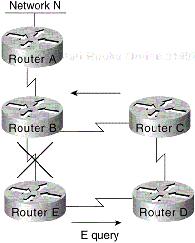
The following example and graphics further illustrate how EIGRP supports virtually instantaneous convergence in a changing network environment. In Figure3-7, all routers can access one another and Network N. The computed cost to reach other routers and Network N is shown. For example, the cost from Router E to Router B is 10. The cost from Router E to Network N is 25 (cumulative of 10 + 10 + 5 = 25).
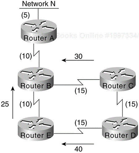
In Figure3-8, theconnection between Router B and Router E fails. Router E sends a multicast query to all of its neighbors and puts Network N into an active state.
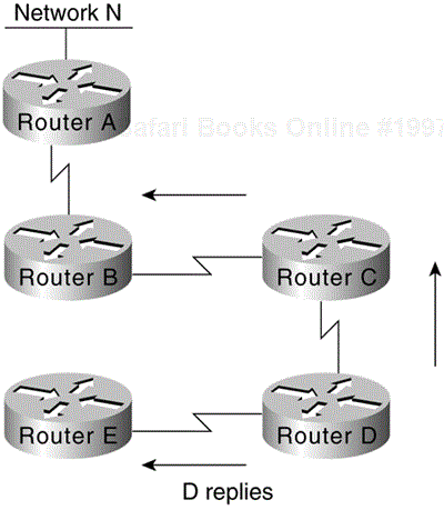
Next, as illustrated in Figure3-9, Router D determines that it has a feasible successor. It changes its successor from Router E to Router C and sends a reply to Router E.
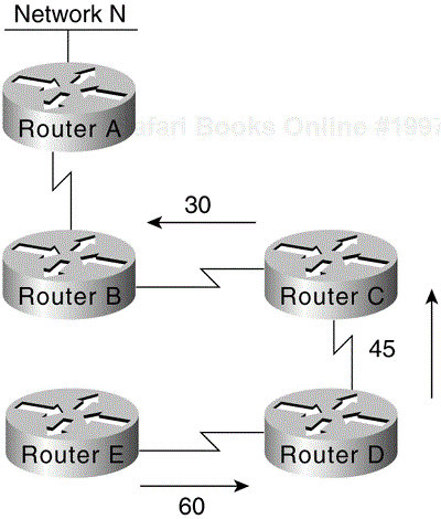
In Figure3-10, Router E has received replies from all neighbors and therefore brings Network N out of active state. Router E puts Network N into its routing table at a distance of 60.
Network scalability is limited by two factors: operational issues and technical issues. Operationally, EIGRP provides easy configuration. Technically, EIGRP uses resources at less than a linear rate with the growth of a network, if properly designed. Hierarchy, both physical and logical, is the key to designing a scalable EIGRP network.
A router running EIGRP stores routes advertised by neighbors so that it can adapt quickly to alternative routes. The more neighbors a router has, the more memory a router uses. EIGRP automatic route aggregation bounds the routing table growth naturally. Additional bounding is possible with manual route aggregation.
EIGRP uses the DUAL algorithm to provide fast convergence. DUAL recomputes only routes affected by a topology change. DUAL is not computationally complex, but utilization of the CPU depends on the stability of the network, query boundaries, and reliability of the links.
EIGRP uses partial updates. Partial updates are generated only when a change occurs; only the changed information is sent, and this changed information is sent only to the routers affected. Because of this, EIGRP is efficient in its usage of bandwidth. Some additional bandwidth is used by EIGRP's Hello protocol to maintain adjacencies between neighboring routers.
To create a scalable EIGRP network, you should implement route summarization. To create an environment capable of supporting route summarization, you must implement an effective hierarchical addressing scheme. The addressing structure that you implement can have a profound impact on the performance and scalability of your EIGRP network.
OSPF is an IGP developed for use in IP-based networks. As an IGP, OSPF distributes routing information between routers belonging to a single autonomous system (AS). An AS is a group of routers exchanging routing information via a common routing protocol. The OSPF protocol is based on shortest-path-first (SPF), or link-state, technology.
The OSPF protocol was developed by the OSPF working group of the Internet Engineering Task Force (IETF). It was designed expressly for the IP environment, including explicit support for IP subnetting and the tagging of externally derived routing information. OSPF Version 2 is documented in Request for Comments (RFC) 1247.
Whether you are building an OSPF network from the ground up or converting your network to OSPF, the following design guidelines provide a foundation from which you can construct a reliable, scalable OSPF-based environment.
Two design activities are critically important to a successful OSPF implementation:
Definition of area boundaries
Address assignment
Ensuring that these activities are properly planned and executed will make all the difference in your OSPF implementation. Each is addressed in more detail in the discussions that follow. These discussions are divided into nine sections:
OSPF Network Topology
OSPF Addressing and Route Summarization
OSPF Route Selection
OSPF Convergence
OSPF Network Scalability
OSPF Security
OSPF NSSA (Not-So-Stubby Area) Capabilities
OSPF On-Demand Circuit Protocol Issues
OSPF Over Nonbroadcast Networks
Note
For a detailed case study on how to set up and configure OSPF redistribution, see Chapter 16, "EIGRP and OSPF Redistribution."
OSPF works best in a hierarchical routing environment. The first and most important decision when designing an OSPF network is to determine which routers and links are to be included in the backbone, and which are to be included in each area. You should consider several important guidelines when designing an OSPF topology:
The number of routers in an area—. OSPF uses a CPU-intensive algorithm. The number of calculations that must be performed given n link-state packets is proportional to n log n. As a result, the larger and more unstable the area, the greater the likelihood for performance problems associated with routing-protocol recalculation. The size of an area depends on the router CPU, memory, and number of links in an area.
The number of neighbors for any one router—. OSPF floods all link-state changes to all routers in an area. Routers with many neighbors have the most work to do when link-state changes occur. Number of neighbors per router depends on router CPU, number of links in an area, CPU of the neighboring routers, and bandwidth of link to neighbors.
The number of areas supported by any one router—. A router must run the link-state algorithm for each link-state change that occurs for every area in which the router resides. Every Area Border Router is in at least two areas (the backbone and one area).
Designated router selection—. In general, the designated router and backup designated router on a local-area network (LAN) are adjacent to all neighbors. They have the responsibility of generating flooding LSAs of adjacent routes, as well as generating network link states on behalf of the network. It is a good idea to select routers that are not already heavily loaded with CPU-intensive activities to be the designated router and backup designated router.
The discussions that follow address topology issues specifically related to the backbone and the areas.
Stability and redundancy are the most important criteria for the backbone. Stability is increased by keeping the size of the backbone reasonable. The size of the backbone must be reasonable because each router in the backbone needs to recompute its routes after every link-state change. Keeping the backbone small reduces the likelihood of a change and reduces the amount of CPU cycles required to recompute routes. Redundancy is important in the backbone to prevent partition when a link fails. Good backbones are designed so that no single link failure can cause a partition.
OSPF backbones must be contiguous. OSPF includes the use of virtual links. A virtual link creates a path between two Area Border Routers (an Area Border Router is a router that connects an area to the backbone) that are not directly connected. A virtual link can be used to heal a partitioned backbone. It is not a good idea, however, to design an OSPF network to require the use of virtual links. The stability of a virtual link is determined by the stability of the underlying area. This dependency can make troubleshooting more difficult. In addition, virtual links cannot run across stub areas. See the section titled "Backbone-to-Area Route Advertisement," later in this chapter for a detailed discussion of stub areas.
Avoid placing hosts (such as workstations, fileservers, or other shared resources) in the backbone area. Keeping hosts out of the backbone area simplifies network expansion and creates a more stable environment.
Individual areas should be contiguous. An area can be partitioned, but it is not recommended. In this context, a contiguous area is one in which a continuous path can be traced from any router in an area to any other router in the same area. This does not mean that all routers must share common network media. The two most critical aspects of area design follow:
Determining how the area is addressed
Determining how the area is connected to the backbone
Areas should have a contiguous set of network or subnet addresses. Without a contiguous address space, it is not possible to implement route summarization. The routers that connect an area to the backbone are called Area Border Routers. Areas can have a single Area Border Router or they can have multiple Area Border Routers. In general, it is desirable to have more than one Area Border Router per area to minimize the chance of the area becoming disconnected from the backbone.
When creating large-scale OSPF networks, the definition of areas and assignment of resources within areas must be done with a pragmatic view of your network. The following are general rules that help ensure that your network remains flexible and provides the kind of performance needed to deliver reliable resource access:
Consider physical proximity when defining areas—. If a particular location is densely connected, create an area specifically for nodes at that location.
Reduce the maximum size of areas if links are unstable—. If your network includes unstable links, consider implementing smaller areas to reduce the effects of route flapping. Whenever a route is lost or comes online, each affected area must converge on a new topology. The Dykstra algorithm will run on all the affected routers. By segmenting your network into smaller areas, you can isolate unstable links and deliver more reliable overall service.
Address assignment and route summarization are inextricably linked when designing OSPF networks. To create a scalable OSPF network, you should implement route summarization. To create an environment capable of supporting route summarization, you must implement an effective hierarchical addressing scheme. The addressing structure that you implement can have a profound impact on the performance and scalability of your OSPF network. The following sections discuss OSPF route summarization and three addressing options:
Separate network numbers for each area
Network Information Center (NIC)–authorized address areas created using bit-wise subnetting and VLSM
Private addressing, with a demilitarized zone (DMZ) buffer to the official Internet world
Note
You should keep your addressing scheme as simple as possible, but be wary of oversimplifying your address-assignment scheme. Although simplicity in addressing saves time later when operating and troubleshooting your network, taking shortcuts can have certain severe consequences. In building a scalable addressing environment, use a structured approach. If necessary, use bit-wise subnetting—but make sure that route summarization can be accomplished at the Area Border Routers.
Route summarization is extremely desirable for a reliable and scalable OSPF network. The effectiveness of route summarization, and your OSPF implementation in general, hinge on the addressing scheme that you adopt. Summarization in an OSPF network occurs between each area and the backbone area. Summarization must be configured manually in OSPF. When planning your OSPF network, consider the following issues:
Be sure that your network addressing scheme is configured so that the range of subnets assigned within an area is contiguous.
Create an address space that will permit you to split areas easily as your network grows. If possible, assign subnets according to simple octet boundaries. If you cannot assign addresses in an easy-to-remember and easy-to-divide manner, be sure to have a thoroughly defined addressing structure. If you know how your entire address space is assigned (or will be assigned), you can plan more effectively for changes.
Plan ahead for the addition of new routers to your OSPF environment. Be sure that new routers are inserted appropriately as area, backbone, or border routers. Because the addition of new routers creates a new topology, inserting new routers can cause unexpected routing changes (and possibly performance changes) when your OSPF topology is recomputed.
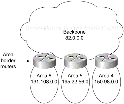
One of the simplest ways to allocate addresses in OSPF is to assign a separate network number for each area. With this scheme, you create a backbone and multiple areas, and assign a separate IP network number to each area. Figure3-11 illustrates this kind of area allocation.
The following are the basic steps for creating such a network:
In the network illustrated in Figure3-11, each area has its own unique address. These can be Class A (the backbone in Figure3-11), Class B (Areas 4 and 6), or Class C (Area 5). The following are some benefits of assigning separate address structures to each area:
Address assignment is relatively easy to remember.
Configuration of routers is relatively easy and mistakes are less likely.
Network operations are streamlined because each area has a simple, unique network number.
In the example illustrated in Figure3-11, the route-summarization configuration at the Area Border Routers is greatly simplified. Routes from Area 4 injecting into the backbone can be summarized as follows: All routes starting with 150.98 are found in Area 4.
The main drawback of this approach to address assignment is that it wastes address space. If you decide to adopt this approach, be sure that Area Border Routers are configured to do route summarization. Summarization must be explicitly set.
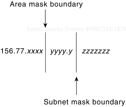
Bit-wise subnetting and variable-length subnetwork masks (VLSMs) can be used in combination to save address space. Consider a hypothetical network in which a Class B address is subdivided using an area mask and distributed among 16 areas. The Class B network, 156.77.0.0, might be subdivided as illustrated in Figure3-12.

In Figure3-12, the letters x, y, and z represent bits of the last two octets of the Class B network, as follows:
The four x bits are used to identify 16 areas.
The five y bits represent up to 32 subnets per area.
The seven z bits allow for 126 (128 – 2) hosts per subnet.
Appendix A, "Subnetting an IP Address Space," provides a complete example illustrating assignment for the Class B address 150.100.0.0. It illustrates both the concept of area masks and the breakdown of large subnets into smaller ones using VLSMs.
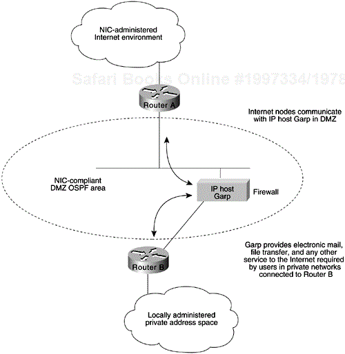
Private addressing is another option often cited as simpler than developing an area scheme using bit-wise subnetting. Although private address schemes provide an excellent level of flexibility and do not limit the growth of your OSPF network, they have certain disadvantages. Developing a large-scale network of privately addressed IP nodes limits total access to the Internet, for instance, and mandates the implementation of what is referred to as a demilitarized zone (DMZ). If you need to connect to the Internet, Figure3-13 illustrates the way in which a DMZ provides a buffer of valid NIC nodes between a privately addressed network and the Internet.
Note
For a case study on network security, including information on how to set up firewall routers and communication servers, see Chapter 22, "Increasing Security in IP Networks."
Route summarization is particularly important in an OSPF environment because it increases the stability of the network. If route summarization is being used, routes within an area that change do not need to be changed in the backbone or in other areas. Route summarization addresses two important questions of route-information distribution:
What information does the backbone need to know about each area? The answer to this question focuses attention on area-to-backbone routing information.
What information does each area need to know about the backbone and other areas? The answer to this question focuses attention on backbone-to-area routing information.
There are four potential types of routing information in an area:
Default—. If an explicit route cannot be found for a given IP network or subnetwork, the router will forward the packet to the destination specified in the default route.
Intra-area routes—. Explicit network or subnet routes must be carried for all networks or subnets inside an area.
Interarea routes—. Areas may carry explicit network or subnet routes for networks or subnets that are in this AS but not in this area.
External routes—. When different ASs exchange routing information, the routes they exchange are referred to as external routes.
In general, it is desirable to restrict routing information in any area to the minimal set that the area needs. There are three types of areas, and they are defined in accordance with the routing information used in them:
Nonstub areas—. Nonstub areas carry a default route, static routes, intra-area routes, interarea routes, and external routes. An area must be a nonstub area when it contains a router that uses both OSPF and any other protocol, such as the Routing Information Protocol (RIP). Such a router is known as an autonomous system border router (ASBR). An area must also be a nonstub area when a virtual link is configured across the area. Nonstub areas are the most resource-intensive type of area.
Stub areas—. Stub areas carry a default route, intra-area routes, and interarea routes, but they do not carry external routes. See "Controlling Interarea Traffic," later in this chapter, for a detailed discussion of the design trade-offs in areas with multiple Area Border Routers. There are two restrictions on the use of stub areas: Virtual links cannot be configured across them, and they cannot contain an ASBR.
Stub areas without summaries—. Software Releases 9.1(11), 9.21(2), and 10.0(1) and later support stub areas without summaries, enabling you to create areas that carry only a default route and intra-area routes. Stub areas without summaries do not carry interarea routes or external routes. This type of area is recommended for simple configurations, in which a single router connects an area to the backbone. This kind of an area is also known as a totally stubby area.
Table 3-1 shows the different types of areas, according to the routing information that they use.
Table 3-1. Routing Information Used in OSPF Areas
| Area Type | Default Route | Intra-area Routes | Interarea Routes | External Routes |
|---|---|---|---|---|
| Nonstub | Yes | Yes | Yes | Yes |
| Stub | Yes | Yes | Yes | No |
| Stub without summaries | Yes | Yes | No | No |
Note
Stub areas are configured using the area area-id stub router configuration command. Routes are summarized using the area area-id range address mask router configuration command. Refer to your Router Products Configuration Guide and Router Products Command Reference publications for more information regarding the use of these commands.
When designing an OSPF network for efficient route selection, consider three important topics:
Tuning OSPF Metrics
Controlling Interarea Traffic
Load Balancing in OSPF Networks
The default value for OSPF metrics is based on bandwidth. The following characteristics show how OSPF metrics are generated:
Each link is given a metric value based on its bandwidth. The metric for a specific link is the inverse of the bandwidth for that link. The metric for a route is the sum of the metrics for all the links in the route.
When route summarization is enabled, OSPF uses the metric of the worst route in the summary.
There are two forms of external metrics: type 1 and type 2. Using an external type 1 metric results in routes adding the internal OSPF metric to the external route metric. External type 2 metrics do not add the internal metric to external routes. The external type 1 metric is generally preferred. If you have more than one external connection, either metric can affect the way multiple paths are used.
When an area has only a single Area Border Router, all traffic that does not belong in the area will be sent to the Area Border Router. In areas that have multiple Area Border Routers, two choices are available for traffic that needs to leave the area:
Use the Area Border Router closest to the originator of the traffic. (Traffic leaves the area as soon as possible.)
Use the Area Border Router closest to the destination of the traffic. (Traffic leaves the area as late as possible.)
If the Area Border Routers inject only the default route, the traffic goes to the Area Border Router closest to the source of the traffic. Generally, this behavior is desirable because the backbone typically has higher bandwidth lines available. If you want the traffic to use the Area Border Router nearest the destination (so that traffic leaves the area as late as possible), however, the Area Border Routers should inject summaries into the area instead of just injecting the default route.
Most network designers prefer to avoid asymmetric routing (that is, using a different path for packets going from A to B than for those packets going from B to A). It is important to understand how routing occurs between areas to avoid asymmetric routing.
To prevent a partitioned network, network topologies are typically designed to provide redundant routes. Redundancy is also useful to provide additional bandwidth for high-traffic areas. If equal-cost paths between nodes exist, Cisco routers automatically load balance in an OSPF environment.
Cisco routers can use up to four equal-cost paths for a given destination. Packets might be distributed either on a per-destination (when fast-switching or better) or a per-packet basis. Per-destination load balancing is the default behavior.
One of the most attractive features about OSPF is the capability to quickly adapt to topology changes. There are two components of routing convergence:
Detection of topology changes—. OSPF uses two mechanisms to detect topology changes. The first mechanism is to monitor interface status change (such as carrier failure on a serial link). The second mechanism is to monitor failure of OSPF to receive a Hello packet from its neighbor within a timing window called a dead timer. After this timer expires, the router assumes that the neighbor is down. The dead timer is configured using the ip ospf dead-interval interface configuration command. The default value of the dead timer is four times the value of the Hello interval. That results in a dead timer default of 40 seconds for broadcast networks and two minutes for nonbroadcast networks.
Recalculation of routes—. After a failure has been detected, the router that detected the failure sends a link-state packet with the change information to all routers in the area. All the routers recalculate all their routes by using the Dykstra (or SPF) algorithm. The time required to run the algorithm depends on a combination of the size of the area and the number of routes in the database.
Your ability to scale an OSPF network depends on your overall network structure and addressing scheme. As outlined in the preceding discussions concerning network topology and route summarization, adopting a hierarchical addressing environment and a structured address assignment will be the most important factors in determining the scalability of your network. Network scalability is affected by operational and technical considerations:
Operationally, OSPF networks should be designed so that areas do not need to be split to accommodate growth. Address space should be reserved to permit the addition of new areas.
Technically, scaling is determined by the utilization of three resources: memory, CPU, and bandwidth; all discussed in the following sections.
An OSPF router stores all the link states for all the areas that it is in. In addition, it can store summaries and externals. Careful use of summarization and stub areas can reduce memory use substantially.
Two kinds of security are applicable to routing protocols:
Controlling the routers that participate in an OSPF network—. OSPF contains an optional authentication field. All routers within an area must agree on the value of the authentication field. Because OSPF is a standard protocol available on many platforms, including some hosts, using the authentication field prevents the inadvertent startup of OSPF in an uncontrolled platform on your network, and reduces the potential for instability.
Controlling the routing information that routers exchange—. All routers must have the same data within an OSPF area. As a result, it is not possible to use route filters in an OSPF network to provide security.
Prior to NSSA, to disable an area from receiving external (Type 5) link-state advertisements (LSAs), the area needed to be defined as a stub area. Area Border Routers (ABRs) that connect stub areas do not flood any external routes they receive into the stub areas. To return packets to destinations outside of the stub area, a default route through the ABR is used.
RFC 1587 defines a hybrid area called the not-so-stubby area (NSSA). An OSPF NSSA is similar to an OSPF stub area, but allows for the following capabilities:
Importing (redistribution) of external routes as Type 7 LSAs into NSSAs by NSSA Autonomous System Boundary Routers (ASBRs).
Translation of specific Type 7 LSAs routes into Type 5 LSAs by NSSA ABRs.
Use OSPF NSSA when you want to summarize or filter Type 5 LSAs before they are forwarded into an OSPF area. The OSPF specification (RFC 1583) prohibits the summarizing or filtering of Type 5 LSAs. It is an OSPF requirement that Type 5 LSAs always be flooding throughout a routing domain. When you define an NSSA, you can import specific external routes as Type 7 LSAs into the NSSA. In addition, when translating Type 7 LSAs to be imported into nonstub areas, you can summarize or filter the LSAs before exporting them as Type 5 LSAs.
In Figure3-14, the central site and branch office are interconnected through a slow WAN link. The branch office is not using OSPF, but the central site is. Rather than define a RIP domain to connect the sites, you can define an NSSA.
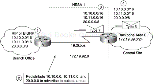
In this scenario, Router A is defined as an ASBR. It is configured to redistribute any routes within the RIP/EIGRP domain to the NSSA. When the area between the connecting routers is defined as an NSSA, the following happens:
Router A receives RIP or EIGRP routes for networks 10.10.0.0/16, 10.11.0.0/16, and 20.0.0.0/8.
Because Router A is also connected to an NSSA, it redistributes the RIP or EIGRP routers as Type 7 LSAs into the NSSA.
Router B, an ABR between the NSSA and the Backbone Area 0, receives the Type 7 LSAs.
After the SPF calculation on the forwarding database, Router B translates the Type 7 LSAs into Type 5 LSAs and then floods them throughout backbone Area 0. At this point, Router B could have summarized routes 10.10.0.0/16 and 10.11.0.0/16 as 10.0.0.0/8, or could have filtered one or more of the routes.
Type 7 LSAs have the following characteristics:
They are originated only by ASBRs connected between the NSSA and autonomous system domain.
They include a forwarding address field. This field is retained when a Type 7 LSA is translated as a Type 5 LSA.
They are advertised only within an NSSA.
They are not flooded beyond an NSSA. The ABR that connects to another nonstub area reconverts the Type 7 LSA into a Type 5 LSA before flooding it.
NSSA ABRs can be configured to summarize or filter Type 7 LSAs into Type 5 LSAs.
NSSA ABRs can advertise a Type 7 default route into the NSSA.
Type 7 LSAs have a lower priority than Type 5 LSAs; so when a route is learned with a Type 5 LSA and Type 7 LSA, the route defined in the Type 5 LSA will be selected first.
The steps used to configure OSPF NSSA are as follows:
Configure standard OSPF operation on one or more interfaces that will be attached to NSSAs.
Configure an area as NSSA using the following command:
router(config)#area area-id nssa
(Optional) Control the summarization or filtering during the translation. Figure3-15 shows how Router B will summarize routes using the following command:
           router(config)#summary-address prefix mask [not-advertise]
           [tag tag]
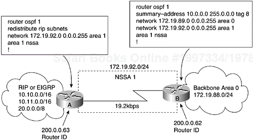
Be sure to evaluate these considerations before implementing NSSA. As shown in Figure3-15, you can set a Type 7 default route that can be used to reach external destinations. The command to issue a Type 7 default route is as follows:
router(config)#area area-id nssa [default-information-originate]
When configured, the router generates a Type 7 default into the NSSA by the NSSA ABR. Every router within the same area must agree that the area is NSSA; otherwise, the routers will not be able to communicate with one another.
If possible, avoid doing explicit redistribution on NSSA ABR because you could get confused about which packets are being translated by which router.
OSPF on-demand circuit is an enhancement to the OSPF protocol that allows efficient operation over on-demand circuits such as ISDN, X.25 SVCs, and dialup lines. This feature supports RFC 1793, "Extending OSPF to Support Demand Circuits." This RFC explains the operation of OSPF on-demand circuits. It has good examples and explains the operation of OSPF in this type of environment.
Prior to this feature, OSPF periodic Hello and LSA updates would be exchanged between routers that connected the on-demand link, even when there were no changes in the Hello or LSA information.
With OSPF on-demand circuit, periodic Hellos are suppressed and periodic refreshes of LSAs are not flooded over demand circuits. These packets bring up the links when they are exchanged for the first time only, or when there is a change in the information they contain. This operation allows the underlying data link layer to be closed when the network topology is stable, thus keeping the cost of the demand circuit to a minimum.
This feature is a standards-based mechanism similar to the Cisco Snapshot feature used for distance-vector protocols such as RIP.
This feature is useful when you want to have an OSPF backbone at the central site, and you want to connect telecommuters or branch offices to the central site. In this case, OSPF on-demand circuit allows the benefits of OSPF over the entire domain without excessive connection costs. Periodic refreshes of Hello updates and LSA updates, and other protocol overhead are prevented from enabling the on-demand circuit when there is no "real" data to transmit.
Overhead protocols such as Hellos and LSAs are transferred over the on-demand circuit upon initial setup only and when they reflect a change in the topology. This means that topology-critical changes that require new SPF calculations are transmitted to maintain network topology integrity, but that periodic refreshes that do not include changes are not transmitted across the link.
Figure3-16 shows the network that will form the basis for the following overview of OSPF on-demand circuit operation:
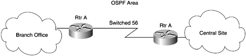
Upon initialization, Router A brings up the on-demand circuit to exchange Hellos and synchronize LSA databases with Router B. Because both routers are configured for OSPF on-demand circuit, each router's Hello packets and database description packets have the demand circuit (DC) bit set. As a result, both routers know to suppress periodic Hello packet updates. When each router floods LSAs over the network, the LSAs will have the DoNotAge (DNA) bit set. This means that the LSAs will not age. They can be updated if a new LSA is received with changed information, but no periodic LSA refreshes will be issued over the demand circuit.
When Router A receives refreshed LSAs for existing entries in its database, it will determine whether the LSAs include changed information. If not, Router A will update the existing LSA entries, but it will not flood the information to Router B. Therefore, both routers will have the same entries, but the entry sequence numbers may not be identical.
When Router A does receive an LSA for a new route or an LSA that includes changed information, it will update its LSA database, bring up the on-demand circuit, and flood the information to Router B. At this point, both routers will have identical sequence numbers for this LSA entry.
If there is no data to transfer while the link is up for the updates, the link is terminated.
When a host on either side needs to transfer data to another host at the remote site, the link will be brought up.
The steps used to configure OSPF on-demand circuit are summarized as follows:
Configure your on-demand circuit. For example:
           interface bri 0
           ip address 10.1.1.1 255.255.255.0
           encapsulation ppp
           dialer idle-timeout 3600
           dialer map ip name rtra 10.1.1.2 broadcast 1234
           dialer group 1
           ppp authentication chap
           dialer list 1 protocol ip permit
Enable OSPF operation, as follows:
router(config)#router ospf process-id
Configure OSPF on an on-demand circuit using the following interface command:
           interface bri 0
           ip ospf demand-circuit
If the router is part of a point-to-point topology, only one end of the demand circuit needs to be configured with this command, but both routers need to have this feature loaded. All routers that are part of a point-to-multipoint topology need to be configured with this command.
Consider the following before implementing OSPF on-demand circuit:
Because LSAs indicating topology changes are flooded over an on-demand circuit, you are advised to put demand circuits within OSPF stub areas or within NSSAs to isolate the demand circuits from as many topology changes as possible.
To take advantage of the on-demand circuit functionality within a stub area or NSSA, every router in the area must have this feature loaded. If this feature is deployed within a regular area, all other regular areas must also support this feature before the demand-circuit functionality can take effect. This is because external LSAs are flooded throughout all areas.
Do not enable this feature on a broadcast-based network topology because Hellos cannot be successfully suppressed, which means the link will remain up.
NBMA networks are those networks that support many (more than two) routers, but have no broadcast capability. Neighboring routers are maintained on these nets using OSPF's Hello protocol. Due to the lack of broadcast capability, however, some configuration information may be necessary to aid in the discovery of neighbors. On nonbroadcast networks, OSPF protocol packets that are normally multicast need to be sent to each neighboring router, in turn. An X.25 Public Data Network (PDN) is an example of a nonbroadcast network. Note the following:
OSPF runs in one of two modes over nonbroadcast networks. The first mode, called nonbroadcast multiaccess (NBMA), simulates the operation of OSPF on a broadcast network. The second mode, called point-to-multipoint, treats the nonbroadcast network as a collection of point-to-point links. Nonbroadcast networks are referred to as NBMA networks or point-to-multipoint networks, depending on OSPF's mode of operation over the network.
In NBMA mode, OSPF emulates operation over a broadcast network. A designated router is elected for the NBMA network, and the designated router originates an LSA for the network. The graph representation for broadcast networks and NBMA networks is identical.
NBMA mode is the most efficient way to run OSPF over nonbroadcast networks, both in terms of link-state database size and in terms of the amount of routing-protocol traffic. However, it has one significant restriction: It requires all routers attached to the NBMA network to be able to communicate directly. Although this restriction may be met on some nonbroadcast networks, such as an ATM subnet utilizing SVCs, it is often not met on other nonbroadcast networks, such as PVC-only Frame Relay networks.
On nonbroadcast networks in which not all routers can communicate directly, you can break the nonbroadcast network into logical subnets, with the routers on each subnet being able to communicate directly. Then, each separate subnet can be run as an NBMA network or a point-to-point network if each virtual circuit is defined as a separate logical subnet. This setup requires quite a bit of administrative overhead, however, and is prone to misconfiguration. It is probably better to run such a nonbroadcast network in point-to-multipoint mode.
Point-to-multipoint networks have been designed to work simply and naturally when faced with partial mesh connectivity. In point-to-multipoint mode, OSPF treats all router-to-router connections over the nonbroadcast network as if they were point-to-point links. No designated router is elected for the network, nor is there an LSA generated for the network. It may be necessary to configure the set of neighbors that are directly reachable over the point-to-multipoint network. Each neighbor is identified by its IP address on the point-to-multipoint network. Because no designated routers are elected on point-to-multipoint networks, the designated-router eligibility of configured neighbors is undefined.
Alternatively, neighbors on point-to-multipoint networks may be dynamically discovered by lower-level protocols such as Inverse ARP. In contrast to NBMA networks, point-to-multipoint networks have the following properties:
Adjacencies are established between all neighboring routers. There is no designated router or backup designated router for a point-to-multipoint network. No network LSA is originated for point-to-multipoint networks. Router priority is not configured for either point-to-multipoint interfaces or for neighbors on point-to-multipoint networks.
When originating a router LSA, point-to-multipoint interface is reported as a collection of "point-to-point links" to all the interface's adjacent neighbors, together with a single stub link advertising the interface's IP address with a cost of 0.
When flooding out a nonbroadcast interface (when in either NBMA or point-to-multipoint mode) the link-state update or link-state acknowledgment packet must be replicated in order to be sent to each of the interface's neighbors.
The following is an example of point-to-multipoint configuration on an NBMA (Frame Relay, in this case) network. Attached is the resulting routing table and router link state, along with other pertinent information:
  interface Ethernet0
   ip address 130.10.6.1 255.255.255.0
  !
  interface Serial0
   no ip address
   encapsulation frame-relay
   frame-relay lmi-type ansi
  !
  interface Serial0.1 multipoint
   ip address 130.10.10.3 255.255.255.0
   ip ospf network point-to-multipoint
   ip ospf priority 10
   frame-relay map ip 130.10.10.1 140 broadcast
   frame-relay map ip 130.10.10.2 150 broadcast
  !
  router ospf 2
   network 130.10.10.0 0.0.0.255 area 0
   network 130.10.6.0 0.0.0.255 area 1

  R6#sh ip ospf int s 0.1
  Serial0.1 is up, line protocol is up
  Internet Address 130.10.10.3/24, Area 0
  Process ID 2, Router ID 140.10.1.1, Network Type POINT_TO_MULTIPOINT, Cost: 6,
  Timer intervals configured, Hello 30, Dead 120, Wait 120, Retransmit 5
  Hello due in 00:00:18
  Neighbor Count is 2, Adjacent neighbor count is 2
  Adjacent with neighbor 130.10.10.2
  Adjacent with neighbor 130.10.5.129

  R6#sh ip ospf ne

  Neighbor ID      Pri     State     Dead Time      Address          Interface
  130.10.10.2       0     FULL/      00:01:37       130.10.10.2   Serial0.1
  130.10.5.129      0     FULL/      00:01:53       130.10.10.1   Serial0.1
  R6#

  R6#sh ip ro
  Codes: C - connected, S - static, I - IGRP, R - RIP, M - mobile, B - BGP
      D - EIGRP, EX - EIGRP external, O - OSPF, IA - OSPF inter area
      E1 - OSPF external type 1, E2 - OSPF external type 2, E - EGP
      i - IS-IS, L1 - IS-IS level-1, L2 - IS-IS level-2, * - candidate default
      U - per-user static route

  Gateway of last resort is not set

  130.10.0.0/16 is variably subnetted, 9 subnets, 3 masks
  O     130.10.10.2/32 [110/64] via 130.10.10.2, 00:03:28, Serial0.1
  C     130.10.10.0/24 is directly connected, Serial0.1
  O     130.10.10.1/32 [110/64] via 130.10.10.1, 00:03:28, Serial0.1
  O IA     130.10.0.0/22 [110/74] via 130.10.10.1, 00:03:28, Serial0.1
  O     130.10.4.0/24 [110/74] via 130.10.10.2, 00:03:28, Serial0.1
  C     130.10.6.0/24 is directly connected, Ethernet0

  R6#sh ip ospf data router 140.10.1.1

         OSPF Router with ID (140.10.1.1) (Process ID 2)
  Router Link States (Area 0)

   LS age: 806
   Options: (No TOS-capability)
   LS Type: Router Links
   Link State ID: 140.10.1.1
   Advertising Router: 140.10.1.1
   LS Seq Number: 80000009
   Checksum: 0x42C1
   Length: 60
   Area Border Router
    Number of Links: 3
  Link connected to: another Router (point-to-point)
   (Link ID) Neighboring Router ID: 130.10.10.2
   (Link Data) Router Interface address: 130.10.10.3
   Number of TOS metrics: 0
    TOS 0 Metrics: 64

  Link connected to: another Router (point-to-point)
   (Link ID) Neighboring Router ID: 130.10.5.129
   (Link Data) Router Interface address: 130.10.10.3
   Number of TOS metrics: 0
    TOS 0 Metrics: 64

  Link connected to: a Stub Network
   (Link ID) Network/subnet number: 130.10.10.3
   (Link Data) Network Mask: 255.255.255.255
   Number of TOS metrics: 0
    TOS 0 Metrics: 0
On-Demand Routing (ODR) is a mechanism that provides minimum-overhead IP routing for stub sites. The overhead of a general dynamic routing protocol is avoided, without incurring the configuration and management overhead of using static routing.
Astub router is the peripheral router in a hub-and-spoke network topology. Stub routers commonly have a WAN connection to the hub router and a small number of LAN network segments (stub networks) connected directly to the stub router. To provide full connectivity, the hub routers can be statically configured to know that a particular stub network is reachable via a specified access router. If there are multiple hub routers, many stub networks, or asynchronous connections between hubs and spokes, however, the overhead required to statically configure knowledge of the stub networks on the hub routers becomes too great.
On-Demand Routing allows stub routers to advertise their connected stub networks using CDP (Cisco Discovery Protocol).
ODR requires stub routers to be configured statically with default routes pointing to hub routers. The hub router is configured to accept remote stub networks via CDP. Once ODR is enabled on a hub router, the router begins installing stub network routes in the IP forwarding table. The hub router can also be configured to redistribute these routes into any configured dynamic IP routing protocols. No IP routing protocol is configured on the stub routers. With ODR, a router is automatically considered to be a stub when no IP routing protocols have been configured on it. The following is an ODR configuration command required on a hub router:
router odr
No configuration is required on the remote router because CDP is enabled by default.
The suggested Frame Relay configuration is point-to-point subinterface. Point-to-point subinterface configuration is used on the Frame Relay cloud because remote routers are configured with static defaults that point to the other end of the Frame Relay cloud—that is, the IP address of the hub router. When the PVC between the remote and the hub routers goes down, the point-to-point subinterface goes down and the static default route is no longer valid. If it is a multipoint configuration on the Frame Relay, the interface on the cloud does not go down when a PVC is inactive, and hence static default black holes the traffic.
The benefits of ODR are as follows:
ODR is a mechanism that provides minimum-overhead IP routing for stub sites. The overhead of a general dynamic routing protocol is avoided, without incurring the configuration and management overhead of using static routing.
ODR simplifies installation of IP stub networks in which the hub routers dynamically maintain routes to the stub networks. This is accomplished without requiring the configuration of an IP routing protocol at the stub routers. With ODR, the stub advertises IP prefixes corresponding to the IP networks configured on its directly connected interfaces. Because ODR advertises IP prefixes rather than IP network numbers, ODR can carry variable-length subnet mask (VLSM) information.
ODR minimizes the configuration and bandwidth overhead required to provide full routing connectivity. Moreover, it eliminates the need to configure an IP routing protocol at the stub routers.
You should consider the following when using ODR:
ODR propagates routes between routers using CDP. Therefore, ODR is partially controlled by the configuration of CDP. If CDP is disabled, the propagation of ODR routing information will cease.
By default, CDP sends updates every 60 seconds. This update interval may not be frequent enough to provide fast reconvergence. If faster convergence is required, the CDP update interval may need to be changed.
Limit of number of interfaces on the hub.
Recall the following design implications of EIGRP and OSPF:
Network topology
Addressing and route summarization
Route selection
Convergence
Network scalability
Security
This chapter also covered On-Demand Routing (ODR), a mechanism that provides minimum-overhead IP routing for stub sites. The overhead of a general dynamic routing protocol is avoided, without incurring the configuration and management overhead of using static routing. ODR minimizes the configuration and bandwidth overhead required to provide full routing connectivity. Moreover, it eliminates the need to configure an IP routing protocol at the stub routers.