
Chapter 4. The CUDA Execution Model
The heart of CUDA performance and scalability lies in the execution model and the simple partitioning of a computation into fixed-sized blocks of threads in the execution configuration. CUDA was created to map naturally the parallelism within an application to the massive parallelism of the GPGPU hardware. From the high-level language expression of the kernel to the replication of the lowest-level hardware units, on-board GPU scalability is preserved while many common parallel programming pitfalls are avoided. The result is massive thread scalability and high application performance across GPGPU hardware generations. The CUDA toolkit provides the programmer with those tools needed to exploit parallelism at both the thread level and the instruction level within the processing cores. Even the first CUDA program presented in Chapter 1 has the potential to run a million concurrent hardware threads of execution on some future generation of GPU. Meanwhile, the functor in Chapter 2 demonstrated high performance across multiple types and generations of GPUs.
Keywords
Execution model, Peak Performance, ILP (Instruction-level Parallelism), TLP (Thread-level parallelism), SM (Streaming Multiprocessor), teraflop
The heart of CUDA performance and scalability lies in the execution model and the simple partitioning of a computation into fixed-sized blocks of threads in the execution configuration. CUDA was created to map naturally the parallelism within an application to the massive parallelism of the GPGPU hardware. From the high-level language expression of the kernel to the replication of the lowest-level hardware units, on-board GPU scalability is preserved while many common parallel programming pitfalls are avoided. The result is massive thread scalability and high application performance across GPGPU hardware generations. The CUDA toolkit provides the programmer with those tools needed to exploit parallelism at both the thread level and the instruction level within the processing cores. Even the first CUDA program presented in Chapter 1 has the potential to run a million concurrent hardware threads of execution on some future generation of GPU. Meanwhile, the functor in Chapter 2 demonstrated high performance across multiple types and generations of GPUs.
At the end of this chapter, the reader will have a basic understanding of:
■ How CUDA expresses massive parallelism without imposing scaling limitations.
■ The meaning and importance of a warp and half-warp.
■ Scheduling, warp divergence, and why GPUs are considered a SIMT architecture.
■ How to use both TLP and ILP in a CUDA program.
■ The advantages and disadvantages of TLP and ILP for arithmetic and memory transactions.
■ The impact of warp divergence and general rules on how to avoid it.
■ The application of Little's law to streaming multiprocessors.
■ The nvcc compiler, SM related command-line options, and cuobjdump.
■ Those profiler measurements relevant to occupancy, TLP, ILP, and the SM.
GPU Architecture Overview
The heart of CUDA performance and scalability lies in the simple partitioning of a computation into fixed sized blocks of threads in the execution configuration. These thread blocks provide the mapping between the parallelism of the application and the massive replication of the GPGPU hardware.
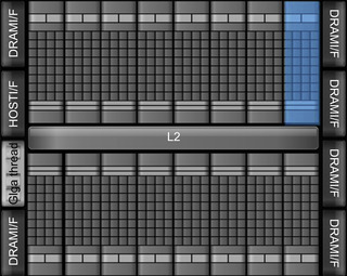
Massive GPU hardware parallelism is achieved through replication of a common architectural building block called a streaming multiprocessor (SM). By altering the number of SMs, GPU designers can create products to meet market needs at various price and performance points. The block diagram in Figure 4.1 illustrates the massive replication of multiprocessors on a GF100 (Fermi) series GPGPU.
The software abstraction of a thread block translates into a natural mapping of the kernel onto an arbitrary number of SM on a GPGPU. Thread blocks also act as a container of thread cooperation, as only threads in a thread block can share data. 1 Thus a thread block becomes both a natural expression of the parallelism in an application and of partitioning the parallelism into multiple containers that run independently of each other.
1For some problems and with good reason, a developer may choose to use atomic operations to communicate between threads of different thread blocks. This approach breaks the assumption of independence between thread blocks and may introduce programming errors, scalability, and performance issues.
The translation of the thread block abstraction is straightforward; each SM can be scheduled to run one or more thread blocks. Subject only to device limitations, this mapping:
■ Scales transparently to an arbitrary number of SM.
■ Places no restriction on the location of the SM (potentially allowing CUDA applications to transparently scale across multiple devices in the future).
■ Gives the hardware the ability to broadcast both the kernel executable and user parameters to the hardware. A parallel broadcast is the most scalable and generally the fastest communication mechanism that can move data to a large number of processing elements.
Because all the threads in a thread block execute on an SM, GPGPU designers are able to provide high-speed memory inside the SM called shared memory for data sharing. This elegant solution also avoids known scaling issues with maintaining coherent caches in multicore processors. A coherent cache is guaranteed to reflect the latest state of all the variables in the cache regardless of how many processing elements may be reading or updating a variable.
In toto, the abstraction of a thread block and replication of SM hardware work in concert to transparently provide unlimited and efficient scalability. The challenge for the CUDA programmer is to express their application kernels in such a way to exploit this parallelism and scalability.
Thread Scheduling: Orchestrating Performance and Parallelism via the Execution Configuration
Distributing work to the streaming multiprocessors is the job of the GigaThread global scheduler (highlighted in Figure 4.1). Based on the number of blocks and number of threads per block defined in the kernel execution configuration, this scheduler allocates one or more blocks to each SM. How many blocks are assigned to each SM depends on how many resident threads and thread blocks a SM can support.
NVIDIA categorizes their CUDA-enabled devices by compute capability. An important specification in the compute capability is the maximum number of resident threads per multiprocessor. For example, an older G80 compute capability 1.0 device has the ability to manage 768 total resident threads per multiprocessor. Valid block combinations for these devices include three blocks of 256 threads, six blocks of 128 threads, and other combinations not exceeding 768 threads per SM. A newer GF100, or compute capability 2.0 GPU, can support 1,536 resident threads or twice the number of a compute 1.0 multiprocessor.
The GigaThread global scheduler was enhanced in compute 2.0 devices to support concurrent kernels. As a result, compute 2.0 devices can better utilize the GPU hardware when confronted with a mix of small kernels or kernels with unbalanced workloads that stop using SM over time. In other words, multiple kernels may run at the same time on a single GPU as long as they are issued into different streams. Kernels are executed in the order in which they were issued and only if there are SM resources still available after all thread blocks for preceding kernels have been scheduled.
Each SM is independently responsible for scheduling its internal resources, cores, and other execution units to perform the work of the threads in its assigned thread blocks. This decoupled interaction is highly scalable, as the GigaThread scheduler needs to know only when an SM is busy.
On each clock tick, the SM warp schedulers decide which warp to execute next, choosing from those not waiting for:
■ Data to come from device memory.
■ Completion of earlier instructions.
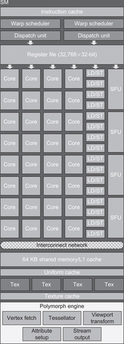
As illustrated in Figure 4.2, each GF100 SM has 32 SIMD (Single Instruction Multiple Data) cores. The use of a SIMD execution model means that the scheduler on the SM dictates that all the cores it controls will run the same instruction. Each core, however, may use different data. Basing the design of the streaming multiprocessors on a SIMD execution model is a beautiful example of “just enough and no more” in processor design because SIMD cores require less space and consume less power than non-SIMD designs. These benefits are multiplied by the massive replication of SM inside the GPU.
GPU hardware architects have been able to capitalize on the SIMD savings by devoting more power and space by adding ALU (Arithmetic and Logic Units), floating-point, and Special Function Units for transcendental functions. As a result, GPGPU devices have a high flop per watt ratio compared to conventional processors (Vuduc, 2010) as seen in Table 4.1.
To this point, we have correctly spoken about programming a GPU in terms of individual threads. From a performance perspective, it is necessary to start thinking in terms of the number of SIMD threads inside a warp or a half-warp on GF100 SM with dual schedulers. A warp is a block of 32 SIMD threads on most GPUs. Just like a thread block for the GigaThread scheduler, a warp is the basic unit for scheduling work inside a SM.
Because each warp is by definition a block of SIMD threads, the scheduler does not need to check for dependencies within the instruction stream. Figure 4.2 shows that each GF100 SM has two warp schedulers and two instruction dispatch units, which allows two warps to be issued and executed concurrently. Using this dual-issue model, GF100 streaming multiprocessors can achieve two operations per clock by selecting two warps and issuing one instruction from each warp to a group of sixteen cores, sixteen load/store units, or four SFUs.
Most instructions can be dual-issued: two integer instructions, two floating-point instructions, or a mix of integer, floating-point, load, store, and SFU instructions. For example:
■ The first unit can execute 16 FMA FP32s while the second concurrently processes 16 ADD INT32s, which appears to the scheduler as if they executed in one cycle.
■ The quadruple SFU unit is decoupled, and the scheduler can therefore send instructions to two SIMD units once it is engaged, which means that the SFUs and SIMD units can be working concurrently. This setup can provide a big performance win for applications that use transcendental functions.
GF100 GPUs do not support dual-dispatch of double-precision instructions, but a high IPC is still possible when running double-precision instructions because integer and other instructions can execute when double-precision operations are stalled waiting for data.
Utilizing a decoupled global and local scheduling mechanism based on thread blocks has a number of advantages:
■ It does not limit on-board scalability, as only the active state of the SMs must be monitored by the global scheduler.
■ Scheduling a thread block per SM limits the complexity of thread resource allocation and any interthread communication to the SM, which partitions each CUDA kernel in a scalable fashion so that no other SM or even the global scheduler needs to know what is happening within any other SM.
■ Future SM can be smarter and do more as technology and manufacturing improve with time.
Relevant computeprof Values for a Warp
| active warps/active cycle | The average number of warps that are active on a multiprocessor per cycle, which is calculated as: (active warps)/(active cycles) |
Warp Divergence
SIMD execution does have drawbacks, but it affects only code running inside an SM. GPGPUs are not true SIMD machines because they are composed of many SMs, each of which may be running one or more different instructions. For this reason, GPGPU devices are classified as SIMT (Single Instruction Multiple Thread) devices.
Programmers must be aware that conditionals (if statements) can greatly decrease performance inside an SM, as each branch of each conditional must be evaluated. Long code paths in a conditional can cause a 2-times slowdown for each conditional within a warp and a 2N slowdown for N nested loops. A maximum 32-time slowdown can occur when each thread in a warp executes a separate condition.
Fermi architecture GPUs utilize predication to run short conditional code segments efficiently with no branch instruction overhead. Predication removes branches from the code by executing both the if and else parts of a branch in parallel, which avoids the problem of mispredicted branches and warp divergence.
Section 6.2 of “The CUDA C Best Practices Guide” notes:
When using branch predication, none of the instructions whose execution depends on the controlling condition is skipped. Instead, each such instruction is associated with a per-thread condition code or predicate that is set to true or false according to the controlling condition. Although each of these instructions is scheduled for execution, only the instructions with a true predicate are actually executed. Instructions with a false predicate do not write results, and they also do not evaluate addresses or read operands. (NVIDIA, CUDA C Best Practices Guide, May 2011, p. 56)
The code in Example 4.1, “A Short Code Snippet Containing a Conditional,” contains a conditional that would run on all threads computing the logical predicate and two predicated instructions as shown in Example 4.2:
if (x<0.0) z = x−2.0;
else z = sqrt(x);
The sqrt has a false predicate when x < 0 so no error occurs from attempting to take the square root of zero.
p = (x<0.0);// logical predicate
p: z = x−2.0;// True predicated instruction
!p: z = sqrt(x); // False predicated instruction
Per section 6.2 of “The CUDA C Best Practices Guide,” the length of the predicated instructions is important:
The compiler replaces a branch instruction with predicated instructions only if the number of instructions controlled by the branch condition is less than or equal to a certain threshold: If the compiler determines that the condition is likely to produce many divergent warps, this threshold is 7; otherwise it is 4. (NVIDIA, CUDA C Best Practices Guide, May 2011, p. 56)
If the code in the branches is too long, the nvcc compiler inserts code to perform warp voting to see if all the threads in a warp take the same branch. If all the threads in a warp vote the same way, there is no performance slowdown.
In some cases, the compiler can determine at compile time that all the threads in the warp will go the same way. In Example 4.3, “Example When Voting Is Not Needed,” there is no need to vote even though case is a nonconstant variable:
//The variable case has the same value across all threads
if (case==1)
z = x*x;
else
z = x+2.3;
Guidelines for Warp Divergence
Sometimes warp divergence is unavoidable. Common application examples include PDEs (Partial Differential Equations) with boundary conditions, graphs, trees, and other irregular data structures. In the worst case, a 32-time slowdown can occur when:
■ One thread needs to perform an expensive computational task.
■ Each thread performs a separate task.
Avoiding warp divergence is a challenge. Though there are many possible solutions, none will work for every situation. Following are some guidelines:
■ Try to reformulate the problem to use a different algorithm that either does not cause warp divergence or expresses the problem so that the compiler can reduce or eliminate warp divergence.
■ Consider creating separate lists of expensive vs. inexpensive operations and using each list in a separate kernel. Hopefully, the bulk of the work will occur in the inexpensive kernel. Perhaps some of the expensive work can be performed on the CPU.
■ Order the computation (or list of computations) to group computations into blocks that are multiples of a half-warp.
■ If possible, use asynchronous kernel execution to exploit the GPU SIMT execution model.
■ Utilize the host processor(s) to perform part of the work that would cause a load imbalance on the GPU.
The book GPU CUDA Gems (Hwu, 2011) is a single-source reference to see how many applications handle problems with irregular data structures and warp divergence. Each chapter contains detailed descriptions of the problem, solutions, and reported speedups. Examples include:
■ Conventional and novel approaches to accelerate an irregular tree-based data structure on GPGPUs.
■ Avoiding conditional operations that limit parallelism in a string similarity algorithm.
■ Using GPUs to accelerate a dynamic quadrature grid method and avoid warp divergence as grid points move over the course of the calculation.
■ Approached to irregular meshes that involve conditional operations and approaches to regularize computation.
Relevant computeprof Values for Warp Divergence
| Divergent branches (%) | The percentage of branches that are causing divergence within a warp amongst all the branches present in the kernel. Divergence within a warp causes serialization in execution. This is calculated as: (100 * divergent branch)/(divergent branch + branch) |
| Control flow divergence (%) | Control flow divergence gives the percentage of thread instructions that were not executed by all threads in the warp, hence causing divergence. This should be as low as possible. This is calculated as: 100 * ((32 * instructions executed)—threads instruction executed)/(32 * instructions executed)) |
Warp Scheduling and TLP
Running multiple warps per SM is the only way a GPU can hide both ALU and memory latencies to keep the execution units busy.
From a software perspective, the hardware SM scheduler is fast enough that it basically has no overhead. Inside the SM, the hardware can detect those warps whose next instruction is ready to run because all resource and data dependencies have been resolved. From this pool of eligible warps, the SM scheduler selects one based on an internal prioritized schedule. It then issues the instruction from that warp to the SIMD cores. If all the warps are stalled, meaning they all have some unresolved dependency, then no instruction can be issued resulting in idle hardware and decreased performance.
The idea behind TLP is to give the scheduler as many threads as possible to choose from to minimize the potential for a performance loss. Occupancy is a measure of TLP, which is defined as the number of warps running concurrently on a multiprocessor divided by maximum number of warps that can be resident on an SM. A high occupancy implies that the scheduler on the SM has many warps to choose from and thus hide both ALU and data latencies. Chances are at lease one warp should be ready to run because all the dependencies are resolved.
Though simple in concept, occupancy is complicated in practice, as it can be limited by on-chip SM memory resources such as registers and shared memory. NVIDIA provides the CUDA Occupancy calculator to help choose execution configurations.
Common execution configuration (block per grid) heuristics include:
■ Specify more blocks than number of SM so all the multiprocessors have at least one block to execute.
■ This is a lower bound, as specifying fewer blocks than SM will clearly not utilize all the resources of the GPU.
■ To exploit asynchronous kernel execution for small problems, the developer may purposely underutilize the GPU. GF100 and later architectures can utilize concurrent kernel execution to increase application performance by running blocks from different kernels on unused SM. These GPUs accelerate those applications that have multiple kernels that are too small to run on all the SM of the GPU but take too much time to export to the host processor.
■ Specify multiple blocks per SM to run concurrently inside a SM.
■ Choose the number of blocks to be a multiple of the number of SM on the GPU to fully utilize all the SM. This approach ensures that all the SM have a balanced workload.
■ Blocks that are not waiting at a __syncthreads will keep the hardware busy.
■ The numbers of blocks that can run are subject to resource availability on the SM including register and shared memory space.
■ When possible, specify a very large number of blocks per grid (e.g., thousands).
■ Doing so will help the application across multiple GPGPU generations.
■ It will also keep the SM fully loaded with resident thread blocks.
Relevant computeprof Values for Occupancy
| Achieved kernel occupancy | This ratio provides the actual occupancy of the kernel based on the number of warps executing per cycle on the SM. It is the ratio of active warps and active cycles divided by the max number of warps that can execute on an SM. This is calculated as: (active warps/active cycles)/4 |
ILP: Higher Performance at Lower Occupancy
High occupancy does not necessarily translate into the fastest application performance. Instruction-level parallelism (ILP) can be equally effective in hiding arithmetic latency by keeping the SIMD cores busy with fewer threads that consume fewer resources and introduce less overhead.
The reasoning for ILP is simple and powerful: using fewer threads means that more registers can be used per thread. Registers are a precious resource, as they are the only memory fast enough to attain peak GPU performance. The larger the bandwidth gap between the register store and other memory, the more data that must come from registers to achieve high performance.
Sometimes having a few more registers per thread can prevent register spilling and preserve high performance. Although necessary, register spilling violates the programmer's expectation of high performance from register memory and can cause catastrophic performance decreases. Utilizing fewer threads also benefit kernels that use shared memory by reducing the number of shared memory accesses and by allowing data reuse within a thread (Volkov, 2010). A minor benefit includes a reduction in some of the work that the GPU must perform per thread.
The following loop, for example, would consume 2048 bytes of register storage and require that the loop counter, i, be incremented 512 times in a block with 512 threads. A thread block containing only 64 threads would require only 256 bytes of register storage and reduce the number of integer increment in place operations by a factor of 4. See Example 4.4, “Simple for Loop to Demonstrate ILP Benefits”:
for(int i=0; i < n; i++) ...
Reading horizontally across the columns, Table 4.2 encapsulates how the number of registers per threads increases as the occupancy decreases for various compute generations.
ILP Hides Arithmetic Latency
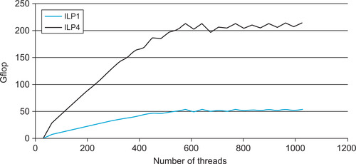
As with TLP, multiple threads provide the needed parallelism. For example, the shaded row in Figure 4.3 highlights four independent operations that happen in parallel across three threads.
| Thread 1 | Thread 2 | Thread 3 | Thread 4 |
|---|---|---|---|
| x = x + c | y = y + c | z = z + c | w = w + c |
| x = x + b | y = y + b | z = z + b | w = w + b |
| x = x + a | y = y + a | z = z + a | w = w + a |
Due to warp scheduling, parallelism can also happen among the instructions within a thread, as long as there are enough threads to create two or more warps within a block.
| Thread | ||
|---|---|---|
| Instructions -> | w = w + b | Four independent operations |
| z = z + b | ||
| y = y + b | ||
| x = x + b | ||
| w = w + a | Four independent operations | |
| z = z + a | ||
| y = y + a | ||
| x = x + a |
The following example demonstrates ILP by creating two or more warps that run on a single SM. As can be seen in Example 4.5, “Arithmetic ILP Benchmark,” the execution configuration specifies only one block. The number of warps resident on the SM is increased as the number of threads within the block is increased from 32 to 1024, and the performance is reported. This example will run to completion on a compute 2.0 device that can support 1024 threads per block. Earlier devices will detect a runtime error via the call to cudaGetLastError, which will stop the test when the maximum number of threads per block exceeds the number that the GPU can support. Because kernel launches are asynchronous, cudaSynchronizeThread is used to wait for kernel completion.
#include <omp.h>
#include <iostream>
using namespace std;
#include <cmath>
//create storage on the device in gmem
__device__ float d_a[32], d_d[32];
__device__ float d_e[32], d_f[32];
#define NUM_ITERATIONS ( 1024 * 1024)
#ifdef ILP4
// test instruction level parallelism
#define OP_COUNT 4*2*NUM_ITERATIONS
__global__ void kernel(float a, float b, float c)
{
register float d=a, e=a, f=a;
#pragma unroll 16
for(int i=0; i < NUM_ITERATIONS; i++) {
a = a * b + c;
d = d * b + c;
e = e * b + c;
f = f * b + c;
}
// write to gmem so the work is not optimized out by the compiler
d_a[threadIdx.x] = a; d_d[threadIdx.x] = d;
d_e[threadIdx.x] = e; d_f[threadIdx.x] = f;
}
#else
// test thread level parallelism
#define OP_COUNT 1*2*NUM_ITERATIONS
__global__ void kernel(float a, float b, float c)
{
#pragma unroll 16
for(int i=0; i < NUM_ITERATIONS; i++) {
a = a * b + c;
}
// write to gmem so the work is not optimized out by the compiler
d_a[threadIdx.x] = a;
}
#endif
int main()
{
// iterate over number of threads in a block
for(int nThreads=32; nThreads <= 1024; nThreads += 32) {
double start=omp_get_wtime();
kernel<<<1, nThreads>>>(1., 2., 3.); // async kernel launch
if(cudaGetLastError() != cudaSuccess) {
cerr << "Launch error" << endl;
return(1);
}
cudaThreadSynchronize(); // need to wait for the kernel to complete
double end=omp_get_wtime();
cout << "warps" << ceil(nThreads/32) << " "
<< nThreads << " " << (nThreads*(OP_COUNT/1.e9)/(end - start))
<< " Gflops " << endl;
}
return(0);
}
As seen in Figure 4.3, ILP increases performance just by increasing the number of independent instructions per thread. The best performance on a compute 2.0 device occurs when 576 threads are resident on the SM. As noted in the presentation “Better Performance at Lower Occupancy,” the upper bound currently appears to be an ILP of 4 (Volkov, 2010). It is suspected that the scoreboard on the SM that tracks memory usage is the limiting factor. The patent “Tracking Register Usage During Multithreaded Processing Using a Scoreboard” (Coon, Mills, Oberman, & Siu, 2008) might provide additional insight.
Table 4.5 shows the minimum arithmetic parallelism needed to achieve 100 percent throughput (Volkov, 2010).
ILP Hides Data Latency
It is important to note that threads don't stall in the SM on a memory access—only on data dependencies. From the perspective of a warp, a memory access requires issuing a load or store instruction to the LD/ST units. 2 The warp can then continue issuing other instructions until it reaches one that depends on the completion of a memory transaction. At that point, the warp will stall. To increase performance, the compiler can reorder instructions to:
2Although there is no difference in performing a store or load operation, the literature discusses ILP writes in terms of multiple outputs—meaning multiple write operations to memory.
■ Keep the largest number of memory transactions “in flight” and thus best utilize memory bandwidth and the LD/ST units.
■ Supply other, nondependent instructions required by the thread to keep the computational cores busy.
■ Minimize the time that dependent instructions must remain in the queue by positioning the data-dependent instruction in the queue so that it reaches the top of the queue close to the expected data arrival time.
As a result of this complex choreography, ILP can also hide memory latency. Vasily Volkov notes that ILP can achieve 84 percent of peak memory bandwidth while requiring only 4 percent occupancy when copying 14 float4 values per thread (Volkov, 2010). A float4 is a structure of four 32-bit floating-point variables that fits perfectly into a 128-bit cache line. These structures exploit the bit-level parallelism of a cache line memory transaction as well as ILP parallelism.
ILP in the Future
The current GF100 architecture encourages the use of smaller blocks because it can schedule more blocks due to the additional resources per SM. This approach presents a new way of thinking about problems to achieve both high utilization and performance. It is worth noting that compute 2.0 devices and even 1.x GPUs can sometimes issue a second instruction from the same warp in parallel to the special function unit.
CPU developers will recognize ILP as a form of superscalar execution that executes more than one instruction during a clock cycle by simultaneously dispatching multiple instructions to redundant functional units on the processor. NVIDIA has added superscalar execution to the scheduler in compute 2.1 devices. The warp scheduler in these devices has the ability to analyze the next instruction in a warp to determine if that instruction is ILP-safe and whether there is an execution unit available to handle it. The result is that compute 2.1 devices can execute a warp in a superscalar fashion for any CUDA code without requiring explicit programmer actions to force ILP.
ILP has been incorporated into the CUBLAS 2.0 and CUFFT 2.3 libraries. Performing an single-precision level-3 BLAS matrix multiply (SGEMM) on two large matrices demonstrates the following performance increases (Volkov, 2010):
Similarly, ILP benefits batched 1024-point complex-to-complex single-precision Fast Fourier Transform (FFTs):
ILP benefits arithmetic problems: Current work on the MAGMA BLAS libraries demonstrates up to 838 Gflop/s using 33 percent occupancy and 2 thread blocks per SM (Volkov, 2010). The MAGMA team has made the conclusion that dense linear algebra methods are now a better fit on GPU architectures instead of traditional multicore architectures (Nath, Stanimire, & Dongerra, 2010).
ILP benefits memory bandwidth problems: To saturate the bus on a Fermi C2050 requires keeping 30–50 128-byte transactions in flight per SM (Micikevicius, 2010). Volkov recommends keeping 100 KB in flight to hide memory latency—less if the kernel is compute-bound.
Relevant computeprof Values for Instruction Rates
| Instruction throughput | This value is the ratio of achieved instruction rate to peak single-issue instruction rate. The achieved instruction rate is calculated using the profiler counter “instructions.” The peak instruction rate is calculated based on the GPU clock speed. In the case of instruction dual-issue coming into play, this ratio shoots up to greater than 1. This is calculated as: (instructions)/(gpu_time * clock_frequency) |
| Ideal instruction/byte ratio | This value is a ratio of the peak instruction throughput and the peak memory throughput of the CUDA device. This is a property of the device and is independent of the kernel. |
| Instruction/byte | This value is the ratio of the total number of instructions issued by the kernel and the total number of bytes accessed by the kernel from global memory. If this ratio is greater than the ideal instruction/byte ratio, then the kernel is compute-bound, and if it's less, then the kernel is memory-bound. This is calculated as: (32 * instructions issued * #SM)/{32 * (l2 read requests + l2 write requests + l2 read texture requests)} |
| IPC (instructions per cycle) | This value gives the number of instructions issued per cycle. This should be compared to maximum IPC possible for the device. The range provided is for single-precision floating-point instructions. This is calculated as: (instructions issued/active cycles) |
| Replayed instructions (%) | This value gives the percentage of instructions replayed during kernel execution. Replayed instructions are the difference between the numbers of instructions that are actually issued by the hardware to the number of instructions that are to be executed by the kernel. Ideally, this should be zero. This is calculated as: 100 * (instructions issued—instruction executed)/instruction issue |
Little's Law
Little's law (Little, 1961) is derived from general information theory but has important application to understanding the performance of memory hierarchies. Generalized to multiprocessor systems, Little's law for concurrency (Equation 4.1) can be expressed as:
(4.1)
Nearly all CUDA applications will be limited by memory bandwidth. The performance of global memory is of particular concern, as can be seen in the bandwidths reported in “Better Performance at Lower Occupancy” (Volkov, 2010):
■ Register memory (≈8 TB/s)
■ Shared memory (≈1.6 TB/s)
■ Global memory (177 GB/s)
From a TLP point of view, Little's law tells us that the number of memory transactions “in flight,” N (see Equation 4.2, “TLP memory transactions in flight”), is the product of the arrival rate λ and the memory latency, L.
(4.2)
In other words, as additional threads are added and multiplexed over the same hardware resources, greater latency can be hidden. As we have observed, this is an overly simplistic view, as complex data dependencies introduce stalls plus hardware limitations create bottlenecks.
From an ILP point of view, independent memory transactions can be batched (Equation 4.3, “ILP-batched memory transactions in flight”).
(4.3)
Saturating the bus on a Fermi C2050 requires keeping 30–50 128-byte transactions in flight per SM (Micikevicius, 2010). Volkov recommends the minimum parallelism for peak arithmetic performance on a C2050 be 576 threads per block and keeping 100 KB of data in flight for peak memory performance on memory-bound kernels. Table 4.8 summarizes these results.
| Latency | Throughput | Parallelism | |
|---|---|---|---|
| Arithmetic | ≈18 | 32 | ≈576 |
| Memory | <800 cycles | <177 GB.s | <100 KB |
To increase the concurrency in your applications, consider the following:
■ Increase occupancy.
■ Maximize the available registers using the nvcc command-line option -maxrregcount, or giving the compiler additional per kernel help with the __launch_bounds__ specification in the kernel declaration.
■ Adjust the thread block dimensions to best utilize the SM warp scheduler(s).
■ Modify the code to use ILP and process several elements per thread.
■ Pay careful attention to the instruction “mix”:
■ For example, the math-to-memory operation ratios.
■ Don't bottleneck on one function unit causing the other units to stall.
■ Don't “traffic-jam” kernel code:
■ Try to create lots of small thread blocks containing a uniform distribution of operation densities (e.g., int, floating-point, memory, and SFU).
■ Don't bunch operations of a similar type in one section of a kernel, as doing so could cause a load imbalance in the SM.
CUDA Tools to Identify Limiting Factors
CUDA provides several tools to work with your code and the concurrency of your kernels.
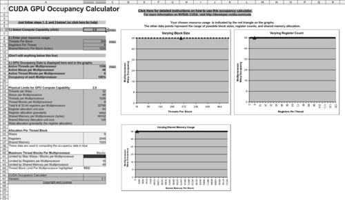
The CUDA Occupancy Calculator is a good tool to use during the planning stages to understand occupancy across devices. As shown in Figure 4.4, “Screenshot of the CUDA Occupancy Calculator,” this is a spreadsheet that the programmer can use to ask “what if” questions based on register and shared memory usage.
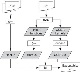
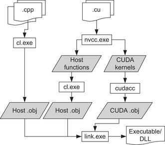
The nvcc Compiler
The nvcc compiler provides a common compilation framework for the UNIX, Windows, and Mac OS X operating systems.
As shown in Example 4.5, the nvcc compiler provides the #pragma unroll directive, which can be used to control unrolling of any given loop. It must be placed immediately before the loop and applies only to that loop. By default, the compiler unrolls small loops with a known trip count. If the loop is large or the trip count cannot be determined, the user can specify how many times the loop is to be unrolled.
The #pragma unroll 16 used in Example 4.5 tells the compiler to unroll the loop 16 times to prevent the control logic of the for loop from interfering with the ILP test results.
The primary benefits gained from loop unrolling are:
■ Reduced dynamic instruction count due to fewer number of compare and branch operations for the same amount of work done.
■ Better scheduling opportunities due to the availability of additional independent instructions can improve ILP plus hide pipeline and memory access latencies.
■ Opportunities for exploiting register and memory hierarchy locality when outer loops are unrolled and inner loops are fused (unroll-and-jam transformation).
Loop unrolling is not a panacea, as it can degrade performance due to excessive register usage and spilling to local memory.
The following nvcc command-line switches are also important for optimization and code generation:
■ -arch=sm_20 generates code for compute 2.0 devices.
■ -maxrregcount=N specifies the maximum number of registers kernels can use at a per-file level.
■ The __launch_bounds__ qualifier can be inserted in the declaration of the kernel as shown in Example 4.6 to control the number of registers on a per-kernel basis.
■ --ptxas-options=-v or -Xptxas=-v lists per-kernel register, shared, and constant memory usage.
■ -use_fast_math coerces every functionName() call to the equivalent native hardware function call name, __functionName(). This approach makes the code run faster at the cost of slightly diminished precision and accuracy.
Launch Bounds
Controlling register usage is key to achieving high performance in CUDA. To minimize register usage, the compiler utilizes a set of heuristics. A heuristic is a rule-of-thumb guideline generally derived from observation and trial and error.
The developer can aid the compiler through the use of a __launch_bounds__ qualifier in the definition of a __global__ function as shown in Example 4.6, “Example Launch Bounds Usage” where:
__global__ void
__launch_bounds__ (maxThreadsPerBlock, minBlocksPerMultiprocessor)
kernel(float a, float b, float c)
{
...
}
■ maxThreadsPerBlock specifies the maximum number of threads per block with which the application will use.
■ minBlocksPerMultiprocessor is optional and specifies the desired minimum number of resident blocks per multiprocessor. It compiles to the .minnctapersm PTX directive.
If launch bounds are specified, the compiler has the opportunity to increase register usage to better hide instruction latency. A kernel will fail to launch if the execution configuration specifies more threads per block than allowed by the launch bounds directive.
The Disassembler
The cuobjdump disassembler is a useful tool to examine the instructions generated by the compiler. It can be utilized to examine the mix of instructions provided in a warp to the SM as well as checking on what the compiler is doing. Example 4.7, “cuobjdump without loop unrolling,” is the code for Example 4.5 without loop unrolling. The bold code shows that only one fused mult-add (FFMA) instruction is utilized.
code for sm_20
Function : _Z6kernelfff
/*0000*//*0x00005de428004404*/MOV R1, c [0x1] [0x100];
/*0008*//*0x80001de428004000*/MOV R0, c [0x0] [0x20];
/*0010*//*0xfc009de428000000*/MOV R2, RZ;
/*0018*//*0x04209c034800c000*/IADD R2, R2, 0x1;
/*0020*//*0x9000dde428004000*/MOV R3, c [0x0] [0x24];
/*0028*//*0x0421dc231a8e4000*/ISETP.NE.AND P0, pt, R2, c [0x10] [0x0], pt;
/*0030*//*0xa0301c0030008000*/FFMA R0, R3, R0, c [0x0] [0x28];
/*0038*//*0x600001e74003ffff*/@P0 BRA 0x18;
/*0040*//*0x84009c042c000000*/S2R R2, SR_Tid_X;
/*0048*//*0x0000dde428007800*/MOV R3, c [0xe] [0x0];
/*0050*//*0x10211c032007c000*/IMAD.U32.U32 R4.CC, R2, 0x4, R3;
/*0058*//*0x10209c435000c000*/IMUL.U32.U32.HI R2, R2, 0x4;
/*0060*//*0x10215c4348007800*/IADD.X R5, R2, c [0xe] [0x4];
/*0068*//*0x00401c8594000000*/ST.E [R4], R0;
/*0070*//*0x00001de780000000*/EXIT;
..........................
The impact of the loop unrolling can be seen in Example 4.8, “cuobjdump showing loop unrolling,” through the replication of the FFMA instruction:
code for sm_20
Function : _Z6kernelfff
/*0000*//*0x00005de428004404*/MOV R1, c [0x1] [0x100];
/*0008*//*0x80001de428004000*/MOV R0, c [0x0] [0x20];
/*0010*//*0xfc009de428000000*/MOV R2, RZ;
/*0018*//*0x9000dde428004000*/MOV R3, c [0x0] [0x24];
/*0020*//*0x40209c034800c000*/IADD R2, R2, 0x10;
/*0028*//*0xa0301c0030008000*/FFMA R0, R3, R0, c [0x0] [0x28];
/*0030*//*0x0421dc231a8e4000*/ISETP.NE.AND P0, pt, R2, c [0x10] [0x0], pt;
/*0038*//*0xa0301c0030008000*/FFMA R0, R3, R0, c [0x0] [0x28];
/*0040*//*0xa0301c0030008000*/FFMA R0, R3, R0, c [0x0] [0x28];
/*0048*//*0xa0301c0030008000*/FFMA R0, R3, R0, c [0x0] [0x28];
/*0050*//*0xa0301c0030008000*/FFMA R0, R3, R0, c [0x0] [0x28];
/*0058*//*0xa0301c0030008000*/FFMA R0, R3, R0, c [0x0] [0x28];
/*0060*//*0xa0301c0030008000*/FFMA R0, R3, R0, c [0x0] [0x28];
/*0068*//*0xa0301c0030008000*/FFMA R0, R3, R0, c [0x0] [0x28];
/*0070*//*0xa0301c0030008000*/FFMA R0, R3, R0, c [0x0] [0x28];
/*0078*//*0xa0301c0030008000*/FFMA R0, R3, R0, c [0x0] [0x28];
/*0080*//*0xa0301c0030008000*/FFMA R0, R3, R0, c [0x0] [0x28];
/*0088*//*0xa0301c0030008000*/FFMA R0, R3, R0, c [0x0] [0x28];
/*0090*//*0xa0301c0030008000*/FFMA R0, R3, R0, c [0x0] [0x28];
/*0098*//*0xa0301c0030008000*/FFMA R0, R3, R0, c [0x0] [0x28];
/*00a0*//*0xa0301c0030008000*/FFMA R0, R3, R0, c [0x0] [0x28];
/*00a8*//*0xa0301c0030008000*/FFMA R0, R3, R0, c [0x0] [0x28];
/*00b0*//*0x800001e74003fffd*/@P0 BRA 0x18;
/*00b8*//*0x84009c042c000000*/S2R R2, SR_Tid_X;
/*00c0*//*0x0000dde428007800*/MOV R3, c [0xe] [0x0];
/*00c8*//*0x10211c032007c000*/IMAD.U32.U32 R4.CC, R2, 0x4, R3;
/*00d0*//*0x10209c435000c000*/IMUL.U32.U32.HI R2, R2, 0x4;
/*00d8*//*0x10215c4348007800*/IADD.X R5, R2, c [0xe] [0x4];
/*00e0*//*0x00401c8594000000*/ST.E [R4], R0;
/*00e8*//*0x00001de780000000*/EXIT;
..........................
As of CUDA 4.0, the nvcc compiler has the ability to include inline PTX assembly language. PTX is the low-level parallel thread execution virtual machine and instruction set architecture (ISA). The most current information on PTX can be found in the document “PTX: Parallel Thread Execution ISA” that is included with each release.
PTX Kernels
Giving developers the ability to disassemble and create assembly language kernels provides everything an adventurous programmer needs to directly program the SM on a GPU. The PTX kernel in Example 4.9 was taken from the NVIDIA ptxjit sample provided with the SDK samples:
/*
* PTX is equivalent to the following kernel:
*
* __global__ void myKernel(int *data)
* {
*int tid = blockIdx.x * blockDim.x + threadIdx.x;
*data[tid] = tid;
* }
*
*/
char myPtx[] = "
.version 1.4
.target sm_10, map_f64_to_f32
.entry _Z8myKernelPi (
.param .u64 __cudaparm__Z8myKernelPi_data)
{
.reg .u16 %rh<4>;
.reg .u32 %r<5>;
.reg .u64 %rd<6>;
cvt.u32.u16%r1, %tid.x;
mov.u16%rh1, %ctaid.x;
mov.u16%rh2, %ntid.x;
mul.wide.u16%r2, %rh1, %rh2;
add.u32%r3, %r1, %r2;
ld.param.u64%rd1, [__cudaparm__Z8myKernelPi_data];
cvt.s64.s32%rd2, %r3;
mul.wide.s32%rd3, %r3, 4;
add.u64%rd4, %rd1, %rd3;
st.global.s32[%rd4+0], %r3;
exit;
}
";
GPU Emulators
GPU simulators such as ocelot have unique abilities to characterize the runtime behavior of CUDA kernels code that are not available to other tools in the GPU toolchain (Farooqui, Kerr, Diamos, Yalamanchili, & Schwan, 2011). Features include:
■ Workload characterization
■ Load imbalance
■ “Hot-spots” in the PTX code
The ocelot tool that can be freely downloaded.
Summary
Understanding the SM is the key to understanding GPGPU programming. The twin concepts of a thread block and warp of SIMD threads encompass the scalability, performance, and power efficiency of GPU computing. Knowing how instructions execute in parallel within an SM, as well as the factors that stall the instruction pipeline, is fundamental to understanding GPGPU application performance. Little's law, and queuing theory in general, provide the theoretical foundation upon which very detailed GPU and application models can be based. Empirical studies have shown that exploiting both ILP and TLP provides the highest application performance. The benefits have been so significant that both ILP and TLP are now utilized in the CUBLAS and CUFFT libraries, which are the keystone of many applications.
Knowledgeable CUDA programmers have the ability to incorporate both ILP and TLP in their applications. NVIDIA has provided the necessary tools so that UNIX, Windows, and Mac OS X developers can examine, experiment with, and alter the instruction mix in their kernels to best exploit ILP and capture TLP with controlled register usage. Exploiting these tools can make the difference between good and great performance. Similarly, understanding and avoiding warp divergence can make all the difference when programming with irregular data structures or for applications that have irregular boundaries.
..................Content has been hidden....................
You can't read the all page of ebook, please click here login for view all page.