
Chapter 2. CUDA for Machine Learning and Optimization
GPGPUs are powerful tools that are well-suited to unraveling complex real-world problems. Using only the simple CUDA capabilities introduced in Chapter 1, this chapter demonstrates how to greatly accelerate nonlinear optimization problems using the derivative-free Nelder-Mead and Levenberg-Marquardt optimization algorithms. Single- and double-precision application performance will be measured and compared between an Intel Xeon e5630 processor and an NVIDIA C2070 GPU as well as an older 10-series NVIDIA GTX 280 gaming GPU. Working example code is provided that can train the classic nonlinear XOR machine-learning problem 85 times faster than a modern quad-core Intel Xeon processor (341 times faster than single-core performance) under Linux with comparable performance under Windows 7.
Keywords
Functor, Machine learning, Order of Magnitude, Optimization, Computational universal, Nelder-Mead, Levenburg-Marquardt, Curse of dimensionality, neural network
GPGPUs are powerful tools that are well-suited to unraveling complex real-world problems. Using only the simple CUDA capabilities introduced in Chapter 1, this chapter demonstrates how to greatly accelerate nonlinear optimization problems using the derivative-free Nelder-Mead and Levenberg-Marquardt optimization algorithms. Single- and double-precision application performance will be measured and compared between an Intel Xeon e5630 processor and an NVIDIA C2070 GPU as well as an older 10-series NVIDIA GTX 280 gaming GPU. Working example code is provided that can train the classic nonlinear XOR machine-learning problem 85 times faster than a modern quad-core Intel Xeon processor (341 times faster than single-core performance) under Linux with comparable performance under Windows 7.
At the end of the chapter, the reader will have a basic understanding of:
■ Two popular optimization techniques, including GPU scalability limitations of the Levenberg-Marquardt algorithm
■ How a CUDA-literate programmer can make significant contributions to modeling and data-mining efforts
■ Machine learning and why the XOR problem is important to computationally universal devices
■ C++ functors and how to write a single Thrust functor using __host__ and __device__ qualifiers that can run on both host and GPGPU devices
■ Some example programs that demonstrate orders-of-magnitude increased performance over a conventional processor on techniques that can be applied to problems in machine learning, signal processing, statistics, and many other fields
Modeling and Simulation
Mathematical modeling and numerical simulation are two important, distinct, and closely linked aspects of applied mathematics. A mathematical model is an abstraction of reality that can be used for analysis and prediction. Numerical simulation is based on applications that map mathematical models onto the computer. In combination, modeling and simulation are powerful techniques to advance human understanding of complex phenomena.
This book does not attempt to duplicate or shed new insight on the tremendous volume of work that has already been published concerning modeling and simulation. Depending on your particular area of interest, there are a number of excellent texts available that provide both precise and detailed introductions. Our focus is to provide the tools needed to exploit massively parallel hardware with CUDA so that readers can make their own contributions in their field of choice.
Two general approaches are utilized to create models:
1. Human-derived models based on first-principle analysis and other techniques
When available, these models provide deep insight into the phenomena being investigated. A literate CUDA programmer can contribute by efficiently mapping the calculations to the parallel hardware to achieve the highest performance and scale to the largest number of processing elements possible. The literature shows that a well-designed and written CUDA application can provide two orders of magnitude increased performance (Hwu, 2011; Stone et al., 2010). Such performance is disruptive, as simulations that previously would have taken a year can finish in a few days. Greater simulation accuracy is also possible as more accurate and detailed approximations can be utilized. Nonlinear problems particularly benefit from the NVIDIA Special Function Units (SFU) that calculate several transcendental functions (such as log(), exp(), sin(), cos(), and others) approximately 25 times faster than conventional processors.
2. Parameterized models derived by fitting data
Computationally derived models from data are relatively simple to construct compared to human-derived models. Many techniques exist that can create accurate models that generalize well. Neural networks are one example (Lapedes & Farber, 1987b). In general, the process of fitting a model to data is a computationally expensive process, with runtimes that grow by O(N2) and higher, where N is the number of data items. Parallelism can make many of these methods tractable and even interactive by reducing the runtime by some factor close to the number of processing elements. Containing hundreds of processing elements, a single GPU has the potential to reduce runtimes by two or more orders of magnitude. Clever partitioning of the problem across multiple GPUs can scale the number of available processing element by the number of GPUs.
Particular challenges arise when modeling systems that exhibit nonlinear behavior. A nonlinear system does not always respond proportionally to an input stimulus, which means their behavior cannot be modeled solely on the basis of some linear combination of the input or system stimulus. Although challenging, nonlinear systems give rise to many interesting phenomena including self-organizing systems, chaotic behavior, and life.
Fitting Parameterized Models
Model fitting can be phrased as a form of function optimization in which a set of model parameters, P, are adjusted to fit some data set with a minimum error. The error is determined by an objective function, sometimes called a cost function, which evaluates how well a model fits a data set for some set of model parameters. A common technique is to fit a curve to a set of N data points to minimize the sum of the squares of the distances between the predicted and known points on the curve. See Equation 2.1, “Sum of squares of differences error.”
(2.1)
Because the sum of the squares of the differences is always positive, a perfect fit will result in a zero error. Unfortunately, this rarely occurs because most numerical techniques are subject to local minima, which means that the numerical technique somehow gets stuck at a low point in the cost function from which it cannot escape. As a result, no guarantee can be made that the global minimum or best overall fit has been found.
There are a number of popular libraries and tools that can be used to find the minimum of a function over many variables. The book Numerical Recipes is an excellent source of information (Press et al., 2007), which also provides working source code. 1 Many free and licensed numerical toolkits are available, including SLATEC, NAG (Numerical Algorithms Group), MINPACK, the GNU scientific library, MATLAB, Octave, scipy, gnuplot, SAS, Maple, Mathematica, STATLIB, and a plethora of others.
Nelder-Mead Method
The Nelder-Mead method is a commonly used direct search nonlinear optimization technique (Nelder & Mead, 1965). The algorithm performs a search using a simplex, which is a generalized triangle in N dimensions. The method evaluates a user-provided function at each of the vertices and then iteratively shrinks the simplex as better points are found. The method terminates when a desired bound or other termination condition is reached.
With some limitations (McKinnon & McKinnon, 1999; Kolda, Lewis, & Torczon, 2007), the Nelder-Mead method has proven to be effective over time plus it is computationally compact. The original FORTRAN implementation was made available through STATLIB. John Burkhardt created a clean C-language implementation that he made freely available on his website. 2 The C++ template adaption of his code at the end of this chapter allows easy comparison of both single- and double-precision host and GPU performance.
Levenberg-Marquardt Method
The Levenberg-Marquardt algorithm (LMA) is a popular trust region algorithm that is used to find a minimum of a function (either linear or nonlinear) over a space of parameters. Essentially, a trusted region of the objective function is internally modeled with some function such as a quadratic. When an adequate fit is found, the trust region is expanded. As with many numerical techniques, the Levenberg-Marquardt method can be sensitive to the initial starting parameters. An excellent technical overview on the Levenberg-Marquardt with references is on the levmar website. 3 Another excellent resource is Numerical Recipes.
In traditional Levenberg-Marquardt implementations, finite differences are used to approximate the Jacobian. The Jacobian is a matrix of all first-order partial derivatives of the function being optimized. This matrix is convenient, as the user need only supply a single function to the library.
The original FORTRAN public domain MINPACK routine lmdif has proven to be a reliable piece of software over the decades—so much so that a variety of implementations has been created in many computer languages. Two excellent C/C++ implementations are levmar and lmfit.
For comparison purposes, the levmar library has been used in the examples because it provides both single- and double-precision routines. The reader will have to download and install the levmar package to run those examples. The levmar website provides installation instructions for both Microsoft and UNIX-based systems.
To support both single- and double-precision performance testing, wrappers were created that utilize C++ polymorphism to make the appropriate library call depending on type of the parameters passed to the wrapper. These wrappers also provide the necessary interface to pass an objective function to the levmar library, which expects a pointer to a function. See Example 2.1, “Using a Wrapper to Account for Variable Type.”
//wrapper around the levmar single- and double-precision calls
inline int levmar_dif( void (*func)(float *, float *, int, int, void *),
float *p, float *x, int m, int n, int itmax,
float *opts, float *info, float *work, float *covar, void* data)
{
return slevmar_dif(func, p, x, m, n, itmax, opts, info, work, covar, data);
}
inline int levmar_dif( void (*func)(double *, double *, int, int, void *),
double *p, double *x, int m, int n, int itmax,
double *opts, double *info, double *work, double *covar, void* data)
{
return dlevmar_dif(func, p, x, m, n, itmax, opts, info, work, covar, data);
}
Algorithmic Speedups
For the purposes of this book, only the evaluation of the objective function will be discussed. The reader should note that approximating the gradient numerically can impose a time to solution penalty.
Many optimization techniques, such as conjugate gradient, can greatly accelerate the process of finding a minimum by using a function, dfunc(), that calculates the derivative of the objective function. Saunders, Simon, and Yip pointed out that conjugate gradient is guaranteed to terminate after a finite number of steps (in exact arithmetic), that some measure of the error is decreased at every step of the method, and that the computational requirements for each step are constant (Saunders, Simon, & Yip, 1988). In practice, accumulated floating-point roundoff errors cause a gradual loss of accuracy, which affects the convergence rate. Even so, conjugate gradient is widely used for problems that are out of reach of exact algorithms.
Many symbolic differentiation tools exist to help the programmer write or automatically generate derivatives using symbolic math. One example is GiNaC (GiNaC stands for GiNaC is Not a CAS, where CAS stands for Computer Algebra System). GiNaC is a freely downloadable C++ library that programmers can use to incorporate symbolic math into their applications. Unlike other symbolic mathematical packages, GiNaC takes C++ as input. The programmer can then use the algebraic capabilities of the library to perform useful tasks such as symbolic differentiation. The GiNaC website (http://www.gniac.de) claims it was designed to be a drop-in replacement for the symbolic math engine that powers the popular Maple CAS. Other packages include Maple and Mathematica.
Machine Learning and Neural Networks
Artificial Neural Networks (ANN) is a machine-learning technique that infers a function (a form of parameterized model) based on observed data. Supervised learning occurs when a teacher associates known values that reflect a desired or known outcome with each training example. Unsupervised learning occurs when a metric of goodness or fit is provided.
Functions inferred by neural networks have predictive power, meaning they can correctly forecast future values in a time series, respond and adapt to complex and unforeseen stimuli, and perform classification tasks. A famous early example is nettalk, which trained a neural network to read English text aloud (Sejnowski & Rosenberg, 1987). The nettalk data is still available for download. 4
Training artificial neural networks can be expressed as a function optimization problem that seeks to determine the best network parameters (e.g., the internal network weights and biases) that will minimize the error on an initial data set. The fitting or training process is computationally expensive, as it requires repeatedly calling an objective function with sets of parameters that are evaluated over every example in the training data. The runtime is O(Nparam × Ndata) for each objective function evaluation. In most cases, the number of parameters is small relative to the size of the training data, which means the overall runtime is dominated by the size of the data set.
During the training process, the neural net is attempting to fit a multidimensional surface to the training data (Lapedes & Farber, 1987a). Unfortunately, the curse of dimensionality tells us that the volume of space that must be searched, sampled, and modeled increases exponentially with the dimension of the data. For example, uniformly sampling a 1D unit interval between 0 and 1 at steps of 0.01 requires 100 samples, and sampling a 10-dimensional unit hypercube would require (100)10 or 1020 samples. 5 Even with sparse sampling, smooth high-dimensional surfaces can require many data points. Many interesting phenomena require fitting convoluted, bumpy, high-dimensional surfaces, which can dramatically increase the amount of training data needed to fit a model that can approximate the multidimensional surface with acceptable accuracy.
5This example was adapted from the Wikipedia.org“Curse of Dimensionality” example. http://en.wikipedia.org/wiki/Curse_of_dimensionality)
Expensive objective functions tend to dominate the runtime when using popular optimization techniques like Nelder-Mead, Levenberg-Marquardt, Powell's method, conjugate gradient, and others. Under these circumstances, it is best to focus on reducing the runtime of the objective function. Mapping the problem efficiently to a GPGPU with hundreds of parallel threads can potentially reduce the runtime by two orders of magnitude over a single-threaded system, as shown by Equation 2.2, “Parallel runtime of an ANN-based objective function.” Conversely, a quad-core processor can reduce the runtime only by a factor of 4 at best over a serial implementation.
(2.2)
The examples in this chapter demonstrate that CUDA can reduce the runtime by 50 to 100 times over an implementation that runs on a conventional mult-core processor even when taking into account all of the GPU communications overhead. Although this is a known result for parallel systems in general (Farber, 1992; Thearling, 1995), it is amazing that this level of performance can be achieved even using a gaming GPU.
XOR: An Important Nonlinear Machine-Learning Problem
Andreas Weigend noted in Introduction to the Theory of Neural Computation:
To contrast “learning” without generalization from learning with generalization, let us consider the widely and wildly celebrated fact that neural networks can learn to implement exclusive OR (XOR). But—what kind of learning is this? When four out of four cases are specified, no generalization exists! Learning a truth table is nothing but rote memorization: learning XOR is as interesting as memorizing the phone book. More interesting—and more realistic—are real-world problems, such as the prediction of financial data. In forecasting, nobody cares how well a model fits the training data—only the quality of future predictions counts, i.e., the performance on novel data or the generalization ability. Learning means extracting regularities from training examples that transfer to new examples. (Hertz, Krogh, & Palmer, 1991, p. 5)
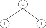
In 1969, a famous book entitled Perceptrons (Minsky & Papert, 1969) showed that it was not possible for a single-layer network, at that time called a perceptron (Figure 2.1), to represent the fundamental XOR logical function. The impact was devastating, as funding and interest in the nascent field of neural networks evaporated.
More the ten years passed until neural network research suddenly experienced a resurgence of interest. In the mid-1980s, a paper demonstrated that neural models could solve the Traveling Salesman Problem (Hopfield & Tank, 1985). Shortly thereafter, the backpropagation algorithm was created (Rummelhardt, Hinton, & Williams, 1986; Rummelhart, McClelland, & the PDP Research Group, 1987). A key demonstration showed it was possible to train a multilevel ANN to replicate an XOR truth table. In the following years, the field of neural network research and other related machine-learning fields exploded.
The importance of being able to learn and simulate the XOR truth table lies in understanding the concept of a computationally universal device. Universal Turing machines are an example of a computationally universal device (Hopcroft & Ullman, 2006) because they can, in theory, be used to simulate any other computational device.
Distinguishing ANN from perceptrons, Andreas Weigend observes:
The computational power drastically increases when an intermediate layer of nonlinear units is inserted between inputs and outputs. The example of XOR nicely emphasizes the importance of such hidden units: they re-represent the input such that the problem becomes linearly separable. Networks without hidden units cannot learn to memorize XOR, whereas networks with hidden units can implement any Boolean function. (Hertz, Krogh, & Palmer, 1991, p. 6)
In other words, the ability to simulate XOR is essential to making the argument that multilayer ANNs are universal computational devices and perceptrons without any hidden neurons are limited computational devices. It is the extra nonlinear hidden layers that give ANNs the ability to simulate other computational devices. In fact, only two layers are required to perform modeling and prediction tasks as well as symbolic learning (Lapedes & Farber, 1987a). However, clever human-aided design can create smaller networks that utilize fewer parameters, albeit with more than two hidden layers (Farber et al., 1993). Figure 2.2 shows an XOR neural network with one hidden neuron that implements a sigmoid as shown in Figure 2.3.

An Example Objective Function
The thrust::transform_reduce template makes the implementation of an objective function both straight-forward and easy. For example, an ANN least means squares objective function requires the definition of a transform operator that calculates the square of the error that the network makes on each example in the training data. A reduction operation then calculates the sum of the squared errors.
Thrust utilizes functors to perform the work of the transform and reduction operations as well as other generic methods. In C++, a functor overloads the function call operator “()” so that an object may be used in place of an ordinary function. This has several important implications:
1. Functors can be passed to generic algorithms like thrust::transform_reduce much like C-language programmers utilize pointers to functions.
2. Passing and using functors is efficient, as C++ can inline the functor code. This eliminates function call overhead and allows the compiler to perform more extensive optimizations.
3. C++ functors can maintain a persistent internal state. As you will see, this approach can be very useful when working with different device, GPU, and thread memory spaces.
Inlining of functors is essential to performance because common functors such as thrust::plus only perform tiny amounts of computation. Without the ability to inline functors, generic methods like thrust::transform_reduce would not be possible because function call overhead would consume nearly as much (or more) time than the functor itself.
The Thrust documentation speaks of kernel fusion, which combines multiple functors into a single kernel. Per our second rule of GPGPU coding, kernel fusion increases GPGPU utilization per kernel invocation, which can avoid kernel startup latencies. Just as important, many generic methods like the thrust::transform_reduce template avoid performance robbing storage of intermediate values to memory as the functor calculations are performed on the fly. The latter point meets the requirements of our third rule of GPGPU programming: focus on data reuse within the GPGPU to avoid memory bandwidth limitations. The SAXPY example in the thrust Quick Start guide provides a clear and lucid demonstration of the performance benefits of kernel fusion.
A Complete Functor for Multiple GPU Devices and the Host Processors
The following example, Example 2.2, “An XOR functor for CalcError.h,” is a complete XOR functor. The section in bold shows the simplicity to code to calculate the XOR neural network illustrated in Figure 2.2 plus error for each example in the training set.
// The CalcError functor for XOR
static const int nInput = 2;
static const int nH1 = 1;
static const int nOutput = 1;
static const int nParam =
(nOutput+nH1) // Neuron Offsets
+ (nInput*nH1) // connections from I to H1
+ (nH1*nOutput) // connections from H1 to O
+ (nInput*nOutput); // connections from I to O
static const int exLen = nInput + nOutput;
struct CalcError {
const Real* examples;
const Real* p;
const int nInput;
const int exLen;
CalcError( const Real* _examples, const Real* _p,
const int _nInput, const int _exLen)
: examples(_examples), p(_p), nInput(_nInput), exLen(_exLen) {};
__device__ __host__
Real operator()(unsigned int tid)
{
const register Real* in = &examples[tid * exLen];
register int index=0;
register Real h1 = p[index++];
register Real o = p[index++];
h1 += in[0] * p[index++];
h1 += in[1] * p[index++];
h1 = G(h1);
o += in[0] * p[index++];
o += in[1] * p[index++];
o += h1 * p[index++];
// calculate the square of the diffs
o -= in[nInput];
return o * o;
}
};
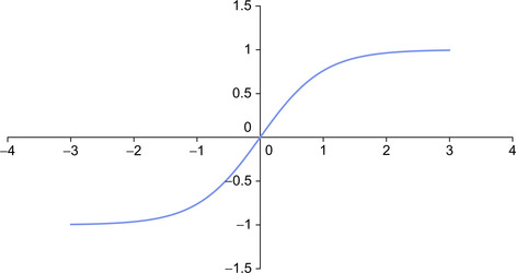
The nonlinear transfer function, G, in the previous example utilizes a hyperbolic tanh to define a sigmoid as illustrated in Figure 2.3. Other popular sigmoidal functions include the logistic function, piece-wise linear, and many others. It is easy to change the definition of G to experiment with these other functions.
It is important to note that two CUDA function qualifiers, __device__ and __host__, highlighted in the previous code snippet, specify a functor that can run on both the host processor and one or more GPU devices. This dual use of the functor makes it convenient to create hybrid CPU/GPU applications that can run on all the available computing resources in a system. It also makes performance comparisons between GPU- and host-based implementations easier.
This functor also uses persistence to encapsulate the data on the device, which ties the data to the calculation and allows work to be distributed across multiple devices and types of devices. Of course, the pointers to the vectors used by the functor should also reside on the device running the functor or undesired memory transfers will be required. CUDA 4.0 provides a unified virtual address space that allows the runtime to identify the device that contains a region of memory solely from the memory pointer. Data can then be directly transferred among devices. While the direct transfer is efficient, it still imposes PCIe bandwidth limitations.
Brief Discussion of a Complete Nelder-Mead Optimization Code
The following discussion will walk through a complete Nelder-Mead thrust API GPU example that provies single- and double-precision object instantiation, data generation, runtime configuration of the Nelder-Mead method, and a test function to verify that the network trained correctly. If desired, the code snippets in this section can be combined to create a complete xorNM.cu source file. Alternatively, a complete version of this example can be downloaded from the book's website. 6
The objective function calculates the energy. In this example, the energy is the sum of the square of the errors made by the model for a given set of parameters as shown in Equation 2.3.
(2.3)
An optimization method is utilized to fit the parameters to the data with minimal error. In this example, the Nelder-Mead method is utilized, but many other numerical techniques can be used, such as Powell's method. If the derivative of the objective function can be coded, more efficient numerical algorithms such as conjugate gradient can be used to speed the minimization process. Some of these algorithms can, in the ideal case, reduce the runtime by a factor equal to the number of parameters.
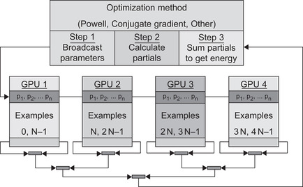
The calculation performs three steps as illustrated in Figure 2.4. For generality, multiple GPUs are shown, although the example in this chapter will work on only one GPU:
1. Broadcast the parameters from the host to the GPU(s).
2. Evaluate the objective function on the GPU. If the run utilizes multiple GPUs, then each GPU calculates a partial sum of the errors. The data set is initially partitioned across all the GPUs, where the number of examples per GPU can be used to load-balance across devices with different performance characteristics.
3. The sum (or sum of the partial sums in the multi-GPU case) is calculated via a reduce operation. In this case, thrust::transform_reduce is used to sum the errors in one operation.
The following example source code uses preprocessor conditional statements to specify the type of machine and precision of the run, which can be specified via the command line at compile time. Though conditional compilation does complicate the source code and interfere with code readability, it is a fact of life in real applications, as it facilitates code reuse and supporting multiple machine types. For this reason, conditional compilation is utilized in this book.
The following conditionals are utilized in Example 2.3, “Part 1 of xorNM.cu”:
■ USE_HOST: Selects the code that will run the objective function on the host processor. The default is to run on the GPU.
■ USE_DBL: Specifies that the compiled executable will use double-precision variables and arithmetic. The default is to use single-precision variables and arithmetic. Note that this is for convenience because C++ templates make it easy to have both single- and double-precision tests compiled by the same source code.
#include <iostream>
#include <iomanip>
#include <cmath>
#include <thrust/host_vector.h>
#include <thrust/device_vector.h>
#include <thrust/copy.h>
// define USE_HOST for a host-based version
// define USE_DBL for double precision
using namespace std;
#include "nelmin.h"
C++ polymorphism is used to make the appropriate single- and double-precision call to tanh(). See Example 2.4, “Part 2 of xorNM.cu”:
// Define the sigmoidal function
__device__ __host__
inline float G(float x) {return(tanhf(x)) ;}
__device__ __host__
inline double G(double x) {return(tanh(x));}
For convenience, a simple class, ObjFunc, was defined to combine the functor with some simple data management methods. 7 C++ templates are utilized in the example code, so the performance of the functor and overall application using single- or double-precision floating point can be evaluated. The CalcError functor defined previously is included after the comment. This use of a C-preprocessor include is not recommended for production applications. For training purposes, the functor was purposely isolated to make it easy to modify by the reader.
7C++ objects encapsulate both data and methods that operate on the data into a single convenient package.
Notice in this code section that CalcError is called directly in an OpenMP reduction loop when running on the host processor when USE_HOST is defined, which demonstrates the ability of Thrust to generate code for both GPU- and host-based functors. See Example 2.5, “Part 3 of xorNM.cu”:
// This is a convenience class to hold all the examples and
// architecture information. Most is boilerplate. CalcError
// is where all the work happens.
template<typename Real>
class ObjFunc {
private:
double objFuncCallTime;
unsigned int objFuncCallCount;
protected:
int nExamples;
#ifdef USE_HOST
thrust::host_vector<Real> h_data;
#else
thrust::device_vector<Real> d_data;
#endif
thrust::device_vector<Real> d_param;
public:
// The CalcError functor goes here
#include "CalcError.h"
// Boilerplate constructor and helper classes
ObjFunc() {nExamples = 0; objFuncCallCount=0; objFuncCallTime=0.;}
double aveObjFuncWallTime() {return(objFuncCallTime/ objFuncCallCount);}
double totalObjFuncWallTime() {return(objFuncCallTime);}
int get_nExamples() {return(nExamples);}
void setExamples(thrust::host_vector<Real>& _h_data) {
#ifdef USE_HOST
h_data = _h_data;
#else
d_data = _h_data;
#endif
nExamples = _h_data.size()/exLen;
d_param = thrust::device_vector<Real>(nParam);
}
#ifdef USE_HOST
Real objFunc(Real *p) {
if(nExamples == 0){cerr << "data not set" << endl; exit(1);}
double startTime=omp_get_wtime();
Real sum = 0.;
CalcError getError(&h_data[0], p, nInput, exLen);
#pragma omp parallel for reduction(+ : sum)
for(int i=0; i < nExamples; ++i) {
Real d = getError(i);
sum += d;
}
objFuncCallTime += (omp_get_wtime() - startTime);
objFuncCallCount++;
return(sum);
}
#else
Real objFunc(Real *p)
{
if(nExamples == 0){cerr << "data not set" <<endl; exit(1);}
double startTime=omp_get_wtime();
thrust::copy(p, p+nParam, d_param.begin());
CalcError getError(thrust::raw_pointer_cast(&d_data[0]),
thrust::raw_pointer_cast(&d_param[0]),
nInput, exLen);
Real sum = thrust::transform_reduce(
thrust::counting_iterator<unsigned int>(0),
thrust::counting_iterator<unsigned int> (nExamples),
getError,
(Real) 0.,
thrust::plus<Real>());
objFuncCallTime += (omp_get_wtime() - startTime);
objFuncCallCount++;
return(sum);
}
#endif
};
The call to the objective function must be wrapped to return the appropriate type (e.g., float or double) as seen in Example 2.6, “Part 4 of xorNM.cu.” C++ polymorphism selects the appropriate method depending on type of the parameters passed to the wrapper.
// Wrapper so the objective function can be called
// as a pointer to function for C-style libraries.
// Note: polymorphism allows easy use of
// either float or double types.
void* objFunc_object=NULL;
float func(float* param)
{
if(objFunc_object)
return ((ObjFunc<float>*) objFunc_object)->objFunc(param);
return(0.);
}
double func(double* param)
{
if(objFunc_object)
return ((ObjFunc<double>*) objFunc_object)->objFunc(param);
return(0.);
}
// get a uniform random number between −1 and 1
inline float f_rand() {
return 2.*(rand()/((float)RAND_MAX)) −1.;
}
A test function is defined to calculate the output of the function based on a set of input values. See Example 2.7, “Part 5 of xorNM.cu”:
template <typename Real, int nInput>
void testNN(const Real *p, const Real *in, Real *out)
{
int index=0;
Real h1 = p[index++];
Real o = p[index++];
h1 += in[0] * p[index++];
h1 += in[1] * p[index++];
h1 = G(h1);
o += in[0] * p[index++];
o += in[1] * p[index++];
o += h1 * p[index++];
out[0]=o;
}
For simplicity, the XOR truth table is duplicated to verify that the code works with large data sets and to provide the basis for a reasonable performance comparison between the GPGPU and host processor(s). As shown in the Example 2.8, a small amount of uniformly distributed noise with a variance of 0.01 has been added to each training example as most training data sets are noisy.
By simply defining an alternative functor and data generator, this same code framework will be adapted in Chapter 3 to solve other optimization problems. See Example 2.8, “Part 6 of xorNM.cu”:
template <typename Real>
void genData(thrust::host_vector<Real> &h_data, int nVec, Real xVar)
{
// Initialize the data via replication of the XOR truth table
Real dat[] = {
0.1, 0.1, 0.1,
0.1, 0.9, 0.9,
0.9, 0.1, 0.9,
0.9, 0.9, 0.1};
for(int i=0; i < nVec; i++)
for(int j=0; j < 12; j++) h_data.push_back(dat[j] + xVar * f_rand());
}
The testTraining() method defined in Example 2.9, “Part 7 of xorNM.cu,” sets up the Nelder-Mead optimization and calls the test function to verify the results:
template <typename Real>
void testTraining()
{
ObjFunc<Real> testObj;
const int nParam = testObj.nParam;
cout << "nParam" << nParam << endl;
// generate the test data
const int nVec=1000 * 1000 * 10;
thrust::host_vector<Real> h_data;
genData<Real>(h_data, nVec, 0.01);
testObj.setExamples(h_data);
int nExamples = testObj.get_nExamples();
cout << "GB data" << (h_data.size()*sizeof(Real)/1e9) << endl;
// set the Nelder-Mead starting conditions
int icount, ifault, numres;
vector<Real> start(nParam);
vector<Real> step(nParam,1.);
vector<Real> xmin(nParam);
srand(0);
for(int i=0; i < start.size(); i++) start[i] = 0.2 * f_rand();
Real ynewlo = testObj.objFunc(&start[0]);
Real reqmin = 1.0E-18;
int konvge = 10;
int kcount = 5000;
objFunc_object = &testObj;
double optStartTime=omp_get_wtime();
nelmin<Real> (func, nParam, &start[0], &xmin[0], &ynewlo, reqmin, &step[0], konvge, kcount, &icount, &numres, &ifault);
double optTime=omp_get_wtime()-optStartTime;
cout << endl <<"Return code IFAULT = " << ifault << endl << endl;
cout << "Estimate of minimizing value X*:" << endl << endl;
cout << "F(X*) = " << ynewlo << endl;
cout << "Number of iterations = " << icount << endl;
cout << "Number of restarts =" << numres << endl << endl;
cout << "Average wall time for ObjFunc"
<< testObj.aveObjFuncWallTime() << endl;
cout << "Total wall time in optimization method" << optTime << endl;
cout << "Percent time in objective function" <<
(100.*(testObj.totalObjFuncWallTime()/optTime)) << endl;
int index=0, nTest=4;
cout << "pred known" << endl;
thrust::host_vector<Real> h_test;
thrust::host_vector<Real> h_in(testObj.nInput);
thrust::host_vector<Real> h_out(testObj.nOutput);
genData<Real>(h_test, nTest, 0.0); // note: no variance for the test
for(int i=0; i< nTest; i++) {
h_in[0] = h_test[index++];
h_in[1] = h_test[index++];
testNN<Real,2>(&xmin[0],&h_in[0],&h_out[0]);
cout << setprecision(1) << setw(4)
<< h_out[0] << " "
<< h_test[index] << endl;
index++;
}
}
The call to main() is very simple; see Example 2.10, “Part 8 of xorNM.cu”:
int main ()
{
#ifdef USE_DBL
testTraining<double> ();
#else
testTraining<float> ();
#endif
return 0;
}
Before building, put the Nelder-Mead template from the end of this chapter into the file nelmin.h in the same directory as the xorNM.cu source code. Also ensure that CalcError.h is in the same directory.
Building all variants of xorNM.cu is straightforward. The option -use_fast_ math tells the compiler to use native GPU functions such as exp() that are fast but might not be as accurate as the software routines. Make certain that the file nelmin.h is in the same directory.
Under Linux type the code in Example 2.11, “Compiling xorNM.cu under Linux”:
# single-precision GPU test
nvcc -O3 -Xcompiler -fopenmp –use_fast_math xorNM.cu -o xorNM_GPU32
# single-precision HOST test
nvcc -D USE_HOST -O3 -Xcompiler -fopenmp xorNM.cu -o xorNM_CPU32
# double-precision HOST test
nvcc -D USE_DBL -O3 -Xcompiler -fopenmp –use_fast_math xorNM.cu -o xorNM_GPU64
# double-precision HOST test
nvcc -D USE_DBL -D USE_HOST -O3 -Xcompiler -fopenmp xorNM.cu -o xorNM_CPU64
Windows- and MacOS-based computers can utilize similar commands once nvcc is installed and the build environment is correctly configured. It is also straightforward to compile this example with Microsoft Visual Studio. Please utilize one of the many tutorials available on the Internet to import and compile CUDA applications using the Visual Studio GUI (graphical user interface).
Example 2.12, “Compiling xorNM.cu under cygwin,” is an example command to build a single-precision version of xorNM.cu for a 20-series GPU under cygwin:
nvcc -arch=sm_20 -Xcompiler "/openmp /O2" –use_fast_math xorNM.cu -o xor_gpu32.exe
Running the program shows that an ANN network is indeed trained to solve the XOR problem as illustrated by the golden test results highlighted in Example 2.13, “Example Output,” which shows that the XOR truth table is correctly predicted using the optimized parameters:
sizeof(Real) 4
Gigabytes in training vector 0.48
Return code IFAULT = 2
Estimate of minimizing value X*:
F(X*) = 4.55191e-08
Number of iterations = 5001
Number of restarts =0
Average wall time for ObjFunc 0.00583164
Total wall time in optimization method 29.5887
Percent time in objective function 98.5844
-- XOR Golden test --
pred known
0.1 0.1
0.9 0.9
0.9 0.9
0.1 0.1
Performance Results on XOR
Table 2.1 provides a sorted list of the average time to calculate the XOR objective function under a variety of precision, optimization technique, and operating system configurations. Performance was measured using a 2.53 GHz quad-core Xeon e5630 and an NVIDIA C2070 (with ECC turned off. ECC, or Error Checking and Correcting memory, means that the memory subsystem check for memory errors, which can slow performance.). The performance of an inexpensive GeForce GTX280 gaming GPU performing single-precision Nelder-Mead optimization is also shown in the table.
Performance Discussion
The average times to calculate the XOR objective function reported in Table 2.1 are based on wall clock time collected with a call to the OpenMP omp_get_wtime() method. Wall clock time is an unreliable performance measuring tool, as any other process running on the host can affect the accuracy of the timing. 8Chapter 3 discusses more advanced CUDA performance analysis tools such as the NVIDIA visual profiler for Linux and Parallel Nsight for Windows.
8It is worth noting that even tiny delays incurred by other processes briefly starting and stopping can introduce significant performance degradation in large programs running at scale, as discussed in the paper “The Case of the Missing Supercomputer Performance” (Petrini, Kerbyson, & Pakin, 2003). Cloud-based computing environments—especially those that utilize virtual machines—are especially sensitive to jitter.
All tests ran on an idle system to attain the most accurate results. Reported speedups are based on the average wall clock time consumed during the calculation of the objective function, including all host and GPU data transfers required by the objective function. OpenMP was used to multithread the host-only tests to utilize all four cores of the Xeon processor.
As Table 2.1 shows, the best performance was achieved under Linux when running a single-precision test on an NVIDIA C2070 GPGPU. Improvements in the 20-series Fermi architecture have increased double-precision performance within a factor of 2 of single-precision performance, which is significantly better than the previous generations of NVIDIA GPGPUs. Still, these older GPUs are quite powerful, as demonstrated by the 41-times-faster single-precision performance of an NVIDIA 10-series GeForce GTX280 gaming GPU over all four cores of a quad-core Xeon processor. This same midlevel gaming GPU also delivers roughly half the single-precision performance of the C2070.
The Levenberg-Marquardt results are interesting because the order of magnitude performance decrease compared to the Nelder-Mead results highlights the cost of transferring the measurement vector from the GPU to the host, as well as the performance of host-based computations needed by Levenberg-Marquardt.
This particular partitioning of a Levenberg-Marquardt optimization problem requires a large data transfer. The size of the transfer scales with the size of the data and thus introduces a scaling barrier that can make it too expensive for larger problems and multi-GPU data sets. Still, the Levenberg-Marquardt is a valid technique for GPU computing, as it can find good minima when other techniques fail. Counterintuitively, it can also run faster because it may find a minimum with just a few function calls.
In contrast, Nelder-Mead does not impose a scalability limitation, as it requires only that the GPU return a single floating-point value. Other optimization techniques such as Powell's method and conjugate gradient share this desirable characteristic.
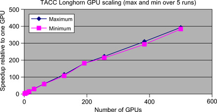
Using alternative optimization methods such as Powell's method and conjugate gradient, variants of this example code have been shown to scale to more than 500 GPGPUs on the TACC Longhorn GPGPU cluster and to tens of thousands of processors on both the TACC Ranger and Thinking Machines supercomputers (Farber, 1992; Thearling, 1995). Figure 2.5 shows the minimum and maximum speedup observed when running on 500 GPUs. It is believed that the network connecting the distributed nodes on the Longhorn GPU cluster is responsible for the variation. The benchmark was run on an idle system. More about multi-GPU applications will be discussed in Chapter 7 and the application Chapter 9, Chapter 10, Chapter 11 and Chapter 12 at the end of this book.
The advantage of the generic approach utilized by many numerical libraries is that by simply defining a new function of interest an application programmer can use the library to solve many problems. For example, the source code in this chapter will be modified in Chapter 3 to use a different functor that will perform a PCA (Principle Components Analysis). PCA along with the nonlinear variant NLPCA (Nonlinear Principle Components Analysis) has wide applicability in vision research and handwriting analysis (Hinton & Salakhutdinov, 2006) 9 as well as biological modeling (Scholz, 2011), financial modeling, Internet search, and many other commercial and academic fields.
9Available online at http://www.cs.toronto.edu/~hinton/science.pdf.
Other powerful machine-learning techniques such as Hidden Markov Models (HMM), genetic algorithms, Bayesian networks, and many others parallelize very well on GPGPU hardware. As with neural networks, each has various strengths and weaknesses. By redefining the objective function, this same example code can implement other popular techniques such as:
■ Optimization
■ Locally weighted linear regression (LWLR)
■ Naive Bayes (NB)
■ Gaussian Discriminative Analysis (GDA)
■ K-means
■ Logistic regression (LR)
■ Independent component analysis (ICA)
■ Expectation maximization (EM)
■ Support vector machine (SVM)
■ Others, such as multidimension scaling (MDS), ordinal MDS, and other variants
Summary
GPGPUs today possess a peak floating-point capability that was beyond the machines available in even the most advanced high-performance computing (HPC) centers until a Sandia National Laboratory supercomputer performed a trillion floating-point operations per second in December 1996. Many of those proposals for leading-edge research using such a teraflop supercomputer can be performed today by students anywhere in the world using a few GPGPUs in a workstation combined with a fast RAID (Redundant Array of Independent Disks) disk subsystem.
The techniques and examples discussed in this chapter can be applied to a multitude of data fitting, data analysis, dimension reduction, vision, and classification problems. Conveniently, they are able to scale from laptops to efficiently utilize the largest supercomputers in the world.
CUDA-literate programmers can bring this new world of computational power to legacy projects. Along with faster application speeds, GPGPU technology can advance the state of the art by allowing more accurate approximations and computational techniques to be utilized and ultimately to create more accurate models.
Competition is fierce in both commercial and academic circles, which is why GPU computing is making such a huge impact on both commercial products and scientific research. The competition is global; this hardware is accessible to anyone in the world who wishes to compete, as opposed to the past where competition was restricted to a relatively small community of individuals with access to big, parallel machines.
The C++ Nelder-Mead Template
#ifndef NELMIN_H
#define NELMIN_H
// Nelder-Mead Minimization Algorithm ASA047
// from the Applied Statistics Algorithms available
// in STATLIB. Adapted from the C version by J. Burkhardt
template <typename Real>
void nelmin ( Real (*fn)(Real*), int n, Real start[], Real xmin[],
Real *ynewlo, Real reqmin, Real step[], int konvge, int kcount, int *icount, int *numres, int *ifault )
{
const Real ccoeff = 0.5;
const Real ecoeff = 2.0;
const Real eps = 0.001;
const Real rcoeff = 1.0;
int ihi,ilo,jcount,l,nn;
Real del,dn,dnn;
Real rq,x,y2star,ylo,ystar,z;
//Check the input parameters.
if ( reqmin <= 0.0 ) { *ifault = 1; return; }
if ( n < 1 ) { *ifault = 1; return; }
if ( konvge < 1 ) { *ifault = 1; return; }
vector<Real> p(n*(n+1));
vector<Real> pstar(n);
vector<Real> p2star(n);
vector<Real> pbar(n);
vector<Real> y(n+1);
*icount = 0;
*numres = 0;
jcount = konvge;
dn = ( Real ) ( n );
nn = n + 1;
dnn = ( Real ) ( nn );
del = 1.0;
rq = reqmin * dn;
//Initial or restarted loop.
for ( ; ; ) {
for (int i = 0; i < n; i++ ) { p[i+n*n] = start[i]; }
y[n] = (*fn)( start );
*icount = *icount + 1;
for (int j = 0; j < n; j++ ) {
x = start[j];
start[j] = start[j] + step[j] * del;
for (int i = 0; i < n; i++ ) { p[i+j*n] = start[i]; }
y[j] = (*fn)( start );
*icount = *icount + 1;
start[j] = x;
}
//The simplex construction is complete.
//
//Find highest and lowest Y values.YNEWLO = Y(IHI) indicates
//the vertex of the simplex to be replaced.
ylo = y[0];
ilo = 0;
for (int i = 1; i < nn; i++ ) {
if ( y[i] < ylo ) { ylo = y[i]; ilo = i; }
}
//Inner loop.
for ( ; ; ) {
if ( kcount <= *icount ) {break; }
*ynewlo = y[0];
ihi = 0;
for (int i = 1; i < nn; i++ ) {
if ( *ynewlo < y[i] ) { *ynewlo = y[i]; ihi = i; }
}
//Calculate PBAR, the centroid of the simplex vertices
//excepting the vertex with Y value YNEWLO.
for (int i = 0; i < n; i++ ) {
z = 0.0;
for (int j = 0; j < nn; j++ ) { z = z + p[i+j*n]; }
z = z - p[i+ihi*n];
pbar[i] = z / dn;
}
//Reflection through the centroid.
for (int i = 0; i < n; i++ ) {
pstar[i] = pbar[i] + rcoeff * ( pbar[i] - p[i+ihi*n] );
}
ystar = (*fn)( &pstar[0] );
*icount = *icount + 1;
//Successful reflection, so extension.
if ( ystar < ylo ) {
for (int i = 0; i < n; i++ ) {
p2star[i] = pbar[i] + ecoeff * ( pstar[i] - pbar[i] );
}
y2star = (*fn)( &p2star[0] );
*icount = *icount + 1;
//Check extension.
if ( ystar < y2star ) {
for (int i = 0; i < n; i++ ) { p[i+ihi*n] = pstar[i]; }
y[ihi] = ystar;
} else { //Retain extension or contraction.
for (int i = 0; i < n; i++ ) { p[i+ihi*n] = p2star[i]; }
y[ihi] = y2star;
}
} else { //No extension.
l = 0;
for (int i = 0; i < nn; i++ ) {
if ( ystar < y[i] ) l += 1;
}
if ( 1 < l ) {
for (int i = 0; i < n; i++ ) { p[i+ihi*n] = pstar[i]; }
y[ihi] = ystar;
}
//Contraction on the Y(IHI) side of the centroid.
else if ( l == 0 ) {
for (int i = 0; i < n; i++ ) {
p2star[i] = pbar[i] + ccoeff * ( p[i+ihi*n] - pbar[i] );
}
y2star = (*fn)( &p2star[0] );
*icount = *icount + 1;
//Contract the whole simplex.
if ( y[ihi] < y2star ) {
for (int j = 0; j < nn; j++ ) {
for (int i = 0; i < n; i++ ) {
p[i+j*n] = ( p[i+j*n] + p[i+ilo*n] ) * 0.5;
xmin[i] = p[i+j*n];
}
y[j] = (*fn)( xmin );
*icount = *icount + 1;
}
ylo = y[0];
ilo = 0;
for (int i = 1; i < nn; i++ ) {
if ( y[i] < ylo ) { ylo = y[i]; ilo = i; }
}
continue;
}
//Retain contraction.
else {
for (int i = 0; i < n; i++ ) {
p[i+ihi*n] = p2star[i];
}
y[ihi] = y2star;
}
}
//Contraction on the reflection side of the centroid.
else if ( l == 1 ) {
for (int i = 0; i < n; i++ ) {
p2star[i] = pbar[i] + ccoeff * ( pstar[i] - pbar[i] );
}
y2star = (*fn)( &p2star[0] );
*icount = *icount + 1;
//
//Retain reflection?
//
if ( y2star <= ystar ) {
for (int i = 0; i < n; i++ ) { p[i+ihi*n] = p2star[i]; }
y[ihi] = y2star;
}
else {
for (int i = 0; i < n; i++ ) { p[i+ihi*n] = pstar[i]; }
y[ihi] = ystar;
}
}
}
//Check if YLO improved.
if ( y[ihi] < ylo ) { ylo = y[ihi]; ilo = ihi; }
jcount = jcount − 1;
if ( 0 < jcount ) { continue; }
//Check to see if minimum reached.
if ( *icount <= kcount ) {
jcount = konvge;
z = 0.0;
for (int i = 0; i < nn; i++ ) { z = z + y[i]; }
x = z / dnn;
z = 0.0;
for (int i = 0; i < nn; i++ ) {
z = z + pow ( y[i] − x, 2 );
}
if ( z <= rq ) {break;}
}
}
//Factorial tests to check that YNEWLO is a local minimum.
for (int i = 0; i < n; i++ ) { xmin[i] = p[i+ilo*n]; }
*ynewlo = y[ilo];
if ( kcount < *icount ) { *ifault = 2; break; }
*ifault = 0;
for (int i = 0; i < n; i++ ) {
del = step[i] * eps;
xmin[i] = xmin[i] + del;
z = (*fn)( xmin );
*icount = *icount + 1;
if ( z < *ynewlo ) { *ifault = 2; break; }
xmin[i] = xmin[i] - del - del;
z = (*fn)( xmin );
*icount = *icount + 1;
if ( z < *ynewlo ) { *ifault = 2; break; }
xmin[i] = xmin[i] + del;
}
if ( *ifault == 0 ) { break; }
//Restart the procedure.
for (int i = 0; i < n; i++ ) { start[i] = xmin[i]; }
del = eps;
*numres = *numres + 1;
}
return;
}
#endif
..................Content has been hidden....................
You can't read the all page of ebook, please click here login for view all page.