
Chapter 12. Application Focus on Live Streaming Video
CUDA lets developers write applications that can interact in real time with the user. This chapter modifies the source code from Chapter 9 to process and display live video streams. For those who do not have a webcam, live video can be imported from other machines via a TCP connection, or on-disk movie files can be used. Aside from being just plain fun, real-time video processing with CUDA opens the door to new markets in augmented reality, games, heads-up displays, face, and other generic vision recognition tasks. The example code in this chapter teaches the basics of isolating faces from background clutter, edge detection with a Sobel filter, and morphing live video streams in three dimensions. The teraflop computing capability of CUDA-enabled GPUs now gives everyone who can purchase a webcam and a gaming GPU the ability to write his or her own applications to interact with the computer visually. This includes teenagers, students, professors, and large research organizations around the world.
Keywords
Live video, Sobel edge detection, Facial segmentation, OpenGL, Primitive restart, ffmpeg, TCP, mpeg
CUDA lets developers write applications that can interact in real time with the user. This chapter modifies the source code from Chapter 9 to process and display live video streams. For those who do not have a webcam, live video can be imported from other machines via a TCP connection, or on-disk movie files can be used. Aside from being just plain fun, real-time video processing with CUDA opens the door to new markets in augmented reality, games, heads-up displays, face, and other generic vision recognition tasks. The example code in this chapter teaches the basics of isolating faces from background clutter, edge detection with a Sobel filter, and morphing live video streams in three dimensions. The teraflop computing capability of CUDA-enabled GPUs now gives everyone who can purchase a webcam and a gaming GPU the ability to write his or her own applications to interact with the computer visually. This includes teenagers, students, professors, and large research organizations around the world.
With the machine-learning techniques discussed in this book, readers have the tools required to move far beyond cookbook implementations of existing vision algorithms. It is possible to think big, as the machine-learning techniques presented in this book scale from a single GPU to the largest supercomputers in the world. However, the real value in machine learning is how it can encapsulate the information from huge (potentially terabyte) data sets into small parameterized methods that can run on the smallest cellphones and tablets.
At the end of this chapter, the reader will have a basic understanding of:
■ Managing real-time data with CUDA on Windows and UNIX computers
■ Face segmentation
■ Sobel edge detection
■ Morphing live video image data with 3D effects
■ How to create data sets from live streaming data for machine learning
Topics in Machine Vision
Machine vision is a well-established field with a large body of published material. What is new is the computational power that GPUs bring to interactive visual computing. Recall that the first teraflop supercomputer became available to the computer science elite in December 1996. Now even inexpensive NVIDIA gaming GPUs can be programmed to deliver greater performance.
Commodity webcams and freely available software revolutionize people's ability to experiment with and develop products based on live video streams. Instead of being limited to research laboratories, students can perform homework assignments using live video feeds from their webcams or based on movie files provided by their teacher. Of course, this can happen between stimulating gaming sessions using the same hardware. It is likely that these same assignments can be performed on a cell phone in the near future, given the rapid pace of development of SoC (System On a Chip) technology such as the Tegra multicore chipsets for cell phones and tablets. For example, cell phones are already being used to track faces (Tresadern, Ionita, & Cootes, 2011). 1
1A video can be seen at http://personalpages.manchester.ac.uk/staff/philip.tresadern/proj_facerec.htm.
This chapter provides a framework for study, along with several example kernels that can be used as stepping stones to visual effects, vision recognition, and augmented reality, thus bringing the world of vision research to your personal computer or laptop.
There are many resources on the Web, including a number of freely available computer vision projects, a few of which include:
■ OpenVIDIA: The OpenVIDIA package provides freely downloadable computer vision algorithms written in OpenGL, Cg, and CUDA-C. 2 The CUDA Vision workbench is a part of OpenVIDIA that provides a Windows-based application containing many common image-processing routines in a framework convenient for interactive experimentation. Additional OpenVIDIA projects include Stereo Vision, Optical Flow, and Feature Tracking algorithms.
■ GPU4Vision: This is a project founded by the Institute for Computer Graphics and Vision, Graz University of Technology. They provide publically available CUDA-based vision algorithms.
■ OpenCV: OpenCV (Open Source Computer Vision) is a library of programming functions for real-time computer vision. The software is free for both academic and commercial use. OpenCV has C++, C, Python, and other interfaces running on Windows, Linux, Android, and Mac OS X. The library boasts more than 2,500 optimized algorithms and is used around the world for applications ranging from interactive art to mine inspection, stitching maps on the Web, and advanced robotics.
3D Effects
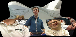
The sinusoidal demo kernel from Chapter 9 is easily modified to provide 3D effects on live data. This kernel stores the color information in the colorVBO variable. Defining the mesh to be of the same size and shape as the image allows the red, green, and blue color information in each pixel of the image to be assigned to each vertex. Any changes in the height, specified in vertexVBO, will distort the image in 3D space. Figure 12.1 shows a grayscale version of how one frame from a live stream is distorted when mapped onto the sinusoidal surface. Images produced by this example code are in full color.
Segmentation of Flesh-colored Regions
Isolating flesh-colored regions in real time from video data plays an important role in a wide range of image-processing applications including game controllers that use a video camera, face detection, face tracking, gesture analysis, sentiment analysis, and many other human computer interaction domains.
Skin color has proven to be a useful and robust cue to use as a first step in human computer processing systems (Kakumanu, Makrogiannis, & Bourbakis, 2007; Vezhnevets, Sazonov, & Andreeva, 2003). Marián Sedlácˇek provides an excellent description of the steps and assumptions used to detect human faces by first isolating skin-colored pixels (Sedláček, 2004).
The red, green, and blue (RGB) colors that represent the color of each pixel that is obtained from a webcam or other video source is not an appropriate representation to identify skin color because the RGB values vary so much when presented with varying lighting conditions and various ethnicities' skin colors. Instead, vision researchers have found that chromatic colors, normalized RGB, or “pure” colors for human skin tend to cluster tightly together regardless of skin color or luminance. Normalized pure colors—in which r, g, and b correspond to the red, green, and blue components of each pixel—are defined as “Equation 12.1: The pure red of a pixel and Equation 12.2: The pure green value of a pixel”:
(12.1)
(12.2)
The normalized blue color is redundant because PureR + PureG + PureB = 1.
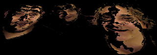
As Vezhnevets et al. note, “A remarkable property of this representation is that for matte surfaces, while ignoring ambient light, normalized RGB is invariant (under certain assumptions) to changes of surface orientation relative to the light source” (Vezhnevets, Sazonov, & Andreeva, 2003, p. 1). Though Sedlácˇek notes that the region occupied by human skin in the normalized color space is an ellipse, the example code in this chapter utilizes a rectangular region to keep the example code small. Even so, this first step in the image processing pipeline works well, as shown in Figure 12.2. Consult Sedlácˇek to see how additional steps can refine the segmentation process. 3
Edge Detection
Finding edges is a fundamental problem in image processing, as edges define object boundaries and represent important structural properties in an image. There are many ways to perform edge detection. The Sobel method, or Sobel filter, is a gradient-based method that looks for strong changes in the first derivative of an image.
The Sobel edge detector uses a pair of 3 × 3 convolution masks, one estimating the gradient in the x-direction and the other in the y-direction. This edge detector maps well to CUDA, as each thread can apply the 3 × 3 convolution masks to its pixel and adjoining pixels in the image.
Table 12.1 and Table 12.2 contain the values for the Sobel masks in each direction.
The approximate magnitude of the gradient, G, can be calculated using:
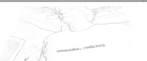
Figure 12.3 is a color inverted grayscale image created using a Sobel filter.
FFmpeg
FFmpeg is a free, open source program that can record, convert, and stream digital audio and video in various formats. It has been described as the multimedia version of a Swiss Army knife because it can convert between most common formats. The name “FFmpeg” comes from the MPEG video standards group combined with “FF” for “fast forward.” The source code can be freely downloaded from http://ffmpeg.org and compiled under most operating systems, computing platforms, and microprocessor instruction sets.
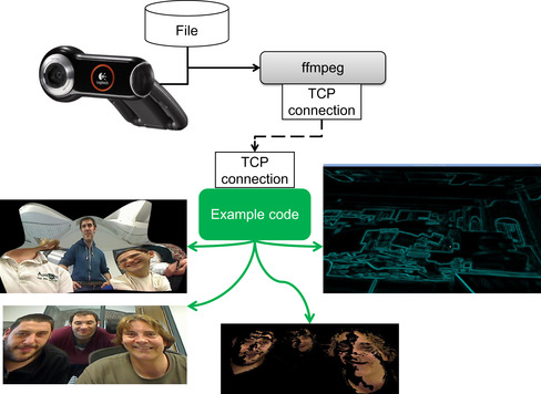
The FFmpeg command-line driven application, ffmpeg, is used in this chapter, as most readers will be able to download and use a working version for their system. As illustrated in Figure 12.4, ffmpeg is used to capture the output from a webcam or other video device and convert it to the rgb24 format, which represents each pixel in each image of the video with a separate red, green, and blue 8-bit value. The testLive example program reads the data stream from a TCP socket and writes it to a buffer on the GPU for use with CUDA. Figure 12.4 shows representative images of testLive morphing a video stream in 3D, a flat image displayed in a 3D coordinate system, segregation of faces from the background, and real-time edge detection with a Sobel filter.
The benefit of using the ffmpeg application is that no programming is required to convert the video data that can be sent to the GPU. The disadvantage is that the conversion from a compressed format to rgb24 greatly expands the amount of data sent over the TCP socket. For this reason, it is recommended that the conversion to rgb24 happen on the system containing the GPU. A more efficient implementation would use the FFmpeg libraries to directly read the compressed video stream and convert it to rgb24 within the example source code. In this way, the transport of large amounts of rgb24 data over a socket would be avoided.
Those who need to stream data from a remote webcam should:
■ Modify the example to read and perform the video conversion inside the application.
■ Use a TCP relay program to read the compressed video stream from the remote site and pass it to an instance of ffmpeg running on the system that contains the GPU. One option is socat (SOcket CAT), which is a freely downloadable general-purpose relay application that runs on most operating systems.
The following bash scripts demonstrate how to write a 640 × 480 stream of rgb24 images to port 32000 on localhost. Localhost is the name of the loopback device used by applications that need to communicate with each other on the same computer. The loopback device acts as an Ethernet interface that does not transmit information over a TCP device. Note that the ffmpeg command-line interface is evolving over time, so these scripts might need to be modified at a later date.
■ Stream from a Linux webcam (Example 12.1, “Linux Webcam Capture”):
FFMPEG=ffmpeg
DEVICE="-f video4linux2 -i /dev/video0"
PIX="-f rawvideo -pix_fmt rgb24"
SIZE="-s 640x480"
$FFMPEG -an -r 50 $SIZE $DEVICE $PIX tcp:localhost:32000
■ Stream from Windows webcam (Example 12.2, “Windows Webcam Capture”):
../ffmpeg-git-39dbe9b-win32-static/bin/ffmpeg.exe -r 25 -f vfwcap -i 0 -f rawvideo -pix_fmt rgb24 -s 640x480 tcp:localhost:32000
■ Stream from file (Example 12.3, “Stream from File”):
FFMPEG=ffmpeg
s#can be any file name or format: myfile.avi, myfile.3gp, …
FILE="myfile.mpeg"
PIX="-f rawvideo -pix_fmt rgb24"
SIZE="-s 640x480"
$FFMPEG -i $FILE $SIZE $PIX tcp:localhost:32000
Streaming from a file will run at the fastest rate that ffmpeg can convert the frames, which will likely be much faster than real-time.
TCP Server
The following code implements a simple, asynchronous TCP server that:
■ Listens on a port specified in the variable port
■ Accepts a client when one attempts to connect
■ Reads datasize bytes of data into an array when the client sends data to this server
■ Shuts down the connection when the client dies or there is a socket error and waits for another client connection
Any program can provide the rgb24 data, but it is assumed in this example that ffmpeg will supply the data.
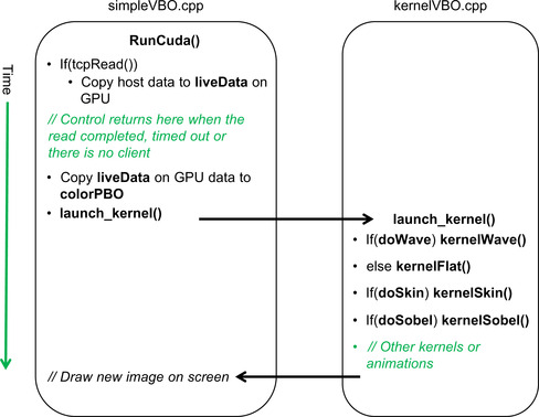
This server is asynchronous, meaning that it uses the select() call to determine whether there is a client waiting to connect or if there is data to be read. If select() times out, then control returns to the calling routine, which can perform additional work such as animating images on the screen, changing colors, or other visual effects. This process is discussed in more detail in the rest of this section and is illustrated in Figure 12.5.
The variable timeout defines how long select() will spend waiting for data to arrive on a socket. The default value is 100 microseconds, which was chosen to balance the amount of CPU time consumed by the application program versus the number of iterations of the graphic pipeline per frame of real-time data.
More information on socket programming can be found on the Internet or in excellent books such as Advanced Programming in the UNIX Environment (Stevens, 2005).
The first part of this file, tcpserver.cpp, specifies the necessary include files and variables. The initTCPserver() method binds a port that will be used to listen for client connections. It was designed to be added to the initCuda() method in simpleVBO.cu. See Example 12.4, “Part 1 of tcpserver.cpp”:
#include <sys/socket.h>
#include <netinet/in.h>
#include <stdio.h>
#include <stdlib.h>
#include <string.h>
#include <unistd.h>
#include <fcntl.h>
#include <limits.h>
int listenfd, connfd=0;
struct sockaddr_in servaddr,cliaddr;
socklen_t clilen;
struct timeval timeout = {0,100};
void initTCPserver(int port)
{
listenfd=socket(AF_INET,SOCK_STREAM,0);
bzero(&servaddr,sizeof(servaddr));
servaddr.sin_family = AF_INET;
servaddr.sin_addr.s_addr=htonl(INADDR_ANY);
servaddr.sin_port=htons(32000);
bind(listenfd,(struct sockaddr *)&servaddr,sizeof(servaddr));
}
The tcpRead() method asynchronously connects to one client at a time or performs a blocking read of datasize bytes of data when available. If no client or client data appears before select() times out, then control returns to the calling method. The debugging fprintf() statements were kept to help in understanding this code. If desired, the fprintf() statements can be uncommented to show how this code works in practice. It is recommended that the timeout should be greatly increased if the “read timeout” statement is uncommented. See Example 12.5, “Part 2 of tcpserver.cpp”:
int tcpRead(char *data, int datasize)
{
int n;
fd_set dataReady;
if(!connfd) { // there is no client: listen until timeout or accept
FD_ZERO(&dataReady);
FD_SET(listenfd,&dataReady);
if(select(listenfd+1, &dataReady, NULL,NULL, &timeout) == -1) {
fprintf(stderr,"listen select failed!
"); exit(1);
}
listen(listenfd,1); // listen for one connection at a time
clilen=sizeof(cliaddr);
if(FD_ISSET(listenfd, &dataReady)) {
fprintf(stderr,"accepting a client!
");
connfd = accept(listenfd,(struct sockaddr *)&cliaddr,&clilen);
} else {
//fprintf(stderr,"no client!
");
return(0); // no client so no work
}
}
if(!connfd) return(0);
// read the data
FD_ZERO(&dataReady);
FD_SET(connfd,&dataReady);
if(select(connfd+1, &dataReady, NULL,NULL, &timeout) == -1) {
fprintf(stderr,"data select failed!
"); exit(1);
}
if(FD_ISSET(connfd, &dataReady)) {
FD_CLR(connfd, &dataReady);
for(n=0; n < datasize;) {
int size = ((datasize-n) > SSIZE_MAX)?SSIZE_MAX:(datasize-n);
int ret = read(connfd, data+n, size);
if(ret <= 0) break; // error
n += ret;
}
if(n < datasize) {
fprintf(stderr,"Incomplete read %d bytes %d
", n, datasize);
perror("Read failure!");
close(connfd);
connfd=0;
return(0);
}
return(1);
} else {
//fprintf(stderr, "read timeout
");
}
return(0);
}
Live Stream Application
The live stream application queues CUDA kernels to perform image analysis and animated effects. Which kernels get queued depends on user input. As can be seen in Figure 12.5, new data will be transferred across the PCIe bus to the liveData buffer on the GPU only when tcpRead() returns a nonzero result, indicating a new frame of data has been read. As discussed previously, tcpRead() can return zero as a result of a timeout, in which case no new data needs to be transferred.
Because the kernel pipeline can modify the contents of colorVBO, the original video data is copied from liveData prior to the start of the pipeline. The copy from liveData to colorVBO is very fast because it moves data only within the GPU. The launch_kernel() method is then called to queue the various kernels depending on the flags set by user keystrokes in the keyboard callback.
The timeout from tcpRead() means that the launch_kernel() pipeline can be called many times between reads of new images from the live stream. Animated kernels such as kernelWave(), which produces the animated wave effect, depend on this asynchronous behavior to create their visual effects. Though not used in this example, the animTime variable can be used to control the speed and behavior of the animations.
kernelWave(): An Animated Kernel
The kernelWave() method implements the animated sinusoidal 3D surface discussed in Chapter 9. In this kernel (Example 12.6), each pixel in the image is considered as the color of a vertex in a 3D mesh. These vertex colors are held in colorVBO for the current frame in the live image. Rendering with triangles generates a smoothly colored surface, regardless of how the image is resized. For demonstration purposes, the surface can also be rendered with lines or dots depending on the user's input via the keyboard.
// live stream kernel (Rob Farber)
// Simple kernel to modify vertex positions in sine wave pattern
__global__ void kernelWave(float4* pos, uchar4 *colorPos,
unsigned int width, unsigned int height, float time)
{
unsigned int x = blockIdx.x*blockDim.x + threadIdx.x;
unsigned int y = blockIdx.y*blockDim.y + threadIdx.y;
// calculate uv coordinates
float u = x / (float) width;
float v = y / (float) height;
u = u*2.0f - 1.0f;
v = v*2.0f - 1.0f;
// calculate simple sine wave pattern
float freq = 4.0f;
float w = sinf(u*freq + time) * cosf(v*freq + time) * 0.5f;
// write output vertex
pos[y*width+x] = make_float4(u, w, v, 1.0f);
}
kernelFlat(): Render the Image on a Flat Surface
kernelFlat() simply specifies a flat surface for rendering. This allows viewing of other rendering effects without the distraction of the animated sinusoidal surface. See Example 12.7, “Part 2 of kernelVBO.cu”:
__global__ void kernelFlat(float4* pos, uchar4 *colorPos,
unsigned int width, unsigned int height)
{
unsigned int x = blockIdx.x*blockDim.x + threadIdx.x;
unsigned int y = blockIdx.y*blockDim.y + threadIdx.y;
// calculate uv coordinates
float u = x / (float) width;
float v = y / (float) height;
u = u*2.0f - 1.0f;
v = v*2.0f - 1.0f;
// write output vertex
pos[y*width+x] = make_float4(u, 1.f, v, 1.0f);
}
kernelSkin(): Keep Only Flesh-colored Regions
This kernel simply calculates the normalized red (PureR) and green (PureG) values for each pixel in the image. The original RGB colors are preserved if these values fall within the rectangle of flesh-colored tones. Otherwise, they are set to black. See Example 12.8, “Part 3 of kernelVBO.cu”
__global__ void kernelSkin(float4* pos, uchar4 *colorPos,
unsigned int width, unsigned int height,
int lowPureG, int highPureG,
int lowPureR, int highPureR)
{
unsigned int x = blockIdx.x*blockDim.x + threadIdx.x;
unsigned int y = blockIdx.y*blockDim.y + threadIdx.y;
int r = colorPos[y*width+x].x;
int g = colorPos[y*width+x].y;
int b = colorPos[y*width+x].z;
int pureR = 255*( ((float)r)/(r+g+b));
int pureG = 255*( ((float)g)/(r+g+b));
if( !( (pureG > lowPureG) && (pureG < highPureG)
&& (pureR > lowPureR) && (pureR < highPureR) ) )
colorPos[y*width+x] = make_uchar4(0,0,0,0);
}
kernelSobel(): A Simple Sobel Edge Detection Filter
The kernel in Example 12.9, “Part 4 of kernelVBO.cu,” simply applies a Sobel edge detection filter as discussed at the beginning of this chapter:
__device__ unsigned char gray(const uchar4 &pix)
{
// convert to 8-bit grayscale
return( .3f * pix.x + 0.59f * pix.y + 0.11f * pix.z);
}
__global__ void kernelSobel(float4 *pos, uchar4 *colorPos, uchar4 *newPix,
unsigned int width, unsigned int height)
{
unsigned int x = blockIdx.x*blockDim.x + threadIdx.x;
unsigned int y = blockIdx.y*blockDim.y + threadIdx.y;
const int sobelv[3][3] = { {-1,-2,-1},{0,0,0},{1,2,1}};
const int sobelh[3][3] = { {-1,0,1},{-2,0,2},{-1,0,1}};
int sumh=0, sumv=0;
if( (x > 1) && x < (width-1) && (y > 1) && y < (height-1)) {
for(int l= -1; l < 2; l++) {
for(int k= -1; k < 2; k++) {
register int g = gray(colorPos[(y+k)*width+x+l]);
sumh += sobelh[k+1][l+1] * g;
sumv += sobelv[k+1][l+1] * g;
}
}
unsigned char p = abs(sumh/8)+ abs(sumv/8);
newPix[y*width+x] = make_uchar4(0,p,p,p);
} else {
newPix[y*width+x] = make_uchar4(0,0,0,0);
}
}
The launch_kernel() Method
As illustrated in Figure 12.5, the launch_kernel() method queues kernel calls to perform the various transformation requested by the user. This method was written for clarity and not for flexibility. For example, the use of a static pointer to newPix is correct but not necessarily good coding practice. It was kept in this example code to demonstrate how the reader can allocate scratch space for his or her own methods. Once the Sobel filter completes, the scratch data is copied via a fast device-to-device transfer into the colorVBO. See Example 12.10, “Part 5 of kernelVBO.cu”:
extern int PureR[2], PureG[2], doWave, doSkin,doSobel;
// Wrapper for the __global__ call that sets up the kernel call
extern "C" void launch_kernel(float4* pos, uchar4* colorPos,
unsigned int mesh_width, unsigned int mesh_height,float time)
{
// execute the kernel
dim3 block(8, 8, 1);
dim3 grid(mesh_width / block.x, mesh_height / block.y, 1);
if(doWave)
kernelWave<<< grid, block>>>(pos, colorPos, mesh_width, mesh_height, time);
else
kernelFlat<<< grid, block>>>(pos, colorPos, mesh_width, mesh_height);
if(doSkin)
kernelSkin<<< grid, block>>>(pos, colorPos, mesh_width, mesh_height,
PureG[0], PureG[1],
PureR[0], PureR[1]);
if(doSobel) {
static uchar4 *newPix=NULL;
if(!newPix)
cudaMalloc(&newPix, sizeof(uchar4)*mesh_width*mesh_height);
kernelSobel<<< grid, block>>>(pos, colorPos, newPix,
mesh_width, mesh_height);
cudaMemcpy(colorPos, newPix, sizeof(uchar4)*mesh_width *mesh_height,
cudaMemcpyDeviceToDevice);
}
}
The simpleVBO.cpp File
Only minor changes were made to the simpleVBO.cpp file from Chapter 9, but these changes occur in several of the methods. To minimize confusion, the entire file is included at the end of this chapter with the changes highlighted.
These changes include:
■ The definition of C-preprocessor variables MESH_WIDTH and MESH_HEIGHT. These variables should be used at compile time to match the size of the mesh with the image width and height from the ffmpeg. By default, the mesh size is set to 640 × 480 pixels, which corresponds to the size specified in the ffmpeg command-line scripts at the beginning of this chapter.
■ A buffer on the GPU, liveData, is created to contain the current frame of video data. By convention, this data is not modified by the GPU between frame loads from the host.
■ The tcpRead() method is called. As can be seen in the code in the runCuda() method later in this chapter, tcpRead() has new data that needs to be transferred to the GPU when a nonzero value is returned. The runCuda() method then initializes the graphics pipeline by copying the video data to colorVBO().
The callbacksVBO.cpp File
Only minor changes were made to the callbacks.cpp file from Chapter 9; a few new variables needed to be defined. Most of the changes occur in the keyboard callback method keyboard(). Table 12.3 shows the valid keystrokes.
As mentioned in the discussion on segmentation, a rectangular region is used in the kernelSkin() method to identify human skin colors. The actual region occupied by human skin colors is an ellipse in the pure color space. A rectangular region was used because it kept the kernelSkin() method small, but with an admitted loss of fidelity. The use of a rectangle does allow the user to change the size of the rectangle with a few keystrokes to explore the effect of filtering in the color space and to see the effects of different environments and lighting conditions.
Example 12.11, “callbacksVBO.cpp,” is the modified version of the Chapter 9callbacksVBO.cpp file:
#include <GL/glew.h>
#include <cutil_inline.h>
#include <cutil_gl_inline.h>
#include <cuda_gl_interop.h>
#include <rendercheck_gl.h>
// The user must create the following routines:
void initCuda(int argc, char** argv);
void runCuda();
void renderCuda(int);
// Callback variables
extern float animTime;
extern int sleepTime, sleepInc;
int drawMode=GL_TRIANGLE_FAN; // the default draw mode
int mouse_old_x, mouse_old_y;
int mouse_buttons = 0;
float rotate_x = 0.0, rotate_y = 0.0;
float translate_z = -3.0;
// some initial values for face segmentation
int PureG[2]={62,89}, PureR[2]={112,145};
int doWave=1, doSkin=0, doSobel=0;
// GLUT callbacks display, keyboard, mouse
void display()
{
glClear(GL_COLOR_BUFFER_BIT | GL_DEPTH_BUFFER_BIT);
// set view matrix
glMatrixMode(GL_MODELVIEW);
glLoadIdentity();
glTranslatef(0.0, 0.0, translate_z);
glRotatef(rotate_x, 1.0, 0.0, 0.0);
glRotatef(rotate_y, 0.0, 1.0, 0.0);
runCuda(); // run CUDA kernel to generate vertex positions
renderCuda(drawMode); // render the data
glutSwapBuffers();
glutPostRedisplay();
// slow the rendering when the GPU is too fast.
if(sleepTime) usleep(sleepTime);
animTime += 0.01;
}
void keyboard(unsigned char key, int x, int y)
{
switch(key) {
case('q') : case(27) : // exit
exit(0);
break;
case 'd': case 'D': // Drawmode
switch(drawMode) {
case GL_POINTS: drawMode = GL_LINE_STRIP; break;
case GL_LINE_STRIP: drawMode = GL_TRIANGLE_FAN; break;
default: drawMode=GL_POINTS;
} break;
case 'S': // Slow the simulation down
sleepTime += sleepInc;
break;
case 's': // Speed the simulation up
sleepTime = (sleepTime > 0)?sleepTime -= sleepInc:0;
break;
case 'z': doWave = (doWave > 0)?0:1; break;
case 'x': doSkin = (doSkin > 0)?0:1; break;
case 'c': doSobel = (doSobel > 0)?0:1; break;
case 'R': PureR[1]++; if(PureR[1] > 255) PureR[1]=255; break;
case 'r': PureR[1]--; if(PureR[1] <= PureR[0]) PureR[1]++; break;
case 'E': PureR[0]++; if(PureR[0] >= PureR[1]) PureR[0]--; break;
case 'e': PureR[0]--; if(PureR[0] <= 0 ) PureR[0]=0; break;
case 'G': PureG[1]++; if(PureG[1] > 255) PureG[1]=255; break;
case 'g': PureG[1]--; if(PureG[1] <= PureG[0]) PureG[1]++; break;
case 'F': PureG[0]++; if(PureG[0] >= PureG[1]) PureG[0]--; break;
case 'f': PureG[0]--; if(PureG[0] <= 0 ) PureG[0]=0; break;
}
fprintf(stderr,"PureG[0] %d PureG[1] %d PureR[0] %d PureR[1] %d
",
PureG[0],PureG[1],PureR[0],PureR[1]);
glutPostRedisplay();
}
void mouse(int button, int state, int x, int y)
{
if (state == GLUT_DOWN) {
mouse_buttons |= 1<<button;
} else if (state == GLUT_UP) {
mouse_buttons = 0;
}
mouse_old_x = x;
mouse_old_y = y;
glutPostRedisplay();
}
void motion(int x, int y)
{
float dx, dy;
dx = x - mouse_old_x;
dy = y - mouse_old_y;
if (mouse_buttons & 1) {
rotate_x += dy * 0.2;
rotate_y += dx * 0.2;
} else if (mouse_buttons & 4) {
translate_z += dy * 0.01;
}
rotate_x = (rotate_x < -60.)?-60.:(rotate_x > 60.)?60:rotate_x;
rotate_y = (rotate_y < -60.)?-60.:(rotate_y > 60.)?60:rotate_y;
mouse_old_x = x;
mouse_old_y = y;
}
Building and Running the Code
The testLive application is built in the same fashion as the examples in Chapter 9. Example 12.12, “A Script to Build testLive,” is the bash build script under Linux:
#/bin/bash
DIR=livestream
SDK_PATH … /cuda/4.0
SDK_LIB0=$SDK_PATH/C/lib
SDK_LIB1= … /4.0/CUDALibraries/common/lib/linux
echo $SDK_PATH
nvcc -arch=sm_20 -O3 -L $SDK_LIB0 -L $SDK_LIB1 -I $SDK_PATH/C/common/inc simpleGLmain.cpp simpleVBO.cpp $DIR/callbacksVBO.cpp $DIR/ kernelVBO.cu tcpserver.cpp -lglut -lGLEW_x86_64 -lGLU -lcutil_x86_64 -o testLive
Running the testLive application is straightforward:
1. Start the testLive executable in one window. The visualization window will appear on your screen.
2. In a second window, run the script that will send video data to the port 32000 on localhost. Example scripts were provided at the beginning of this chapter for UNIX and for Windows and to convert a video file and send it to the testLive example.
The Future
The three examples in this chapter demonstrate real-time image processing on CUDA. However, they are but a starting point for further experimentation and research.
Machine Learning
A challenge that remains after image segmentation is identification.
Simple but valuable forms of identification can be coded as rules. For example, a game developer can look for two small flesh-colored blobs (hands) that are near a large flesh-colored blob (a face). Height differences between the hands can be used to change the angle of a simulated aircraft to make it bank and turn. Similarly, the distance between the hands can control an action such as zooming into or out of an image.
Many other tasks are not as easy to code as rules or logic in a CUDA kernel. For example, people can easily identify faces in a picture. In these cases, the machine-learning techniques presented in Chapter 2 and Chapter 3 can “learn” the algorithm for the developer using the GPU “supercomputer.” Examples abound in the literature on the use of machine learning to segment images using skin-colored pixels under general lighting conditions (Kakumanu, Makrogiannis, & Bourbakis, 2007), faces (Mitchell, 1997), and other objects. Hinton notes that machine-learning techniques like transforming autoencoders offer a better alternative than rules-based systems (Hinton, Krizhevesky, & Want, 2011). With a webcam, readers can collect their own images that can be edited and sorted into “yes” and “no” data sets to train a classifier. Both the literature and the Internet contain many detailed studies about how to use such data sets to address many problems in vision recognition.
The Connectome
The Harvard Connectome (http://cbs.fas.harvard.edu) is a project that combines GPGPU computational ability with some excellent robotic technology in an effort that will create 3D wiring diagrams of the brains of various model animals such as the cat and lab mouse. This project exemplifies early recognition of the potential inherent in GPU technology. Data from this project might prove to be the basis for seminal and disruptive scientific research. Instead of guessing, vision researchers and neurologists will finally have a Galilean first-opportunity ability to see, study, and model cortical networks using extraordinarily detailed data created by the Connectome project.
In a 2009 paper, “The Cat Is Out of the Bag: Cortical Simulations with 109 Neurons, 1013 Synapses,” researchers demonstrated that they were able to effectively model cortical networks at an unprecedented scale. In other words, these scientists feel they demonstrated sufficient computational capability to model the entire cat brain:
The simulations, which incorporate phenomenological spiking neurons, individual learning synapses, axonal delays, and dynamic synaptic channels, exceed the scale of the cat cortex, marking the dawn of a new era in the scale of cortical simulations. (Ananthanarayanan, Esser, Simon, & Modha, 2009, p. 1)
It is clear that massively parallel computational technology will open the door to detailed vision models that will allow neural research to unravel the mystery of how nature processes vision, audio, and potentially memory and thought in the brain. GPUs provide sufficient computational capability that even individuals and small research organizations have the ability to contribute to these efforts, if in no other aspect than to train the people who will make the discoveries.
Summary
CUDA is an enabling technology. As always, the power of the technology resides in the individual who uses it to solve problems. CUDA made it possible to provide working examples in the limited pages of this book to teach a range of techniques starting with the simple program in Chapter 1 that filled a vector in parallel with sequential integers, to massively parallel mappings for machine learning, and finally to the example in this chapter that performs real-time video processing. It is hoped that these examples have taught you how to use the simplicity and power of CUDA to express your thoughts concisely and clearly in software that can run on massively parallel hardware. Coupled with scalability and the teraflop floating-point capability provided by even budget GPUs, CUDA-literate programmers can leverage the power of their minds and GPU technology to do wonderful things in the world.
Listing for simpleVBO.cpp
//simpleVBO (Rob Farber)
#include <GL/glew.h>
#include <GL/gl.h>
#include <GL/glext.h>
#include <cutil_inline.h>
#include <cutil_gl_inline.h>
#include <cuda_gl_interop.h>
#include <rendercheck_gl.h>
extern float animTime;
//////////////////////////////////////////////////////////////////
// VBO specific code
#include <cutil_inline.h>
#ifndef MESH_WIDTH
#define MESH_WIDTH 640
#endif
#ifndef MESH_HEIGHT
#define MESH_HEIGHT 480
#endif
// constants
const unsigned int mesh_width = MESH_WIDTH;
const unsigned int mesh_height = MESH_HEIGHT;
const unsigned int RestartIndex = 0xffffffff;
typedef struct {
GLuint vbo;
GLuint typeSize;
struct cudaGraphicsResource *cudaResource;
} mappedBuffer_t;
extern "C"
void launch_kernel(float4* pos, uchar4* posColor,
unsigned int mesh_width, unsigned int mesh_height,
float time);
// vbo variables
mappedBuffer_t vertexVBO = {NULL, sizeof(float4), NULL};
mappedBuffer_t colorVBO = {NULL, sizeof(uchar4), NULL};
GLuint* qIndices=NULL; // index values for primitive restart
int qIndexSize=0;
uchar4 *liveData;
//////////////////////////////////////////////////////////////////
//! Create VBO
//////////////////////////////////////////////////////////////////
void createVBO(mappedBuffer_t* mbuf)
{
// create buffer object
glGenBuffers(1, &(mbuf->vbo) );
glBindBuffer(GL_ARRAY_BUFFER, mbuf->vbo);
// initialize buffer object
unsigned int size = mesh_width * mesh_height * mbuf->typeSize;
glBufferData(GL_ARRAY_BUFFER, size, 0, GL_DYNAMIC_DRAW);
glBindBuffer(GL_ARRAY_BUFFER, 0);
cudaGraphicsGLRegisterBuffer( &(mbuf->cudaResource), mbuf->vbo,
cudaGraphicsMapFlagsNone );
}
/////////////////////////////////////////////////////////////////
//! Delete VBO
/////////////////////////////////////////////////////////////////
void deleteVBO(mappedBuffer_t* mbuf)
{
glBindBuffer(1, mbuf->vbo );
glDeleteBuffers(1, &(mbuf->vbo) );
cudaGraphicsUnregisterResource( mbuf->cudaResource );
mbuf->cudaResource = NULL;
mbuf->vbo = NULL;
}
void cleanupCuda()
{
if(qIndices) free(qIndices);
deleteVBO(&vertexVBO);
deleteVBO(&colorVBO);
if(liveData) free(liveData);
}
/////////////////////////
// Add the tcp info needed for the live stream
/////////////////////////////////////////////////////////////////
#define TCP_PORT 32000
typedef struct {
unsigned char r;
unsigned char g;
unsigned char b;
} rgb24_t;
uchar4* argbData;
int argbDataSize;
extern int tcpRead(char*, int);
void initTCPserver(int);
/////////////////////////////////////////////////////////////////
//! Run the Cuda part of the computation
/////////////////////////////////////////////////////////////////
void runCuda()
{
// map OpenGL buffer object for writing from CUDA
float4 *dptr;
uchar4 *cptr;
uint *iptr;
size_t start;
cudaGraphicsMapResources( 1, &vertexVBO.cudaResource, NULL );
cudaGraphicsResourceGetMappedPointer( ( void ** )&dptr, &start,
vertexVBO.cudaResource );
cudaGraphicsMapResources( 1, &colorVBO.cudaResource, NULL );
cudaGraphicsResourceGetMappedPointer( ( void ** )&cptr, &start,
colorVBO.cudaResource );
rgb24_t data[mesh_width*mesh_height];
if(tcpRead((char*)data, mesh_width*mesh_height*sizeof(rgb24_t) )) {
// have data
#pragma omp parallel for
for(int i=0; i < mesh_width*mesh_height; i++) {
argbData[i].w=0;
argbData[i].x=data[i].r;
argbData[i].y=data[i].g;
argbData[i].z=data[i].b;
}
cudaMemcpy(liveData, argbData, argbDataSize, cudaMemcpyHostTo Device);
}
//copy the GPU-side buffer to the colorVBO
cudaMemcpy(cptr, liveData, argbDataSize, cudaMemcpyDeviceTo Device);
// execute the kernel
launch_kernel(dptr, cptr, mesh_width, mesh_height, animTime);
// unmap buffer object
cudaGraphicsUnmapResources( 1, &vertexVBO.cudaResource, NULL );
cudaGraphicsUnmapResources( 1, &colorVBO.cudaResource, NULL );
}
void initCuda(int argc, char** argv)
{
// First initialize OpenGL context, so we can properly set the GL
// for CUDA. NVIDIA notes this is necessary in order to achieve
// optimal performance with OpenGL/CUDA interop. use command-line
// specified CUDA device, otherwise use device with highest Gflops/s
if( cutCheckCmdLineFlag(argc, (const char**)argv, "device") ) {
cutilGLDeviceInit(argc, argv);
} else {
cudaGLSetGLDevice( cutGetMaxGflopsDeviceId() );
}
createVBO(&vertexVBO);
createVBO(&colorVBO);
// allocate and assign trianglefan indicies
qIndexSize = 5*(mesh_height-1)*(mesh_width-1);
qIndices = (GLuint *) malloc(qIndexSize*sizeof(GLint));
int index=0;
for(int i=1; i < mesh_height; i++) {
for(int j=1; j < mesh_width; j++) {
qIndices[index++] = (i)*mesh_width + j;
qIndices[index++] = (i)*mesh_width + j-1;
qIndices[index++] = (i-1)*mesh_width + j-1;
qIndices[index++] = (i-1)*mesh_width + j;
qIndices[index++] = RestartIndex;
}
}
cudaMalloc((void**)&liveData,sizeof(uchar4)*mesh_width*mesh_height);
// make certain the VBO gets cleaned up on program exit
atexit(cleanupCuda);
// setup TCP context for live stream
argbDataSize = sizeof(uchar4)*mesh_width*mesh_height;
cudaHostAlloc((void**) &argbData, argbDataSize, cudaHostAllocPor table );
initTCPserver(TCP_PORT);
runCuda();
}
void renderCuda(int drawMode)
{
glBindBuffer(GL_ARRAY_BUFFER, vertexVBO.vbo);
glVertexPointer(4, GL_FLOAT, 0, 0);
glEnableClientState(GL_VERTEX_ARRAY);
glBindBuffer(GL_ARRAY_BUFFER, colorVBO.vbo);
glColorPointer(4, GL_UNSIGNED_BYTE, 0, 0);
glEnableClientState(GL_COLOR_ARRAY);
switch(drawMode) {
case GL_LINE_STRIP:
for(int i=0 ; i < mesh_width*mesh_height; i+= mesh_width)
glDrawArrays(GL_LINE_STRIP, i, mesh_width);
break;
case GL_TRIANGLE_FAN: {
glPrimitiveRestartIndexNV(RestartIndex);
glEnableClientState(GL_PRIMITIVE_RESTART_NV);
glDrawElements(GL_TRIANGLE_FAN, qIndexSize, GL_UNSIGNED_INT, qIndices);
glDisableClientState(GL_PRIMITIVE_RESTART_NV);
} break;
default:
glDrawArrays(GL_POINTS, 0, mesh_width * mesh_height);
break;
}
glDisableClientState(GL_VERTEX_ARRAY);
glDisableClientState(GL_COLOR_ARRAY);
}
..................Content has been hidden....................
You can't read the all page of ebook, please click here login for view all page.