
Chapter 1. First Programs and How to Think in CUDA
The purpose of this chapter is to introduce the reader to CUDA (the parallel computing architecture developed by NVIDIA) and differentiate CUDA from programming conventional single and multicore processors. Example programs and instructions will show the reader how to compile and run programs as well as how to adapt them to their own purposes. The CUDA Thrust and runtime APIs (Application Programming Interface) will be used and discussed. Three rules of GPGPU programming will be introduced as well as Amdahl's law, Big-O notation, and the distinction between data-parallel and task-parallel programming. Some basic GPU debugging tools will be introduced, but for the most part NVIDIA has made debugging CUDA code identical to debugging any other C or C++ application. Where appropriate, references to introductory materials will be provided to help novice readers. At the end of this chapter, the reader will be able to write and debug massively parallel programs that concurrently utilize both a GPGPU and the host processor(s) within a single application that can handle a million threads of execution.
Keywords
CUDA, C++, Thrust, Runtime, API, debugging, Amdhal's law, Big-O notation, OpenMP, asynchronous, kernel, cuda-gdb, ddd
The purpose of this chapter is to introduce the reader to CUDA (the parallel computing architecture developed by NVIDIA) and differentiate CUDA from programming conventional single and multicore processors. Example programs and instructions will show the reader how to compile and run programs as well as how to adapt them to their own purposes. The CUDA Thrust and runtime APIs (Application Programming Interface) will be used and discussed. Three rules of GPGPU programming will be introduced as well as Amdahl's law, Big-O notation, and the distinction between data-parallel and task-parallel programming. Some basic GPU debugging tools will be introduced, but for the most part NVIDIA has made debugging CUDA code identical to debugging any other C or C++ application. Where appropriate, references to introductory materials will be provided to help novice readers. At the end of this chapter, the reader will be able to write and debug massively parallel programs that concurrently utilize both a GPGPU and the host processor(s) within a single application that can handle a million threads of execution.
At the end of the chapter, the reader will have a basic understanding of:
■ How to create, build, and run CUDA applications.
■ Criteria to decide which CUDA API to use.
■ Amdahl's law and how it relates to GPU computing.
■ Three rules of high-performance GPU computing.
■ Big-O notation and the impact of data transfers.
■ The difference between task-parallel and data-parallel programming.
■ Some GPU-specific capabilities of the Linux, Mac, and Windows CUDA debuggers.
■ The CUDA memory checker and how it can find out-of-bounds and misaligned memory errors.
Source Code and Wiki
Source code for all the examples in this book can be downloaded from http://booksite.mkp.com/9780123884268. A wiki (a website collaboratively developed by a community of users) is available to share information, make comments, and find teaching material; it can be reached at any of the following aliases on gpucomputing.net:
■ My name: http://gpucomputing.net/RobFarber.
■ The title of this book as one word: http://gpucomputing.net/CUDAapplicationdesignanddevelopment.
■ The name of my series: http://gpucomputing.net/supercomputingforthemasses.
Distinguishing CUDA from Conventional Programming with a Simple Example
Programming a sequential processor requires writing a program that specifies each of the tasks needed to compute some result. See Example 1.1, “seqSerial.cpp, a sequential C++ program”:
//seqSerial.cpp
#include <iostream>
#include <vector>
using namespace std;
int main()
{
const int N=50000;
// task 1: create the array
vector<int> a(N);
// task 2: fill the array
for(int i=0; i < N; i++) a[i]=i;
// task 3: calculate the sum of the array
int sumA=0;
for(int i=0; i < N; i++) sumA += a[i];
// task 4: calculate the sum of 0 .. N−1
int sumCheck=0;
for(int i=0; i < N; i++) sumCheck += i;
// task 5: check the results agree
if(sumA == sumCheck) cout << "Test Succeeded!" << endl;
else {cerr << "Test FAILED!" << endl; return(1);}
return(0);
}
Example 1.1 performs five tasks:
1. It creates an integer array.
2. A for loop fills the array a with integers from 0 to N−1.
3. The sum of the integers in the array is computed.
4. A separate for loop computes the sum of the integers by an alternate method.
5. A comparison checks that the sequential and parallel results are the same and reports the success of the test.
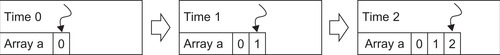
Notice that the processor runs each task consecutively one after the other. Inside of tasks 2–4, the processor iterates through the loop starting with the first index. Once all the tasks have finished, the program exits. This is an example of a single thread of execution, which is illustrated in Figure 1.1 for task 2 as a single thread fills the first three elements of array a.
This program can be compiled and executed with the following commands:
■ Linux and Cygwin users (Example 1.2, “Compiling with g++”):
g++ seqSerial.cpp –o seqSerial
./seqSerial
■ Utilizing the command-line interface for Microsoft Visual Studio users (Example 1.3, “Compiling with the Visual Studio Command-Line Interface”):
cl.exe seqSerial.cpp –o seqSerial.exe
seqSerial.exe
■ Of course, all CUDA users (Linux, Windows, MacOS, Cygwin) can utilize the NVIDIA nvcc compiler regardless of platform (Example 1.4, “Compiling with nvcc”):
nvcc seqSerial.cpp –o seqSerial
./seqSerial
In all cases, the program will print “Test succeeded!”
For comparison, let's create and run our first CUDA program seqCuda.cu, in C++. (Note: CUDA supports both C and C++ programs. For simplicity, the following example was written in C++ using the Thrust data-parallel API as will be discussed in greater depth in this chapter.) CUDA programs utilize the file extension suffix “.cu” to indicate CUDA source code. See Example 1.5, “A Massively Parallel CUDA Code Using the Thrust API”:
//seqCuda.cu
#include <iostream>
using namespace std;
#include <thrust/reduce.h>
#include <thrust/sequence.h>
#include <thrust/host_vector.h>
#include <thrust/device_vector.h>
int main()
{
const int N=50000;
// task 1: create the array
thrust::device_vector<int> a(N);
// task 2: fill the array
thrust::sequence(a.begin(), a.end(), 0);
// task 3: calculate the sum of the array
int sumA= thrust::reduce(a.begin(),a.end(), 0);
// task 4: calculate the sum of 0 .. N−1
int sumCheck=0;
for(int i=0; i < N; i++) sumCheck += i;
// task 5: check the results agree
if(sumA == sumCheck) cout << "Test Succeeded!" << endl;
else { cerr << "Test FAILED!" << endl; return(1);}
return(0);
}
Example 1.5 is compiled with the NVIDIA nvcc compiler under Windows, Linux, and MacOS. If nvcc is not available on your system, download and install the free CUDA tools, driver, and SDK (Software Development Kit) from the NVIDIA CUDA Zone (http://developer.nvidia.com). See Example 1.6, “Compiling and Running the Example”:
nvcc seqCuda.cu –o seqCuda
./seqCuda
Again, running the program will print “Test succeeded!”
Congratulations: you just created a CUDA application that uses 50,000 software threads of execution and ran it on a GPU! (The actual number of threads that run concurrently on the hardware depends on the capabilities of the GPGPU in your system.)
Aside from a few calls to the CUDA Thrust API (prefaced by thrust:: in this example), the CUDA code looks almost identical to the sequential C++ code. The highlighted lines in the example perform parallel operations.
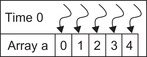
Unlike the single-threaded execution illustrated in Figure 1.1, the code in Example 1.5 utilizes many threads to perform a large number of concurrent operations as is illustrated in Figure 1.2 for task 2 when filling array a.
Choosing a CUDA API
CUDA offers several APIs to use when programming. They are from highest to lowest level:
1. The data-parallel C++ Thrust API
2. The runtime API, which can be used in either C or C++
3. The driver API, which can be used with either C or C++
Regardless of the API or mix of APIs used in an application, CUDA can be called from other high-level languages such as Python, Java, FORTRAN, and many others. The calling conventions and details necessary to correctly link vary with each language.
Which API to use depends on the amount of control the developer wishes to exert over the GPU. Higher-level APIs like the C++ Thrust API are convenient, as they do more for the programmer, but they also make some decisions on behalf of the programmer. In general, Thrust has been shown to deliver high computational performance, generality, and convenience. It also makes code development quicker and can produce easier to read source code that many will argue is more maintainable. Without modification, programs written in Thrust will most certainly maintain or show improved performance as Thrust matures in future releases. Many Thrust methods like reduction perform significant work, which gives the Thrust API developers much freedom to incorporate features in the latest hardware that can improve performance. Thrust is an example of a well-designed API that is simple yet general and that has the ability to be adapted to improve performance as the technology evolves.
A disadvantage of a high-level API like Thrust is that it can isolate the developer from the hardware and expose only a subset of the hardware capabilities. In some circumstances, the C++ interface can become too cumbersome or verbose. Scientific programmers in particular may feel that the clarity of simple loop structures can get lost in the C++ syntax.
Use a high-level interface first and choose to drop down to a lower-level API when you think the additional programming effort will deliver greater performance or to make use of some lower-level capability needed to better support your application. The CUDA runtime in particular was designed to give the developer access to all the programmable features of the GPGPU with a few simple yet elegant and powerful syntactic additions to the C-language. As a result, CUDA runtime code can sometimes be the cleanest and easiest API to read; plus, it can be extremely efficient. An important aspect of the lowest-level driver interface is that it can provide very precise control over both queuing and data transfers.
Expect code size to increase when using the lower-level interfaces, as the developer must make more API calls and/or specify more parameters for each call. In addition, the developer needs to check for runtime errors and version incompatibilities. In many cases when using low-level APIs, it is not unusual for more lines of the application code to be focused on the details of the API interface than on the actual work of the task.
Happily, modern CUDA developers are not restricted to use just a single API in an application, which was not the case prior to the CUDA 3.2 release in 2010. Modern versions of CUDA allow developers to use any of the three APIs in their applications whenever they choose. Thus, an initial code can be written in a high-level API such as Thrust and then refactored to use some special characteristic of the runtime or driver API.
Let's use this ability to mix various levels of API calls to highlight and make more explicit the parallel nature of the sequential fill task (task 2) from our previous examples. Example 1.7, “Using the CUDA Runtime to Fill an Array with Sequential Integers,” also gives us a chance to introduce the CUDA runtime API:
//seqRuntime.cu
#include <iostream>
using namespace std;
#include <thrust/reduce.h>
#include <thrust/sequence.h>
#include <thrust/host_vector.h>
#include <thrust/device_vector.h>
__global__ void fillKernel(int *a, int n)
{
int tid = blockIdx.x*blockDim.x + threadIdx.x;
if (tid < n) a[tid] = tid;
}
void fill(int* d_a, int n)
{
int nThreadsPerBlock= 512;
int nBlocks= n/nThreadsPerBlock + ((n%nThreadsPerBlock)?1:0);
fillKernel <<< nBlocks, nThreadsPerBlock >>> (d_a, n);
}
int main()
{
const int N=50000;
// task 1: create the array
thrust::device_vector<int> a(N);
// task 2: fill the array using the runtime
fill(thrust::raw_pointer_cast(&a[0]),N);
// task 3: calculate the sum of the array
int sumA= thrust::reduce(a.begin(),a.end(), 0);
// task 4: calculate the sum of 0 .. N−1
int sumCheck=0;
for(int i=0; i < N; i++) sumCheck += i;
// task 5: check the results agree
if(sumA == sumCheck) cout << "Test Succeeded!" << endl;
else { cerr << "Test FAILED!" << endl; return(1);}
return(0);
}
The modified sections of the code are in bold. To minimize changes to the structure of main(), the call to thrust::sequence() is replaced by a call to a routine fill(), which is written using the runtime API. Because array a was allocated with thrust::device_vector<>(), a call to thrust::raw_pointer_cast() is required to get the actual location of the data on the GPU. The fill() subroutine uses a C-language calling convention (e.g., passing an int* and the length of the vector) to emphasize that CUDA is accessible using both C and C++. Astute readers will note that a better C++ programming practice would be to pass a reference to the Thrust device vector for a number of reasons, including: better type checking, as fill() could mistakenly be passed a pointer to an array in host memory; the number of elements in the vector a can be safely determined with a.size() to prevent the parameter n from being incorrectly specified; and a number of other reasons.
Some Basic CUDA Concepts
Before discussing the runtime version of the fill() subroutine, it is important to understand some basic CUDA concepts:
■ CUDA-enabled GPUs are separate devices that are installed in a host computer. In most cases, GPGPUs connect to a host system via a high-speed interface like the PCIe (Peripheral Component Interconnect Express) bus.
Two to four GPGPUs can be added to most workstations or cluster nodes. How many depends on the host system capabilities such as the number of PCIe slots plus the available space, power, and cooling within the box.
Each GPGPU is a separate device that runs asynchronously to the host processor(s), which means that the host processor and all the GPGPUs can be busily performing calculations at the same time. The PCIe bus is used to transfer both data and commands between the devices. CUDA provides various data transfer mechanisms that include:
■ Explicit data transfers with cudaMemcpy() (the most common runtime data transfer method). Those who use Thrust can perform an assignment to move data among vectors (see Example 1.8, “Code Snippet Illustrating How to Move Data with Thrust”):
//Use thrust to move data from host to device
d_a = h_a;
//or from device to host
h_a = d_a;
■ Implicit transfers with mapped, pinned memory. This interface keeps a region of host memory synchronized with a region of GPU memory and does not require programmer intervention. For example, an application can load a data set on the host, map the memory to the GPU, and then use the data on the GPU as if it had been explicitly initialized with a copy operation. The use of mapped, pinned memory can increase the efficiency of a program because the transfers are asynchronous. Some low-power GPGPUs utilize host memory to save cost and power. On these devices, using mapped, pinned memory results in a zero-copy operation, as the GPU will access the data without any copy operation.
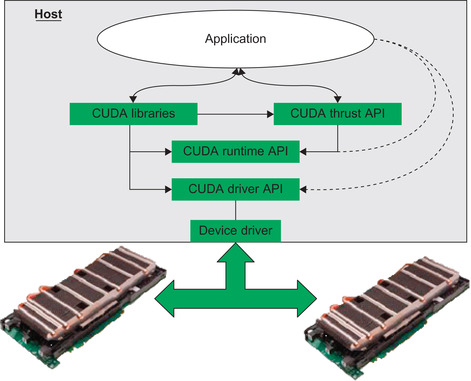
At the very lowest level, the host and GPGPU hardware interact through a software component called a device driver. The device driver manages the hardware interface so the GPU and host system can interact to communicate, calculate, and display information. It also supports many operations, including mapped memory, buffering, queuing, and synchronization. The components of the CUDA software stack are illustrated in Figure 1.3.
■ GPGPUs run in a memory space separate from the host processor. Except for a few low-end devices, all GPGPUs have their own physical memory (e.g., RAM) that have been designed to deliver significantly higher memory bandwidth than traditional host memory. Many current GPGPU memory systems deliver approximately 160–200 GB/s (gigabytes or billions of bytes per second) as compared to traditional host memory systems that can deliver 8–20 GB/s. Although CUDA 4.0 provides Unified Virtual Addressing (UVA), which joins the host and GPGPU memory into a single unified address space, do not forget that accessing memory on another device will require some transfer across the bus—even between GPGPUs. However, UVA is important because it provides software running on any device the ability to access the data on another device using just a pointer.
■ CUDA programs utilize kernels, which are subroutines callable from the host that execute on the CUDA device. It is important to note that kernels are not functions, as they cannot return a value. Most applications that perform well on GPGPUs spend most of their time in one or a few computational routines. Turning these routines into CUDA kernels is a wonderful way to accelerate the application and utilize the computational power of a GPGPU. A kernel is defined with the __global__ declaration specifier, which tells the compiler that the kernel is callable by the host processor.
■ Kernel calls are asynchronous, meaning that the host queues a kernel for execution only on the GPGPU and does not wait for it to finish but rather continues on to perform some other work. At some later time, the kernel actually runs on the GPU. Due to this asynchronous calling mechanism, CUDA kernels cannot return a function value. For efficiency, a pipeline can be created by queuing a number of kernels to keep the GPGPU busy for as long as possible. Further, some form of synchronization is required so that the host can determine when the kernel or pipeline has completed. Two commonly used synchronization mechanisms are:
■ Explicitly calling cudaThreadSynchronize(), which acts as a barrier causing the host to stop and wait for all queued kernels to complete.
■ Performing a blocking data transfer with cudaMemcpy() as cudaThreadSynchronize() is called inside cudaMemcpy().
■ The basic unit of work on the GPU is a thread. It is important to understand from a software point of view that each thread is separate from every other thread. Every thread acts as if it has its own processor with separate registers and identity (e.g., location in a computational grid) that happens to run in a shared memory environment. The hardware defines the number of threads that are able to run concurrently. The onboard GPU hardware thread scheduler decides when a group of threads can run and has the ability to switch between threads so quickly that from a software point of view, thread switching and scheduling happen for free. Some simple yet elegant additions to the C language allow threads to communicate through the CUDA shared memory spaces and via atomic memory operations.
A kernel should utilize many threads to perform the work defined in the kernel source code. This utilization is called thread-level parallelism, which is different than instruction-level parallelism, where parallelization occurs over processor instructions. Figure 1.2 illustrates the use of many threads in a parallel fill as opposed to the single-threaded fill operation illustrated in Figure 1.1.
An execution configuration defines both the number of threads that will run the kernel plus their arrangement in a 1D, 2D, or 3D computational grid. An execution configuration encloses the configuration information between triple angle brackets “<<<” and “>>>” that follow after the name of the kernel and before the parameter list enclosed between the parentheses. Aside from the execution configuration, queuing a kernel looks very similar to a subroutine call. Example 1.7 demonstrates this syntax with the call to fillKernel() in subroutine fill().
■ The largest shared region of memory on the GPU is called global memory. Measured in gigabytes of RAM, most application data resides in global memory. Global memory is subject to coalescing rules that combine multiple memory transactions into single large load or store operations that can attain the highest transfer rate to and from memory. In general, best performance occurs when memory accesses can be coalesced into 128 consecutive byte chunks. Other forms of onboard GPU programmer-accessible memory include constant, cache, shared, local, texture, and register memory, as discussed in Chapter 5.
The latency in accessing global memory can be high, up to 600 times slower than accessing a register variable. CUDA programmers should note that although the bandwidth of global memory seems high, around 160–200 GB/s, it is slow compared to the teraflop performance capability that a GPU can deliver. For this reason, data reuse within the GPU is essential to achieving high performance.
Understanding Our First Runtime Kernel
You now have the basic concepts needed to understand our first kernel.
From the programmer's point of view, execution starts on the host processor in main() of Example 1.7. The constant integer N is initialized and the Thrust method device_vector<int> is used to allocate N integers on the GPGPU device. Execution then proceeds sequentially to the fill() subroutine. A simple calculation is performed to define the number of blocks, nBlocks, based on the 512 threads per block defined by nThreadsPerBlock. The idea is to provide enough threads at a granularity of nThreadsPerBlock to dedicate one thread to each location in the integer array d_a. By convention, device variables are frequently noted by a preceding “d_” before the variable name and host variables are denoted with an “h_” before the variable name.
The CUDA kernel, fillKernel(), is then queued for execution on the GPGPU using the nBlocks and nThreadsPerBlock execution configuration. Both d_a and n are passed as parameters to the kernel. Host execution then proceeds to the return from the fill() subroutine. Note that fillKernel() must be preceded by the __global__ declaration specifier or a compilation error will occur.
At this point, two things are now happening:
1. The CUDA driver is informed that there is work for the device in a queue. Within a few microseconds (μsec or millionths of a second), the driver loads the executable on the GPGPU, defines the execution grid, passes the parameters, and—because the GPGPU does not have any other work to do—starts the kernel.
2. Meanwhile, the host processor continues its sequential execution to call thrust::reduce() to perform task 3. The host performs the work defined by the Thrust templates and queues the GPU operations. Because reduce() is a blocking operation, the host has to wait for a result from the GPGPU before it can proceed.
Once fillKernel() starts running on the GPU, each thread first calculates its particular thread ID (called tid in the code) based on the grid defined by the programmer. This example uses a simple 1D grid, so tid is calculated using three constant variables that are specific to each kernel and defined by the programmer via the execution configuration:
■ blockIdx.x: This is the index of the block that the thread happens to be part of in the grid specified by the programmer. Because this is a 1D grid, only the x component is used; the y and z components are ignored.
■ blockDim.x: The dimension or number of threads in each block.
■ threadIdx.x: The index within the block where this thread happens to be located.
The value of tid is then checked to see if it is less than n, as there might be more threads than elements in the a array. If tid contains a valid index into the a array, then the element at index tid is set to the value of tid. If not, the thread waits at the end of the kernel until all the threads complete. This example was chosen to make it easy to see how the grid locations are converted into array indices.
After all the threads finish, fillKernel() completes and returns control to the device driver so that it can start the next queued task. In this example, the GPU computes the reduction (the code of which is surprisingly complicated, as discussed in Chapter 6), and the sum is returned to the host so that the application can finish sequentially processing tasks 4 and 5.
From the preceding discussion, we can see that a CUDA kernel can be thought of in simple terms as a parallel form of the code snippet in Example 1.9, “A Sequential Illustration of a Parallel CUDA Call”:
// setup blockIdx, blockDim, and threadIdx based on the execution
// configuration
for(int i=0; i < (nBlocks * nThreadsPerBlock); i++)
fillKernel(d_a, n);
Though Thrust relies on the runtime API, careful use of C++ templates allows a C++ functor (or function object, which is a C++ object that can be called as if it were a function) to be translated into a runtime kernel. It also defines the execution configuration and creates a kernel call for the programmer. This explains why Example 1.5, which was written entirely in Thrust, does not require specification of an execution configuration or any of the other details required by the runtime API.
Three Rules of GPGPU Programming
Observation has shown that there are three general rules to creating high-performance GPGPU programs:
1. Get the data on the GPGPU and keep it there.
2. Give the GPGPU enough work to do.
3. Focus on data reuse within the GPGPU to avoid memory bandwidth limitations.
These rules make sense, given the bandwidth and latency limitations of the PCIe bus and GPGPU memory system as discussed in the following subsections.
Rule 1: Get the Data on the GPU and Keep It There
GPGPUs are separate devices that are plugged into the PCI Express bus of the host computer. The PCIe bus is very slow compared to GPGPU memory system as can be seen by the 20-times difference highlighted in Table 1.1.
Rule 2: Give the GPGPU Enough Work to Do
The adage “watch what you ask for because you might get it” applies to GPGPU performance. Because CUDA-enabled GPUs can deliver teraflop performance, they are fast enough to complete small problems faster than the host processor can start kernels. To get a sense of the numbers, let's assume this overhead is 4 μsec for a 1 teraflop GPU that takes 4 cycles to perform a floating-point operation. To keep this GPGPU busy, each kernel must perform roughly 1 million floating-point operations to avoid wasting cycles due to the kernel startup latency. If the kernel takes only 2 μsec to complete, then 50 percent of the GPU cycles will be wasted. One caveat is that Fermi GPUs can run multiple small kernels at the same time on a single GPU.
Rule 3: Focus on Data Reuse within the GPGPU to Avoid Memory Bandwidth Limitations
All high-performance CUDA applications exploit internal resources on the GPU (such as registers, shared memory, and so on, discussed in Chapter 5) to bypass global memory bottlenecks. For example, multiplying a vector by a scale factor in global memory and assigning the result to a second vector also in global memory will be slow, as shown in Example 1.10, “A Simple Vector Example”:
for(i=0; i < N; i++) c[i] = a * b[i];
Assuming the vectors require 4 bytes to store a single-precision 32-bit floating-point value in each element, then the memory subsystem of a teraflop capable computer would need to provide at least 8 terabytes per second of memory bandwidth to run at peak performance—assuming the constant scale factor gets loaded into the GPGPU cache. Roughly speaking, such bandwidth is 40 to 50 times the capability of current GPU memory subsystems and around 400 times the bandwidth of a 20-GB/s commodity processor. Double-precision vectors that require 8 bytes of storage per vector element will double the bandwidth requirement. This example should make it clear that CUDA programmers must reuse as much data as possible to achieve high performance. Please note that data reuse is also important to attaining high performance on conventional processors as well.
Big-O Considerations and Data Transfers
Big-O notation is a convenient way to describe how the size of the problem affects the consumption by an algorithm of some resource such as processor time or memory as a function of its input. In this way, computer scientists can describe the worst case (or, when specified, the average case behavior) as a function to compare algorithms regardless of architecture or clock rate. Some common growth rates are:
■ O(1): These are constant time (or space) algorithms that always consume the same resources regardless of the size of the input set. Indexing a single element in a Thrust host vector does not vary in time with the size of the data set and thus exhibits O(1) runtime growth.
■ O(N): Resource consumption with these algorithms grow linearly with the size of the input. This is a common runtime for algorithms that loop over a data set. However, the work inside the loop must require constant time.
■ O(N2): Performance is directly proportional to the square of the size of the input data set. Algorithms that use nested loops over an input data set exhibit O(N2) runtime. Deeper nested iterations commonly show greater runtime (e.g., three nested loops result in O(N3), O(N4) when four loops are nested, and so on.
There are many excellent texts on algorithm analysis that provide a more precise and comprehensive description of big-O notation. One popular text is Introduction to Algorithms (by Cormen, Leiserson, Rivest, and Stein; The MIT Press, 2009). There are also numerous resources on the Internet that discuss and teach big-O notation and algorithm analysis.
Most computationally oriented scientists and programmers are familiar with the BLAS (the Basic Linear Algebra Subprograms) library. BLAS is the de facto programming interface for basic linear algebra. NVIDIA provides a GPGPU version of BLAS with their CUBLAS library. In fact, GPGPU computing is creating a resurgence of interest in new high-performance math libraries, such as the MAGMA project at the University of Tennessee Innovative Computing Laboratory (http://icl.cs.utk.edu/magma/). MAGMA in particular utilizes both the host and a GPU device to attain high performance on matrix operations. It is available for free download.
BLAS is structured according to three different levels with increasing data and runtime requirements:
■ Level-1: Vector-vector operations that require O(N) data and O(N) work. Examples include taking the inner product of two vectors or scaling a vector by a constant multiplier.
■ Level-2: Matrix-vector operations that require O(N2) data and O(N2) work. Examples include matrix-vector multiplication or a single right-hand-side triangular solve.
■ Level-3 Matrix-vector operations that require O(N2) data and O(N3) work. Examples include dense matrix-matrix multiplication.
Table 1.2 illustrates the amount of work that is performed by each BLAS level, assuming that N floating-point values are transferred from the host to the GPU. It does not take into account the time required to transfer the data back to the GPU.
| BLAS Level | Data | Work | Work per Datum |
|---|---|---|---|
| 1 | O(N) | O(N) | O(1) |
| 2 | O(N2) | O(N2) | O(1) |
| 3 | O(N2) | O(N3) | O(N) |
Table 1.2 tells us that level-3 BLAS operations should run efficiently on graphics processors because they perform O(N) work for every floating-point value transferred to the GPU. The same work-per-datum analysis applies to non-BLAS-related computational problems as well.
To illustrate the cost of a level-1 BLAS operation, consider the overhead involved in moving data across the PCIe bus to calculate cublasScal() on the GPU and then return the vector to the host. The BLAS Sscal() method scales a vector by a constant value. CUBLAS includes a thunking interface for FORTRAN compatibility. It works by transferring data from the host to the GPU, performing the calculation, and then transferring the data back to the host from the GPU. Thunking is inefficient, as it requires moving 4N bytes of data (where N is the number of floats in the vector) twice across the PCIe bus to perform N multiplications, as shown in Example 1.10. The best possible performance would be the transfer bandwidth divided by 8 (to account for two transfers of 4N bytes of data each way), as the time to perform the multiplication would be tiny compared to the data transfers. Such an application might achieve 1 Gflop (1 billion floating-point operations per second) floating-point performance assuming an 8-GB/s transfer rate between the host and GPU. 1 Modest laptop processors and even some cell phones can exceed this calculation rate.
1Asynchronous data transfers can improve performance because the PCIe bus is full duplex, meaning that data can be transferred both to and from the host at the same time. At best, full-duplex asynchronous PCIe transfers would double the performance to two Gflop.
This analysis applies to all programs, not just level-1 and level-2 BLAS calculations. Getting good performance requires keeping as much data as possible on the GPU. After that, attaining high performance requires performing as many calculations per datum like the level-3 BLAS operations. Creating a pipeline of many lower arithmetic density computations can help, but this will only increase performance when each operation can keep the GPU busy long enough to overcome the kernel startup latency. Alternatively, it is possible to increase performance—sometime significantly—by combining multiple low-density operations like BLAS level-2 and level-2 operation into a single functor or kernel.
CUDA and Amdahl's Law
Amdahl's law is named after computer architect Gene Amdahl. It is not really a law but rather an approximation that models the ideal speedup that can happen when serial programs are modified to run in parallel. For this approximation to be valid, it is necessary for the problem size to remain the same when parallelized. In other words, assume that a serial program is modified to run in parallel. Further, assume that the amount of work performed by the program does not change significantly in the parallel version of the code, which is not always true. Obviously, those portions of the application that do not parallelize will not run any faster, and the parallel sections can run much, much faster depending on the hardware capabilities. Thus, the expected speedup of the parallel code over the serial code when using n processors is dictated by the proportion of a program that can be made parallel, P, and the portion of that cannot be parallelized, (1 − P). This relationship is shown in Equation 1.1, “Amdahl's law”.
(1.1)
Amdahl's law tells us that inventive CUDA developers have two concerns in parallelizing an application:
1. Express the parallel sections of code so that they run as fast as possible. Ideally, they should run N times faster when using N processors.
2. Utilize whatever techniques or inventiveness they have to minimize the (1 − P) serial time.
Part of the beauty of CUDA lies in the natural way it encapsulates the parallelism of a program inside computational kernels. Applications that run well on GPGPU hardware tend to have a few computationally intensive sections of the code (e.g., hotspots) that consume most of the runtime. According to Amdahl's law, these are programs with kernels that can deliver good parallel speedups (P >> 1 − P).
Observation has also shown that refactoring an application to use CUDA also tends to speed up performance on moderately parallel hardware such as multicore processors because CUDA allows developers to better see parallelism so that they can restructure the code to reduce the time spent in the serial (1 − P) sections. Of course, this assumes observation that the overhead consumed in transferring data to and from the GPGPU does not significantly affect application runtime.
Data and Task Parallelism
The examples in this chapter have thus far demonstrated data parallelism or loop-level parallelism that parallelized data operations inside the for loops. Task parallelism is another form of parallelization that reduces the (1 − P) serial time by having multiple tasks executing concurrently. CUDA naturally supports task parallelism by running concurrent tasks on the host and GPU. As will be discussed in Chapter 7, CUDA provides other ways to exploit task parallelism within a GPU or across multiple GPUs.
Even the simple GPU examples, like Example 1.5 and Example 1.7, can be modified to demonstrate task parallelism. These examples performed the following tasks:
1. Create an array.
2. Fill the array.
3. Calculate the sum of the array.
4. Calculate the sum of 0 ‥ N−1.
5. Check that the host and device results agree.
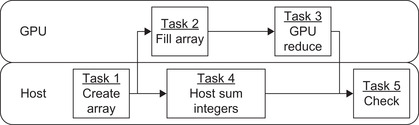
The representative timeline in Figure 1.4 shows that the previous examples do not take advantage of the asynchronous kernel execution when task 2 is queued to run on the GPU.
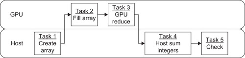
However, there is no reason why task 4 cannot be started after task 2 queues the kernel to run on the GPU. In other words, there is no dependency that forces task 4 to run after any other task, except that it must run before the check for correctness in task 5. In other words, task 5 depends on the results from task 4. Similarly, task 2 must run sometime after task 1, which allocates the array on the GPU.
Switching tasks 3 and 4 allows both the host and GPU to run in parallel, as shown in Figure 1.5, which demonstrates that it is possible to leverage CUDA asynchronous kernel execution to exploit both task and data parallelism in even this simple example. The benefit is a further reduction in application runtime.
Hybrid Execution: Using Both CPU and GPU Resources
The following example demonstrates a hybrid application that application runs simultaneously on both the CPU and GPU. Modern multicore processors are also parallel hardware that supports both data parallel and task parallel execution. OpenMP (Open Multi-Processing) is an easy way to utilize multithreaded execution on the host processor. The NVIDIA nvcc compiler supports OpenMP. Though this book is not about the OpenMP API, CUDA programmers need to know that they can exploit this host processor parallelism as well as the massive parallelism of the GPGPU. After all, the goal is to deliver the fastest application performance. It is also important to be fair when making benchmark comparisons between CPUs and GPUs by optimizing the application to achieve the highest performance on both systems to make the comparison as fair as possible.
Example 1.11, “An Asynchronous CPU/GPU Source Code” is the source code that switches the order of execution between task 3 and 4. The OpenMP parallel for loop pragma was used in task 4 to exploit data parallelism on the host processor:
//seqAsync.cu
#include <iostream>
using namespace std;
#include <thrust/reduce.h>
#include <thrust/sequence.h>
#include <thrust/host_vector.h>
#include <thrust/device_vector.h>
int main()
{
const int N=50000;
// task 1: create the array
thrust::device_vector<int> a(N);
// task 2: fill the array
thrust::sequence(a.begin(), a.end(), 0);
// task 4: calculate the sum of 0 .. N−1
int sumCheck=0;
#pragma omp parallel for reduction(+ : sumCheck)
for(int i=0; i < N; i++) sumCheck += i;
// task 3: calculate the sum of the array
int sumA= thrust::reduce(a.begin(),a.end(), 0);
// task 5: check the results agree
if(sumA == sumCheck) cout << "Test Succeeded!" << endl;
else { cerr << "Test FAILED!" << endl; return(1);}
return(0);
}
To compile with OpenMP, add “-Xcompiler -fopenmp” to the nvcc command-line argument as shown in Example 1.12 to compile Example 1.11. Because we are timing the results, the “−O3” optimization flag was also utilized.
nvcc –O3 –Xcompiler –fopenmp seqAsync.cu - seqAsync
The output from seqAsync (Example 1.13, “Results Showing a Successful Test”) shows that the sum is correctly calculated as it passes the golden test:
$ ./a.out
Test Succeeded!
Regression Testing and Accuracy
As always in programming, the most important metric for success is that the application produces the correct output. Regression testing is a critical part of this evaluation process that is unfortunately left out of most computer science books. Regression tests act as sanity checks that allow the programmer to use the computer to detect if some error has been introduced into the code. The computer is impartial and does not get tired. For these reasons, small amounts of code should be written and tested to ensure everything is in a known working state. Additional code can then be added along with more regression tests. This greatly simplifies debugging efforts as the errors generally occur in the smaller amounts of new code. The alternative is to write a large amount of code and hope that it will work. If there is an error, it is challenging to trace through many lines of code to find one or more problems. Sometimes you can get lucky with the latter approach. If you try it, track your time to see if there really was a savings over taking the time to use regression testing and incremental development.
The examples in this chapter use a simple form of regression test, sometimes called a golden test or smoke test, which utilizes an alternative method to double-check the parallel calculation of the sum of the integers. Such simple tests work well for exact calculations, but become more challenging to interpret when using floating-point arithmetic due to the numerical errors introduced into a calculation when using floating-point. As GPGPU technology can perform several trillion floating-point operations per second, numerical errors can build up quickly. Still, using a computer to double-check the results beats staring at endless lines of numbers. For complex programs and algorithms, the regression test suite can take as much time to plan, be as complex to implement, and require more lines of code than the application code itself!
While hard to justify to management, professors or to you (especially when working against a tight deadline), consider the cost of delivering an application that does not perform correctly. For example, the second startup I co-founded delivered an artificial learning system that facilitated the search for candidate drug leads using some of the technology discussed later in this book. The most difficult question our startup team had to answer was posed by the research executive committee of a major investor. That question was “how do we know that what you are doing on the computer reflects what really happens in the test tube?” The implied question was, “how do we know that you aren't playing some expensive computer game with our money?” The solution was to perform a double-blind test showing that our technology could predict the chemical activity of relevant compounds in real-world experiments using only on a very small set of measurements and no knowledge of the correct result. In other words, our team utilized a form of sanity checking to demonstrate the efficacy of our model and software. Without such a reality check, it likely that the company would not have received funding.
Silent Errors
A challenge with regression testing is that some errors can still silently pass through the test suite and make it to the application that the end-user sees. For example, Andy Regan at ICHEC (the Irish Center for High-End Computing) pointed out that increasing the value of N in the examples in this chapter can cause the sum to become so large that it cannot be contained in an integer. Some systems might catch the error and some systems will miss the error.
Given that GPUs can perform a trillion arithmetic operations per second, it is important that CUDA programmers understand how quickly numerical errors can accumulate or computed values overflow their capacity. A quick introduction to this topic is my Scientific Computing article “Numerical Precision: How Much Is Enough?” (Farber, 2009), which is freely available on the Internet.
Thrust provides the ability to perform a reduction where smaller data types are converted into a larger data type, seqBig.cu, demonstrates how to use a 64-bit unsigned integer to sum all the 32-bit integers in the vector. The actual values are printed at the end of the test. See Example 1.14, “A Thrust Program that Performs a Dual-Precision Reduction”:
//seqBig.cu
#include <iostream>
using namespace std;
#include <thrust/reduce.h>
#include <thrust/sequence.h>
#include <thrust/host_vector.h>
#include <thrust/device_vector.h>
int main()
{
const int N=1000000;
// task 1: create the array
thrust::device_vector<int> a(N);
// task 2: fill the array
thrust::sequence(a.begin(), a.end(), 0);
// task 3: calculate the sum of the array
unsigned long long sumA= thrust::reduce(a.begin(),a.end(),
(unsigned long long) 0, thrust::plus<unsigned long long>() );
// task 4: calculate the sum of 0 .. N−1
unsigned long long sumCheck=0;
for(int i=0; i < N; i++) sumCheck += i;
cerr << "host" << sumCheck << endl;
cerr << "device " << sumA << endl;
// task 5: check the results agree
if(sumA == sumCheck) cout << "Test Succeeded!" << endl;
else { cerr << "Test FAILED!" << endl; return(1);}
return(0);
}
The nvcc compiler has the ability to compile and run an application from a single command-line invocation. Example 1.15, “Results Showing a Successful Test” shows the nvcc command line and the successful run of the seqBig.cu application:
$ nvcc seqBig.cu -run
host499999500000
device 499999500000
Test Succeeded!
Can you find any other silent errors that might occur as the size of N increases in these examples? (Hint: what limitations does tid have in the runtime example?)
Introduction to Debugging
Debugging programs is a fact of life—especially when learning a new language. With a few simple additions, CUDA enables GPGPU computing, but simplicity of expression does not preclude programming errors. As when developing applications for any computer, finding bugs can be complicated.
Following the same economy of change used to adapt C and C++, NVIDIA has extended several popular debugging tools to support GPU computing. These are tools that most Windows and UNIX developers are already proficient and comfortable using such as gdb, ddd, and Visual Studio. Those familiar with building, debugging, and profiling software under Windows, Mac, and UNIX should find the transition to CUDA straightforward. For the most part, NVIDIA has made debugging CUDA code identical to debugging any other C or C++ application. All CUDA tools are freely available on the NVIDIA website, including the professional edition of Parallel Nsight for Microsoft Visual Studio.
UNIX Debugging
NVIDIA's cuda-gdb Debugger
To use the CUDA debugger, cuda-gdb, the source code must be compiled with the -g -G flags. The -g flag specifies that the host-side code is to be compiled for debugging. The -G flag specifies that the GPU side code is to be compiled for debugging (see Example 1.16, “nvcc Command to Compile for cuda-gdb”):
nvcc −g −G seqRuntime.cu −o seqRuntime
Following is a list of some common commands, including the single-letter abbreviation and a brief description:
■ breakpoint (b): set a breakpoint to stop the program execution at selected locations in the code. The argument can either be a method name or line number.
■ run (r): run the application within the debugger.
■ next (n): move to the next line of code.
■ continue (c): continue to the next breakpoint or until the program completes.
■ backtrace (bt): shows contents of the stack including calling methods.
■ thread: lists the current CPU thread.
■ cuda thread: lists the current active GPU threads (if any).
■ cuda kernel: lists the currently active GPU kernels and also allows switching “focus” to a given GPU thread.
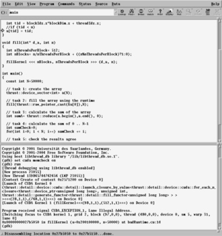
Use cuda-gdb to start the debugger, as shown in Example 1.17, “cuda-gdb Startup”:
$ cuda-gdb seqRuntime
NVIDIA (R) CUDA Debugger
4.0 release
Portions Copyright (C) 2007-2011 NVIDIA Corporation
GNU gdb 6.6
Copyright (C) 2006 Free Software Foundation, Inc.
GDB is free software, covered by the GNU General Public License, and you are welcome to change it and/or distribute copies of it under certain conditions.
Type "show copying" to see the conditions.
There is absolutely no warranty for GDB. Type "show warranty" for details.
This GDB was configured as "x86_64-unknown-linux-gnu"…
Using host libthread_db library "/lib/libthread_db.so.1".
Use the “l” command to show the source for fill, as shown in Example 1.18, “cuda-gdb List Source Code”:
(cuda-gdb) l fill
11int tid = blockIdx.x*blockDim.x + threadIdx.x;
12if (tid < n) a[tid] = tid;
13}
14
15void fill(int* d_a, int n)
16{
17int nThreadsPerBlock= 512;
18int nBlocks= n/nThreadsPerBlock + ((n%nThreadsPerBlock)?1:0);
19
20fillKernel <<< nBlocks, nThreadsPerBlock >>> (d_a, n);
Set a breakpoint at line 12 and run the program. We see that a thrust kernel runs and then the breakpoint is hit in fillkernel(), as shown in Example 1.19, “cuda-gdb Set a Breakpoint”:
(cuda-gdb) b 12
Breakpoint 1 at 0x401e30: file seqRuntime.cu, line 12.
(cuda-gdb) r
Starting program: /home/rmfarber/foo/ex1-3
[Thread debugging using libthread_db enabled]
[New process 3107]
[New Thread 139660862195488 (LWP 3107)]
[Context Create of context 0x1ed03a0 on Device 0]
Breakpoint 1 at 0x20848a8: file seqRuntime.cu, line 12.
[Launch of CUDA Kernel 0 (thrust::detail::device::cuda::detail::launch_closure_by_value<thrust::detail::device::cuda::for_each_n_closure<thrust::device_ptr<unsigned long long>, unsigned int, thrust::detail::generate_functor<thrust::detail::fill_functor<unsigned long long> > > ><<<(28,1,1),(768,1,1)>>>) on Device 0]
[Launch of CUDA Kernel 1 (fillKernel<<<(1954,1,1),(512,1,1)>>>) on Device 0]
[Switching focus to CUDA kernel 1, grid 2, block (0,0,0), thread (0,0,0), device 0, sm 0, warp 0, lane 0]
Breakpoint 1, fillKernel<<<(1954,1,1),(512,1,1)>>> (a=0x200100000, n=50000)
at seqRuntime.cu:12
12if (tid < n) a[tid] = tid;
Print the value of the thread Id, tid, as in Example 1.20, “cuda-gdb Print a Variable”:
(cuda-gdb) p tid
$1 = 0
Switch to thread 403 and print the value of tid again. The value of tid is correct, as shown in Example 1.21, “cuda-gdb Change Thread and Print a Variable”:
(cuda-gdb) cuda thread(403)
[Switching focus to CUDA kernel 1, grid 2, block (0,0,0), thread (403,0,0), device 0, sm 0, warp 12, lane 19]
12if (tid < n) a[tid] = tid;
(cuda-gdb) p tid
$2 = 403
Exit cuda-gdb (Example 1.22, “cuda-gdb Exit”):
(cuda-gdb) quit
The program is running.Exit anyway? (y or n) y
This demonstrated only a minimal set of cuda-gdb capabilities. Much more information can be found in the manual “CUDA-GDB NVIDIA CUDA Debugger for Linux and Mac,” which is updated and provided with each release of the CUDA tools. Parts 14 and 17 of my Doctor Dobb's Journal tutorials discuss cuda-gdb techniques and capabilities in much greater depth. Also, any good gdb or ddd tutorial will also help novice readers learn the details of cuda-gdb.
The CUDA Memory Checker
Unfortunately, it is very easy to make a mistake when specifying the size of a dynamically allocated region of memory. In many cases, such errors are difficult to find. Programming with many threads compounds the problem because an error in thread usage can cause an out-of-bounds memory access. For example, neglecting to check whether tid is less than the size of the vector in the fill routine will cause an out-of-bounds memory access. This is a subtle bug because the number of threads utilized is specified in a different program location in the execution configuration. See Example 1.23, “Modified Kernel to Cause an Out-of-Bounds Error”:
__global__ void fillKernel(int *a, int n)
{
int tid = blockIdx.x*blockDim.x + threadIdx.x;
// if(tid < n) // Removing this comparision introduces an out-of-bounds error
a[tid] = tid;
}
The CUDA tool suite provides a standalone memory check utility called cuda-memcheck. As seen in Example 1.24, “Example Showing the Program Can Run with an Out-of-Bounds Error,” the program appears to run correctly:
$ cuda-memcheck badRuntime
Test Succeeded!
However cuda-memcheck correctly flags that there is an out-of-bounds error, as shown in Example 1.25, “Out-of-Bounds Error Reported by cuda-memcheck”:
$ cuda-memcheck badRuntime
========= CUDA-MEMCHECK
Test Succeeded!
========= Invalid __global__ write of size 4
=========at 0x000000e0 in badRuntime.cu:14:fillKernel
=========by thread (336,0,0) in block (97,0,0)
=========Address 0x200130d40 is out of bounds
=========
========= ERROR SUMMARY: 1 error
Notice that no special compilation flags were required to use cuda-memcheck.
Use cuda-gdb with the UNIX ddd Interface
The GNU ddd (Data Display Debugger) provides a visual interface for cuda-gdb (or gdb). Many people prefer a visual debugger to a plain-text interface. To use cuda-gdb, ddd must be told to use a different debugger with the “-debugger” command-line flag as shown in Example 1.26, “Command to Start ddd with cuda-gdb”:
ddd –debugger cuda-gdb badRuntime
Break points can be set visually, and all cuda-gdb commands can be manually entered. The following screenshot shows how to find an out-of-bounds error by first specifying set cuda memcheck on. As will be demonstrated in Chapter 3, ddd also provides a useful machine instruction window to examine and step through the actual instructions the GPU is using. See Example 1.27, “Using cuda-gdb Inside ddd to Find the Out-of-Bounds Error”:
 |
Windows Debugging with Parallel Nsight
Parallel Nsight also provides a debugging experience familiar to Microsoft Visual Studio users yet includes powerful GPU features like thread-level debugging and the CUDA memory checker. It installs as a plug-in within Microsoft Visual Studio. Parallel insight also provides a number of features:
■ Integrated into Visual Studio 2008 SP1 or Visual Studio 2010.
■ CUDA C/C++ debugging.
■ DirectX 10/11 shader debugging.
■ DirectX 10/11 frame debugging.
■ DirectX 10/11 frame profiling.
■ CUDA kernel trace/profiling.
■ OpenCL kernel trace/profiling.
■ DirectX 10/11 API & HW trace.
■ Data breakpoints for CUDA C/C++ code.
■ Analyzer/system trace.
■ Tesla Compute Cluster (TCC) support.
Parallel Nsight allows both debugging and analysis on the machine as well as on remote machines that can be located at a customer's site. The capabilities of Parallel Nsight vary with the hardware configuration seen in Table 1.3.
Figure 1.6 shows Parallel Nsight stopped at a breakpoint on the GPU when running the fillkernel() kernel in seqRuntime.cu. The locals window shows the values of various variables on the GPU.
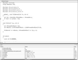
A screenshot does not convey the interactive nature of Parallel Nsight, as many of the fields on the screen are interactive and can be clicked to gain more information. Visual Studio users should find the Parallel Nsight comfortable, as it reflects and utilized the look and feel of other aspects of Visual Studio. Parallel Nsight is an extensive package that is growing and maturing quickly. The most current information, including videos and the user forums, can be found on the Parallel Nsight web portal at http://www.nvidia.com/ParallelNsight as well as the help section in Visual Studio.
Summary
This chapter covered a number of important applied topics such as how to write, compile, and run CUDA applications on the GPGPU using both the runtime and Thrust APIs. With the tools and syntax discussed in this chapter, it is possible to write and experiment with CUDA using the basics of the Thrust and runtime APIs. Audacious readers may even attempt to write real applications, which is encouraged, as they can be refactored based on the contents of later chapters and feedback from the performance profiling tools. Remember, the goal is to become a proficient CUDA programmer and writing code is the fastest path to that goal. Just keep the three basic rules of GPGPU programming in mind:
1. Get the data on the GPGPU and keep it there.
2. Give the GPGPU enough work to do.
3. Focus on data reuse within the GPGPU to avoid memory bandwidth limitations.
Understanding basic computer science concepts is also essential to achieving high performance and improving yourself as a computer scientist. Keep Amdahl's law in mind to minimize serial bottlenecks as well as exploiting both task and data parallelism. Always try to understand the big-O implications of the algorithms that you use and seek out alternative algorithms that exhibit better scaling behavior. Always attempt to combine operations to achieve the highest computational density on the GPU while minimizing slow PCIe bus transfers.
..................Content has been hidden....................
You can't read the all page of ebook, please click here login for view all page.