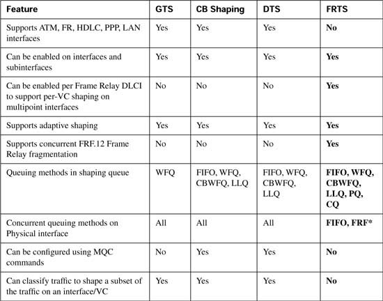
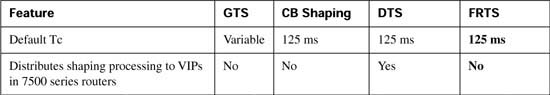
Table B-30 lists the comparison features for the shaping tools, with DTS highlighted.
Frame Relay traffic shaping (FRTS) differs from the other three shaping tools in several significant ways. The most obvious difference is the most important—FRTS applies to Frame Relay only. But the basic shaping function is the same, with the same parameters—a shaped rate, which is often set to CIR; a Tc interval, which defaults to 125 ms; and the Bc value is either set, or calculated based on the Tc = Bc/CIR formula.
The first big difference between FRTS and the other shapers has to do with queuing tool support. FRTS does not allow any IOS queuing tool to be used on the physical interface when FRTS is configured for VCs on the interface. Even if a queuing tool has already been configured, IOS removes the configuration from the physical interface when FRTS is enabled. FRTS does supply the largest list of options for queuing tools for the shaping queue: FIFO, PQ, CQ, CBWFQ, LLQ, and WFQ are all available.
For you exam takers, be aware that at the time this book went to press the Cisco QoS course book incorrectly claims that FRTS supports WFQ on the physical interface; the DQOS course book does not say anything about queuing on the physical interface with FRTS.
The next important difference is that FRTS supports concurrent Frame Relay fragmentation (FRF) using Frame Relay Forum Implementation Agreement 12, also known as FRF.12. With FRF.12, large packets are fragmented, with “large” being defined with configuration commands. Small packets are interleaved, so that a small packet does not have to wait on the long serialization delay associated with the longer original packets. Interestingly, to perform the interleaving feature, FRF uses two queues on the physical interface, with one of the queues holding small, unfragmented packets, and the other holding the fragments of large packets. The queue holding the unfragmented packets is treated like a low-latency queue, always being serviced first. Therefore, although FRTS does not allow any queuing tools on the physical interface, FRF.12 supplies the added benefit of at least a two-queue system, called dual-FIFO, to the physical interface.
FRTS, unlike the other shaping tools, cannot shape a subset of the traffic on an interface. Each of the other three shapers can be configured on one subinterface, and not the other, essentially enabling shaping on only some of the traffic leaving an interface. The other three shapers can also configure classification parameters, and shape only part of the traffic on a subinterface. Unlike the other shapers, when FRTS is enabled on the physical interface, all traffic on the interface is shaped in some way. In fact, with FRTS enabled, each VC is shaped separately. However, you cannot enable FRTS for only a subset of the VCs on an interface, nor for a subset of the traffic exiting a single VC.
FRTS shapes all VCs on an interface after it has been enabled on that interface. To enable FRTS, add the frame-relay traffic-shape command under the physical interface. If you add no other configuration commands, FRTS uses default settings and shapes each individual VC. If you include additional configuration per VC, FRTS uses those parameters rather than the defaults. In any case, FRTS always shapes each VC separately after it has been enabled on the physical interface.
Unlike the other three shapers, FRTS can dynamically learn the CIR, Bc, and Be values configured per VC at the Frame Relay switch and use those settings for shaping. Cisco’s WAN switching products (from the Stratacom acquisition in the mid-1990s) use an Enhanced LMI (ELMI) feature, which IOS understands. Using ELMI, the switch just announces the CIR, Bc, and Be for each VC to the router. So, if you want to use FRTS only to shape to CIR, and the Frame Relay network uses Cisco switches, you can just enable FRTS and ELMI on the interface, and the rest (Bc, CIR, and so on) will be learned dynamically for each VC.
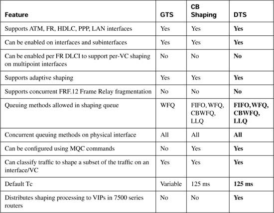
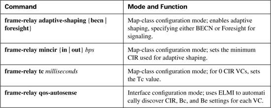
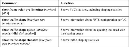
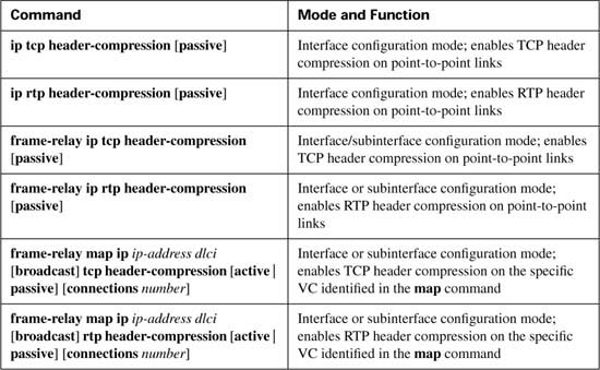
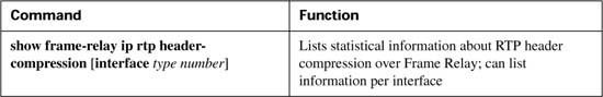
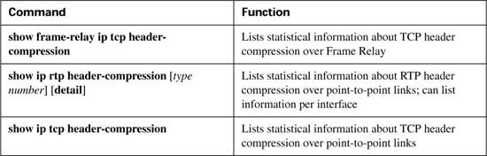
Finally, the biggest difference relates to FRTS configuration. The commands used differ totally from the other three tools. Tables B-31 and B-32 list the configuration and show commands pertinent to FRTS, respectively.
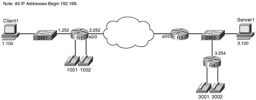
For the sake of comparison, the first FRTS example follows the same requirements as the first GTS and CB shaping examples. The configuration shows R3, with a 128-kbps access rate, and a 64-kbps Frame Relay VC connecting to R1. The criteria for the configuration is as follows:
![]() Shape all traffic at a 64-kbps rate.
Shape all traffic at a 64-kbps rate.
![]() Use the default setting for Tc.
Use the default setting for Tc.
![]() Do not use a Be.
Do not use a Be.
![]() Enable the configuration on the subinterface.
Enable the configuration on the subinterface.
![]() Do not specify a particular queuing method for the shaping queue.
Do not specify a particular queuing method for the shaping queue.
In each example, the client downloads one web page, which has two frames inside the page. The web page uses two separate TCP connections to download two separate large JPG files. The PC also downloads a file using FTP get. In addition, a VoIP call is placed between extension 302 and 102. Example B-27 shows the configuration and some sample show commands.

FRTS configuration typically involves three separate steps, although only the first step is actually required.
Step 1 FRTS must be enabled on the physical interface with the frame-relay traffic-shape interface subcommand. This is the only required step.
Step 2 The shaping parameters—the shaping rate, Bc, and Be—need to be configured inside a FRTS map-class command.
Step 3 The shaping parameters defined in the map-class should be enabled on the interface, subinterface, or DLCI using the frame-relay class class-name command.
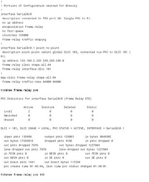
All three steps were used in Example B-27. The frame-relay traffic-shape interface subcommand, under serial 0/0, enables FRTS. Next, the frame-relay class shape-all-64 subinterface subcommand tells the router to use the shaping parameters in the map-class called shape-all-64. Finally, the map-class frame-relay shape-all-64 command creates a map class, with the frame-relay traffic-rate 64000 64000 command specifying the shaping rate of 64,000 bps. From the first 64000 parameter, FRTS calculates the Bc and Tc values. The second 64000 in the command sets the excess information rate (EIR), from which the Be is calculated; to have a burst greater than zero, the excess rate must be larger than the shaping rate.
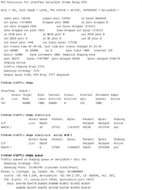
The show frame-relay pvc command, which follows the configuration in the example, lists statistics about each Frame Relay permanent virtual circuit (PVC). However, the show frame- relay pvc 101 command, with a specific VC listed, gives some basic information about FRTS operation on the VC. In this case, the output shows that shaping is active, which means that FRTS was actively shaping packets when this command was issued. (As with other shapers, FRTS shaping is active when packets are in the shaping queues, or as soon as a packet exceeds the traffic contract so that it should be placed in the queues.) The command also lists that the default queuing type of FIFO is used, along with some statistics about the number of packets tail dropped from the shaping queue.
The same show traffic-shape commands used with GTS also provide useful information for FRTS. The show traffic-shape command output shown in Example B-27 lists the basic shaping settings. Remember, the frame-relay traffic-rate 64000 64000 command did not explicitly set Bc, Be, or Tc, but Bc and Be are shown in the show traffic-shape command output. The logic to derive the values works like this, with CIR representing the configured shaping rate:
![]() Tc defaults to 125 ms
Tc defaults to 125 ms
![]() Bc = Tc * CIR (in this example, Bc = .125 * 64000 = 8000)
Bc = Tc * CIR (in this example, Bc = .125 * 64000 = 8000)
![]() Be = Tc * (EIR – CIR)
Be = Tc * (EIR – CIR)
In this example, the shaping parameters are set as follows:
![]() Tc defaults to 125 ms
Tc defaults to 125 ms
![]() Bc = .125 * 64000 = 8000
Bc = .125 * 64000 = 8000
![]() Be = .125 * (64000 – 64000) = 0
Be = .125 * (64000 – 64000) = 0
For each Tc of 125 ms, FRTS allows 8000 bits, so the overall rate becomes 64,000 bps.
Those of you who are thoroughly reading the command output may have noticed that the show traffic-shape command actually lists Bc as 64,000, not the 8000 bits suggested previously. Interestingly, when using the frame-relay traffic-rate command, the show traffic-shape “Sustained Bits/interval” heading lists the bits per second. Internally, a 125-ms Tc value is really used, and a Bc of 8000 is really used—but the output of the command lists the number of bits that can be sent in a full second. The value of 1000 bytes under the heading “Increment (Bytes)” accurately lists the real Bc value used. (I did not believe it either; check out www.cisco.com/univercd/cc/td/doc/product/software/ios122/122cgcr/fwan_r/frcmds/wrffr3.htm#xtocid24, and look for the frame-relay traffic-rate command, for some confirming comments.)
The show traffic-shape statistics and the show traffic-shape queue commands list the same basic information for FRTS as they did for GTS. One piece of terminology not seen with GTS, however, is that the default queuing type of FRTS shaping tools is called “FCFS” in the show command output. FCFS stands for first-come, first-served, which is just another term for FIFO.
You can configure basic FRTS shaping parameters in two ways. The first example, Example B-27, used the traffic-shape rate command. Alternatively, you can use the frame-relay cir, frame- relay Bc, and frame-relay Be commands to set FRTS shaping parameters inside an FRTS map class. In fact, if you want to manipulate Tc down to a smaller value, which you typically should do to support voice and video traffic, you must use these alternative commands. Remember, Tc = Bc/shaped rate, or Tc = Bc/CIR if you are shaping at the CIR. Example B-28 lists two examples that use these additional FRTS commands, with show commands listing the changed Tc and Bc values. The commands are applied to R3, the same router as in Example B-27.
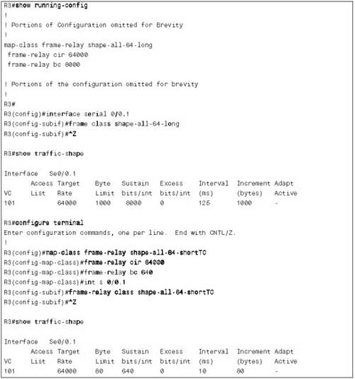
Example B-28 lists two configurations, with show command output listed after each configuration. In each case, the configuration commands enable you to explicitly set CIR, Bc, and Be, with Tc being calculated with the familiar Tc = Bc/CIR. In map-class frame-relay shape-all- 64-long, CIR and Bc are set to the same values as in the first FRTS configuration shown in Example B-27. After the configuration section at the beginning of Example B-28, this map class is enabled on interface S0/0.1; the show traffic-shape command now accurately lists the Bc value of 8000, and the shaping rate (as set by the frame-relay cir command) of 64,000 bps.
The second configuration in Example B-28 uses the map-class frame-relay shape-all-64- shortTC command to set Bc to 1/100 of the CIR value, which yields a Tc = 640/64,000, or 10 ms. This map class shows how you would set values to lower Tc, which is particularly useful to reduce the delay waiting for the next Tc if you have multiservice traffic. The example shows the configuration being changed to use map-class shape-all-64-shortTC by adding the frame- relay class shape-all-64-shortTC command. The show traffic-shape command follows, listing a Tc value of 10 ms.
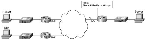
In Example B-29, the lab network has a new remote site added, with a PC named Kris, and a router (R2) with a 64-kbps CIR VC to R3. Suppose that the Frame Relay provider actually polices each VC at 96 kbps. The criteria for the configuration is summarized as follows:
![]() Shape all traffic from R3 to R1, and from R3 to R2, at 96 kbps.
Shape all traffic from R3 to R1, and from R3 to R2, at 96 kbps.
![]() Allow burst rates of 112 kbps on each VC.
Allow burst rates of 112 kbps on each VC.
![]() Use default settings for Bc and Be.
Use default settings for Bc and Be.
In this case, traffic to site R1 consists of a single VoIP call, and one web connection with two frames inside the page. At site R2, PC Kris FTP transfers a large file from the FTP server near R3. Figure B-22 shows the network, and Example B-29 shows the configuration and some sample show command output.
Example B-29 R3 FRTS Configuration on Two Different VCs, with Identical Settings
! Many lines omitted for brevity
!
interface Serial0/0
description connected to FRS port S0. Single PVC to R1.
no ip address
encapsulation frame-relay
load-interval 30
no fair-queue
clockrate 128000
frame-relay class shape-all-96
frame-relay traffic-shaping
!
interface Serial0/0.1 point-to-point
description point-point subint global DLCI 103, connected via PVC to DLCI 101 (
R1)
ip address 192.168.2.253 255.255.255.0
frame-relay interface-dlci 101
!
interface Serial0/0.2 point-to-point
description point-to-point subint connected to DLCI 102 (R2)
ip address 192.168.23.253 255.255.255.0
frame-relay interface-dlci 102
!
map-class frame-relay shape-all-96
frame-relay traffic-rate 96000 112000
no frame-relay adaptive-shaping
!
! Lines omitted for brevity
!
R3#show frame pvc 101
PVC Statistics for interface Serial0/0 (Frame Relay DTE)
DLCI = 101, DLCI USAGE = LOCAL, PVC STATUS = ACTIVE, INTERFACE = Serial0/0.1
input pkts 251070 output pkts 239522 in bytes 16004601
out bytes 34597106 dropped pkts 15567 in pkts dropped 0
out pkts dropped 15567 out bytes dropped 3005588
late-dropped out pkts 15567 late-dropped out bytes 3005588
in FECN pkts 0 in BECN pkts 0 out FECN pkts 0
out BECN pkts 0 in DE pkts 0 out DE pkts 0
out bcast pkts 1951 out bcast bytes 158000
pvc create time 02:22:11, last time pvc status changed 02:06:26
cir 96000 bc 96000 be 16000 byte limit 3500 interval 125
mincir 48000 byte increment 1500 Adaptive Shaping none
shaping inactive
traffic shaping drops 0
Queueing strategy: fifo
Output queue 0/40, 747 drop, 18449 dequeued
R3#show frame pvc 102
PVC Statistics for interface Serial0/0 (Frame Relay DTE)
DLCI = 102, DLCI USAGE = LOCAL, PVC STATUS = ACTIVE, INTERFACE = Serial0/0.2
input pkts 4063 output pkts 3820 in bytes 250312
out bytes 3863342 dropped pkts 1206 in pkts dropped 1206
out pkts dropped 0 out bytes dropped 0
in FECN pkts 0 in BECN pkts 0 out FECN pkts 0
out BECN pkts 0 in DE pkts 0 out DE pkts 0
out bcast pkts 587 out bcast bytes 50380
pvc create time 02:22:13, last time pvc status changed 02:05:29
cir 96000 bc 96000 be 16000 byte limit 3500 interval 125
mincir 48000 byte increment 1500 Adaptive Shaping none
pkts 2916 bytes 3802088 pkts delayed 1120 bytes delayed 1468724
shaping active
traffic shaping drops 0
Queueing strategy: fifo
Output queue 0/40, 0 drop, 1120 dequeued
R3#show traffic-shape
Interface Se0/0.1
Access Target Byte Sustain Excess Interval Increment Adapt
VC List Rate Limit bits/int bits/int (ms) (bytes) Active
101 96000 3500 96000 16000 125 1500 -
Interface Se0/0.2
Access Target Byte Sustain Excess Interval Increment Adapt
VC List Rate Limit bits/int bits/int (ms) (bytes) Active
102 96000 3500 96000 16000 125 1500 -
R3#show traffic-shape statistics
Access Queue Packets Bytes Packets Bytes Shaping
I/F List Depth Delayed Delayed Active
Se0/0.1 18 34730 4920740 19737 3510580 yes
Se0/0.2 0 3103 4065016 1191 1563968 yes
The FRTS configuration in this example sets FRTS parameters in a map class, which is then enabled on a physical interface. FRTS always performs shaping on each VC separately; therefore, in this case, the shaping parameters per VC will be picked up from the map class that has been enabled on the physical interface. Notice that a new map class, map-class shape-all-96, is configured with a frame-relay traffic-rate 96000 112000 command to set the CIR and EIR values. The frame-relay class shape-all-96 command has been added to the physical interface, and not to the individual subinterfaces. FRTS includes a feature that I call the inheritance feature, which just means that if a subinterface does not have a frame-relay class command, it uses the frame-relay class configured on the physical interface. Similarly, on multipoint subinterfaces, if a map class has not been configured on a particular DLCI, it inherits the FRTS parameters from the map class configured on the subinterface.
The first two show commands after the configuration (show frame pvc 101 and show frame pvc 102) list both shaping parameters and operational statistics. The parameters are the same, because each subinterface picked up its parameters from the map class (shape-all-96) that was enabled on the physical interface. However, the operational statistics differ, because FRTS shapes each VC separately. The show traffic-shape commands that follow confirm the same settings are used on each of the two subinterfaces as well. And in case you still think that FRTS may be shaping all the subinterfaces together, the show traffic-shape statistics command lists the varying statistics for shaping on each VC at the end of the example.
FRTS uses a default setting of CIR = 56 kbps, and Tc = 125 ms, if the frame-relay class command does not appear on the interface. In other words, if you enable FRTS on the physical interface with the frame-relay traffic-shape command, but do not enable a map class, FRTS still shapes each VC individually—but it does so with default parameters. So, be careful—pick a good set of default settings, put them in a map class, and enable it on the physical interface as in Example B-29, just to be safe.
In Example B-29, the G.729 voice call between R1 and R3 suffered, mainly due to the fact that shaping increases delay, and no effort was made to service the voice traffic more quickly. Suppose that the network engineer notices that IOS supports LLQ as an option for queuing in the shaping queues for FRTS. Therefore, he wants to solve the problem of poor voice quality by putting the voice call into a low-latency queue. With a shaping rate of 96 kbps, and with a single G.729 call, the voice call quality should improve. The criteria for the configuration is summarized as follows:
![]() Shape all traffic from R3 to R1, and from R3 to R2, at 96 kbps, respectively.
Shape all traffic from R3 to R1, and from R3 to R2, at 96 kbps, respectively.
![]() Use LLQ for queuing on the VC to R1, with 30 kbps maximum in the low-latency queue.
Use LLQ for queuing on the VC to R1, with 30 kbps maximum in the low-latency queue.
![]() Configure Bc so that Tc = 10 ms.
Configure Bc so that Tc = 10 ms.
![]() Use Be = 0.
Use Be = 0.
In this case, traffic to site R1 consists of a single VoIP call, and one web connection with two frames inside the page. At site R2, PC Kris FTP transfers a large file from the FTP server near R3. Example B-30 shows the configuration and some sample show commands.
Example B-30 FRTS to Two Sites, with LLQ Used in the Shaping Queue to Site 1
!
! Many lines omitted for brevity
!
class-map match-all voip-rtp
match ip rtp 16384 16383
!
policy-map voip-and-allelse
class voip-rtp
priority 30
!
interface Serial0/0
description connected to FRS port S0. Single PVC to R1.
no ip address
encapsulation frame-relay
load-interval 30
no fair-queue
clockrate 128000
frame-relay class shape-all-96
frame-relay traffic-shaping
!
interface Serial0/0.1 point-to-point
description point-point subint global DLCI 103, connected via PVC to DLCI 101 (
R1)
ip address 192.168.2.253 255.255.255.0
frame-relay class shape-with-LLQ
frame-relay interface-dlci 101
!
interface Serial0/0.2 point-to-point
description point-to-point subint connected to DLCI 102 (R2)
ip address 192.168.23.253 255.255.255.0
frame-relay interface-dlci 102
!
! Note No frame-relay class command on previous VC!
!
!
map-class frame-relay shape-all-96
frame-relay cir 96000
frame-relay bc 960
frame-relay be 0
!
frame-relay cir 96000
frame-relay bc 960
frame-relay be 0
service-policy output voip-and-allelse
!
R3#show frame-relay pvc 101
PVC Statistics for interface Serial0/0 (Frame Relay DTE)
DLCI = 101, DLCI USAGE = LOCAL, PVC STATUS = ACTIVE, INTERFACE = Serial0/0.1
input pkts 18487 output pkts 17749 in bytes 1184282
out bytes 2639555 dropped pkts 863 in pkts dropped 0
out pkts dropped 863 out bytes dropped 115649
late-dropped out pkts 863 late-dropped out bytes 115649
in FECN pkts 0 in BECN pkts 0 out FECN pkts 0
out BECN pkts 0 in DE pkts 0 out DE pkts 0
out bcast pkts 364 out bcast bytes 30272
pvc create time 00:26:08, last time pvc status changed 00:24:49
cir 96000 bc 96000 be 16000 byte limit 3500 interval 125
mincir 48000 byte increment 1500 Adaptive Shaping none
pkts 17718 bytes 2621259 pkts delayed 15671 bytes delayed 2238337
shaping active
traffic shaping drops 0
service policy voip-and-allelse
Serial0/0.1: DLCI 101 -
Service-policy output: voip-and-allelse
Class-map: voip-rtp (match-all)
5101 packets, 326464 bytes
30 second offered rate 25000 bps, drop rate 0 bps
Match: ip rtp 16384 16383
Weighted Fair Queueing
Strict Priority
Output Queue: Conversation 24
Bandwidth 30 (kbps) Burst 750 (Bytes)
(pkts matched/bytes matched) 4468/285952
(total drops/bytes drops) 0/0
Class-map: class-default (match-any)
386 packets, 412201 bytes
30 second offered rate 31000 bps, drop rate 0 bps
Match: any
Output queue size 42/max total 600/drops 0
R3#show traffic-shape queue serial 0/0.1
Queueing strategy: weighted fair
Queueing Stats: 15/600/64/0 (size/max total/threshold/drops)
Conversations 4/8/16 (active/max active/max total)
Reserved Conversations 0/0 (allocated/max allocated)
Available Bandwidth 18 kilobits/sec
(depth/weight/total drops/no-buffer drops/interleaves) 5/0/0/0/0
Conversation 24, linktype: ip, length: 64
source: 192.168.3.254, destination: 192.168.2.251, id: 0x012F, ttl: 253,
TOS: 0 prot: 17, source port 19018, destination port 17766
(depth/weight/total drops/no-buffer drops/interleaves) 3/32384/0/0/0
Conversation 2, linktype: ip, length: 1404
source: 192.168.3.100, destination: 192.168.1.100, id: 0x177B, ttl: 127,
TOS: 0 prot: 6, source port 80, destination port 1148
(depth/weight/total drops/no-buffer drops/interleaves) 2/32384/0/0/0
Conversation 1, linktype: ip, length: 1404
source: 192.168.3.100, destination: 192.168.1.100, id: 0x1775, ttl: 127,
TOS: 0 prot: 6, source port 80, destination port 1147
(depth/weight/total drops/no-buffer drops/interleaves) 5/32384/0/0/0
Conversation 12, linktype: ip, length: 1244
source: 192.168.3.100, destination: 192.168.1.100, id: 0x1758, ttl: 127,
TOS: 0 prot: 6, source port 1176, destination port 1146
R3#sh traffic-shape queue s 0/0.2
Traffic queued in shaping queue on Serial0/0.2 dlci 102
Queueing strategy: fcfs
Example B-30 begins with the new FRTS and LLQ configuration. The policy-map voip-and-allelse command defines a policy map that puts all even RTP ports into a low-latency queue, with 32 kbps maximum, and all other traffic into the class-default class. LLQ is enabled inside a new FRTS map-class shape-with-LLQ command, with the service-policy output voip-and- allelse command enabling LLQ inside the map class. Any VC that uses the shape-with-LLQ map class will use the settings in that map class, including the LLQ configuration. In this case, the single VC on subinterface s 0/0.1 uses LLQ for the shaping queue because of the frame- relay class shape-with-LLQ command.
The VC on subinterface S0/0.2 does not use map-class voip-and-allelse. Because no frame- relay class command is configured on subinterface 0/0.2, FRTS uses the shaping parameters from map-class shape-all-64, because it is configured on physical interface s 0/0.
Immediately following the configuration, the show frame-relay pvc 101 command lists a large amount of new information. Essentially, IOS lists the same kinds of information normally seen with the show policy-map interface command in the show frame-relay pvc 101 command. Information about the MQC classes defined, and statistics about the packets in each class, is listed. Also note that the show traffic-shape queue s 0/0.2 at the end of the example reminds us that FCFS is used on the other subinterface.
If you take a step back from the configuration and show commands for a moment, it may be obvious that the two VCs, shaped at 96 kbps each, oversubscribe R3’s access link, which is clocked at 128 kbps. Because FRTS only supports FIFO Queuing on the physical interface, congestion still occurs there. Although adding LLQ to subinterface S0/0.1 helped the quality of the voice call, call quality still suffered due to drops and jitter caused by the oversubscribed FIFO output queue on the physical interface s 0/0.
The final solution to the voice quality problem in this case is to take advantage of the queuing feature introduced by FRF.12 fragmentation. Frame Relay fragmentation (FRF) can be used with FRTS. FRF actually creates a set of two queues on the physical interface, called dual-FIFO queues. Packets that are larger than the fragmentation size are fragmented and placed into one queue. Packets that are equal to, or smaller than, the fragmentation size are not fragmented, and placed into the other queue. IOS treats the nonfragmented frame queue as a priority queue—in other words, it is always serviced first. Therefore, if you want to give great service to small packets such as VoIP, FRF can provide the traditional benefits of fragmentation, and provide a priority queue for all small packets, including VoIP. Figure B-23 outlines the basic idea, with FRTS on two subinterfaces.

Using FRF to create a two-queue PQ system works well with voice traffic, because the packets are generally small. However, video traffic includes too many larger packets to benefit substantially from FRF’s queuing feature, because the larger packets are fragmented and placed in the lower-priority queue. Chapter 8, “Link Efficiency Tools,” shows the configuration for adding FRF to this network.
Other FRTS configuration items that might be on the exam include how to configure adaptive shaping, and how to enable FRTS parameters on a VC on a multipoint subinterface. Example B-31 lists a simple map class configuration that enables adaptive shaping, with the configuration added to DLCI 101, but not DLCI 102, on multipoint subinterface S0/0.33.
Example B-31 FRTS Adaptive Shaping and per-DLCI Configuration
!
! Many lines omitted for brevity
!
interface Serial0/0
description connected to FRS port S0. Single PVC to R1.
no ip address
encapsulation frame-relay
load-interval 30
no fair-queue
clockrate 128000
frame-relay class shape-all-96
frame-relay traffic-shaping
!
interface Serial0/0.33 multipoint
description multipoint subint, w/ DLCIs 101 and 102
ip address 192.168.2.253 255.255.255.0
frame-relay interface-dlci 101
class my-adapt-shape-class
frame-relay interface-dlci 102
!
map-class frame-relay shape-all-96
frame-relay traffic-rate 96000 112000
!
map-class frame-relay my-adapt-shape-class
frame-relay traffic-rate 96000 112000
frame-relay adaptive-shaping becn
frame-relay mincir 64000
The map-class frame-relay my-adapt-shape-class command creates a new map class with adaptive FRTS enabled. With adaptive shaping, FRTS uses the shape rate as the maximum rate, and the rate configured on the frame-relay mincir command as the minimum rate. The new map-class my-adapt-shape-class command enables adaptive shaping with the frame-relay adaptive-shaping becn command, and sets the mincir with the frame-relay mincir 64000 command. The map class is enabled on DLCI 101, but not DLCI 102, on subinterface s0/0.33.
The example also shows how to enable a map class for a single DLCI. To enable an FRTS map class per DLCI, first enter subinterface configuration mode, and then issue the frame-relay interface-dlci command. This command places you into DLCI configuration mode, where the class my-adapt-shape-class command enables map class my-adapt-shape-class just for this DLCI. Note that after the frame-relay interface-dlci 102 command, there is no class command. So, on DLCI 102, the FRTS parameters in class shape-all-96, as configured on the physical interface, are used.
Table B-33 summarizes the key points for comparison between the various traffic-shaping tools, highlighting FRTS.
CAR has more similarities than differences when compared to CB policing. Both perform policing on all traffic on either an interface or subinterface. Both can classify traffic to police a subset of traffic as well. Both use the same units when configuring policing parameters—bits per second for the policing rate, bytes for the normal and Be values, with the configured Be value actually representing Bc + Be.
CAR differs from CB policing regarding four main features. The most obvious is that CAR uses the rate-limit command, which is not part of the MQC set of commands. CAR also uses only two categories for actions—conform and exceed—as opposed to the three categories (conform, exceed, and violate) supported by CB policing. The most significant difference is that CAR has a feature called cascaded or nested rate-limit commands. Finally, CAR does not use MQC for configuration. Each of these differing features are covered in the example configurations.
Most QoS tools that classify packets operate with logic similar to ACLs in that, when a packet is matched, the action(s) related to that matched statement are taken. With all MQC features, such as CB marking, CBWFQ, CB policing, and CB shaping, after a particular class has been matched, the action associated with that class inside the policy map is performed. For instance, all MQC policy maps end with the class-default class, which matches all packets; however, packets may have matched an earlier class, so that a packet would never fall through to the class-default class.
With CAR, a single packet can match multiple statements. By doing so, you can actually police progressively more specific subsets of the traffic on the interface or subinterface. For example, you can create logic such as the following:
![]() Police all traffic on the interface at 500 kbps; but before sending this traffic on its way ...
Police all traffic on the interface at 500 kbps; but before sending this traffic on its way ...
![]() Police all web traffic at 400 kbps.
Police all web traffic at 400 kbps.
![]() Police all FTP traffic at 150 kbps
Police all FTP traffic at 150 kbps
![]() Police all VoIP traffic at 200 kbps.
Police all VoIP traffic at 200 kbps.
In other words, you can police a larger group of traffic, but also prevent one particular subset of that group from taking over all the available bandwidth. For example, CAR can be configured so thatweb traffic can only take 400 kbps of the traffic, but the overall rate can be 500 kbps. This section ends with a configuration example that polices a larger set of traffic, and subsets of the larger set.
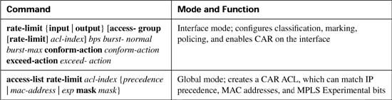
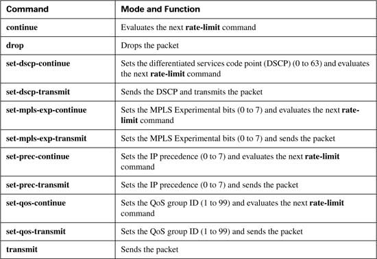
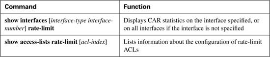
Table B-34 lists the configuration commands used with CAR, and Table B-35 lists the options for the actions to be taken when CAR decides a packet either conforms to or exceeds the traffic contract. Table B-36 lists the CAR show commands.
Like CB policing, you can use CAR to police all traffic entering or exiting an interface. In Example B-32, router ISP-edge polices ingress traffic from an enterprise network. The criteria for the first CB policing example is as follows:
![]() All traffic policed at 96 kbps at ingress to the ISP-edge router.
All traffic policed at 96 kbps at ingress to the ISP-edge router.
![]() Bc of 1 second’s worth of traffic is allowed.
Bc of 1 second’s worth of traffic is allowed.
![]() Be of 0.5 second’s worth of traffic is allowed.
Be of 0.5 second’s worth of traffic is allowed.
![]() Traffic that exceeds the contract is discarded.
Traffic that exceeds the contract is discarded.
![]() Traffic that conforms to the contract is forwarded with precedence reset to zero.
Traffic that conforms to the contract is forwarded with precedence reset to zero.
Figure B-24 shows the network in which the configuration is applied, and Example B-32 shows the configuration.

Example B-32 CB Policing at 96 kbps at ISP-edge Router
!
!Lines omitted for brevity
!
interface Serial1/0
description connected to FRS port S1. Single PVC to R3.
no ip address
encapsulation frame-relay
load-interval 30
no fair-queue
clockrate 1300000
!
interface Serial1/0.1 point-to-point
description point-point subint global DLCI 101, connected via PVC to DLCI 103 (R3)
ip address 192.168.2.251 255.255.255.0
! note: the rate-limit command wraps around to a second line.
rate-limit input 96000 12000 18000 conform-action set-prec-transmit 0
exceed-action drop
frame-relay interface-dlci 103
!
!Lines omitted for brevity
!
ISP-edge#show interfaces s 1/0.1 rate-limit
Serial1/0.1 point-point subint global DLCI 101, connected via PVC to DLCI 103 (R3)
Input
matches: all traffic
params: 96000 bps, 12000 limit, 18000 extended limit
conformed 2290 packets, 430018 bytes; action: set-prec-transmit 0
exceeded 230 packets, 67681 bytes; action: drop
last packet: 0ms ago, current burst: 13428 bytes
last cleared 00:02:16 ago, conformed 25000 bps, exceeded 3000 bps
ISP-edge#
The configuration requires a single rate-limit command under serial 1/0.1 on router ISP-edge. All the parameters are typed in the single command line: rate-limit input 96000 12000 18000 conform-action set-prec-transmit 0 exceed-action drop. The rate of 96 kbps is listed with a Bc of 12,000 bytes, and a Be of 6000 bytes. (Remember, the burst-excess parameter of 18,000 is actually Bc + Be.)
The show interfaces s1/0.1 rate-limit command lists the operational statistics, including numbers of bytes and packets that conformed and exceeded the contract. Interestingly, the two measured rates (conform and exceed) over time do not total more than the policing rate; it appears that the preemptive discarding of packets with the debt process during Be processing is having some good effect. In this particular network, only three concurrent TCP connections were used to create traffic, so just a few packets lost would reduce the TCP windows, and reduce traffic quickly.
Example B-33 exhibits how to classify traffic with CAR using rate-limit ACLs, and how to use CAR with cascaded rate-limit commands. To classify traffic, CAR requires the use of either a normal ACL, or a rate-limit ACL. A rate-limit ACL can match MPLS Experimental bits, IP precedence, or MAC address. For CAR to match other IP header fields, you must use an IP ACL. In Example B-33, the CAR configuration meets the requirements of the example for cascaded statements mentioned in the introduction to this section, repeated in the following list.
![]() Police all traffic on the interface at 496 kbps; but before sending this traffic on its way ...
Police all traffic on the interface at 496 kbps; but before sending this traffic on its way ...
![]() Police all web traffic at 400 kbps.
Police all web traffic at 400 kbps.
![]() Police all FTP traffic at 160 kbps
Police all FTP traffic at 160 kbps
![]() Police all VoIP traffic at 200 kbps.
Police all VoIP traffic at 200 kbps.
![]() Choose Bc and Be so that Bc has 1 second’s worth of traffic, and Be provides no additional burst capability over Bc.
Choose Bc and Be so that Bc has 1 second’s worth of traffic, and Be provides no additional burst capability over Bc.
Example B-33 shows the configuration.
Example B-33 Cascaded CAR rate-limit Commands, with Subclassifications
! Next ACL matches all web traffic
!
Access-list 101 permit tcp any eq www any
Access-list 101 permit tcp any any eq www
!
! Next ACL matches all FTP traffic
!
access-list 102 permit tcp any eq ftp any
access-list 102 permit tcp any any eq ftp
access-list 102 permit tcp any eq ftp-data any
access-list 102 permit tcp any any eq ftp-data
!
! Next ACL matches all VoIP traffic
!
access-list 103 permit udp any range 16384 32767 any range 16384 32767
!
interface s 0/0
rate-limit input 496000 62000 62000 conform-action continue exceed-action drop
rate-limit input access-group 101 400000 50000 50000 conform-action transmit exceed- action
drop
rate-limit input access-group 102 160000 20000 20000 conform-action transmit exceed- action
drop
rate-limit input access-group 103 200000 25000 25000 conform-action transmit exceed- action
drop
The CAR configuration needs to refer to IP ACLs to classify the traffic, using three different IP ACLs in this case. ACL 101 matches all web traffic, ACL 102 matches all FTP traffic, and ACL 103 matches all VoIP traffic.
Under subinterface S1/0.1, four rate-limit commands are used. The first sets the rate for all traffic, dropping traffic that exceeds 496 kbps. However, the conform action is listed as “continue”. This means that packets conforming to this statement are now compared to the next rate-limit statements, and when matching a statement, some other action is taken. For instance, web traffic matches the second rate-limit command, with a resulting action of either transmit or drop. VoIP traffic is actually compared with the next three rate-limit commands before matching the last rate-limit command. The following list characterizes the types of traffic, and which rate-limit commands they match, in the example.
![]() All traffic matches the first rate-limit command, and is either dropped or passed to the second rate-limit command.
All traffic matches the first rate-limit command, and is either dropped or passed to the second rate-limit command.
![]() All web traffic matches the second rate-limit command, and is either transmitted or dropped.
All web traffic matches the second rate-limit command, and is either transmitted or dropped.
![]() All FTP traffic matches the third rate-limit command, and is either transmitted or dropped.
All FTP traffic matches the third rate-limit command, and is either transmitted or dropped.
![]() All VoIP traffic matches the fourth rate-limit command, and is either transmitted or dropped.
All VoIP traffic matches the fourth rate-limit command, and is either transmitted or dropped.
![]() All other traffic is transmitted, because it did not match any more rate-limit commands.
All other traffic is transmitted, because it did not match any more rate-limit commands.
You also may have noticed that the policing rates used in this example did not exactly match the values in the original problem statement at the beginning of this section. For instance, originally the requirement stated 500 kbps for all traffic; the configuration uses 496 kbps. CAR requires that the policing rate be a multiple of 8000, so the requirements were adjusted accordingly.
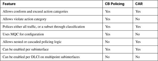
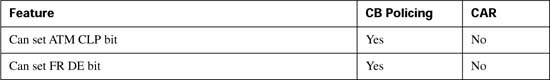
Table B-37 summarizes the CAR features, comparing them with CB policing.
This section covers Flow-Based Random Early Detection (FRED).
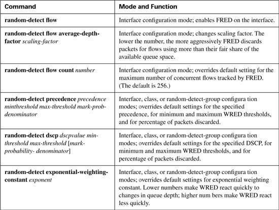
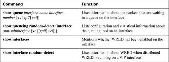
FRED configuration requires only slightly more effort than does WRED configuration, as long as default configuration values are acceptable. This section shows two FRED configuration examples that involve the same basic scenarios as the first two WRED examples in the previous section. FRED configuration and show commands are listed in Tables B-38 and B-39.
In the first example, R3 enables FRED on its S0/0 interface. FRED classifies the packets into flows and then decides which flows are currently considered to be robust, fragile, and nonadaptive. Based on the category, FRED decides whether new packets should be discarded.
This example continues the tradition of marking packets at ingress on R3’s E0/0 interface. The marking logic performed by CB marking is as follows:
![]() VoIP payload—DSCP EF
VoIP payload—DSCP EF
![]() HTTP traffic for web pages with “important” in the URL—DSCP AF21
HTTP traffic for web pages with “important” in the URL—DSCP AF21
![]() HTTP traffic for web pages with “not-so” in the URL—DSCP AF23
HTTP traffic for web pages with “not-so” in the URL—DSCP AF23
![]() All other—DSCP default
All other—DSCP default
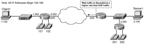
To generate traffic in this network, two voice calls will be made between the analog phones attached to R1 and R4. Multiple web browsers will load the standard page used in this book, with two TCP connections created by each browser—one to get a file with the word “important” in it, and the other getting a file with “not-so” in it. An FTP download of a large file will also be initiated from the Server to Client1. Example B-34 shows the basic configuration and show command output. The example uses the familiar network diagram in Figure B-25, with the configuration being added to R3.
Example B-34 FRED Example Using All Default Values, R3 S0/0
Building configuration...
!
! Some lines omitted for brevity
!
ip cef
!
! The following class-maps will be used for CB marking policy
! used at ingress to E0/0
!
class-map match-all http-impo
match protocol http url "*important*"
class-map match-all http-not
match protocol http url "*not-so*"
class-map match-all class-default
match any
class-map match-all voip-rtp
match ip rtp 16384 16383
!
! The following policy-map will be used for CB marking
!
policy-map laundry-list
class voip-rtp
set ip dscp ef
class http-impo
set ip dscp af21
class http-not
set ip dscp af23
class class-default
set ip dscp default
!
!
interface Ethernet0/0
description connected to SW2, where Server1 is connected
ip address 192.168.3.253 255.255.255.0
ip nbar protocol-discovery
half-duplex
service-policy input laundry-list
!
interface Serial0/0
description connected to FRS port S0. Single PVC to R1.
no ip address
encapsulation frame-relay
load-interval 30
random-detect
random-detect flow
clockrate 128000
!
interface Serial0/0.1 point-to-point
description point-point subint global DLCI 103, connected via PVC to DLCI 101 (
R1)
ip address 192.168.2.253 255.255.255.0
frame-relay interface-dlci 101
!
!
! Some lines omitted for brevity
!
R3#show queueing random-detect
Current random-detect configuration:
Serial0/0
Exp-weight-constant: 9 (1/512)
Mean queue depth: 36
Max flow count: 256 Average depth factor: 4
Flows (active/max active/max): 2/8/256
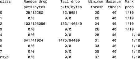
The FRED part of the configuration is again quite short. The configuration lists the random- detect interface subcommand under serial 0/0, which enables precedence-based WRED on the interface. Because FRED is actually a superset of WRED, you also need to add the random- detect flow command to the interface. Interestingly, IOS adds the random-detect command to the interface if you only type the random-detect flow command. The rest of the detailed configuration in this example is just like the first WRED example configuration, repeating the CB marking configuration that marks the VoIP, FTP, and two different types of HTTP traffic. (For more information about CB marking, see Chapter 3.)
The only command that lists any new information, as compared with WRED, is the show queueing random-detect interface serial 0/0 command. Most of the output looks familiar: It includes the various IP precedence values, with statistics. Just like with WRED, the command lists per-precedence default values for minimum threshold and maximum threshold. FRED still uses these values when determining the percentage of packets to discard. Specifically new for FRED, the command output lists two values used by the FRED algorithm when deciding to discard packets, namely the maximum flow count and average depth factor. The maximum flow count is the maximum number of unique active flows tracked by FRED. The average depth factor describes the scaling factor as described in the FRED concepts section, used when calculating the maximum per-flow queue size.
Although FRED does track and act on flow information, listing statistics per flow would be cumbersome, because the flows may well be short lived. The show queueing command still lists statistics, but it groups the statistics based on the precedence value (or DSCP value if DSCP-based FRED is used).
The second FRED configuration example uses FRED on the interface again, but this time with DSCP FRED, and a few defaults changed. In fact, Example B-35 just shows the changed configuration, with most of the configuration staying the same. The same CB marking configuration is used to mark the traffic, for instance, so the details are not repeated in the example. The example uses the familiar network diagram used in Figure B-25.
Example B-35 DSCP-Based FRED on R3 S0/0
Enter configuration commands, one per line. End with CNTL/Z.
R3(config)#interface serial 0/0
R3(config-if)#random-detect flow ?
average-depth-factor Average depth multiplier (1, 2, 4, 8 or 16)
count max number of dynamic flows
<cr>
R3(config-if)#random-detect flow average-depth-factor 2
R3(config-if)#random-detect flow count 19
Number of WRED flows must be a power of 2 (16, 32, 64, 128, 256, 512, 1024
R3(config-if)#random-detect flow count 64
R3(config-if)#^Z
R3#
R3#show queueing random-detect
Current random-detect configuration:
Serial0/0
Queueing strategy: random early detection (WRED)
Exp-weight-constant: 9 (1/512)
Mean queue depth: 39
Max flow count: 64 Average depth factor: 2
Flows (active/max active/max): 13/13/64

The configuration begins with a change from precedence-based FRED to DSCP-based FRED using the random-detect dscp-based interface subcommand. (The configuration already contained the random-detect flow command to enable flow-based WRED.) Two FRED options can be set with the random-detect flow command, as seen in the example. The average depth factor defines the multiple of the average queue space per flow that can be allocated to a single flow before FRED decides to start discarding packets. (Formula: average depth factor * maximum queue depth / number of active flows) The flow count, set to 64 in this example, just sets the maximum number of unique flows tracked by FRED. Just like with WFQ, the setting of the number of flows must be set to a power of 2.
Just like with DSCP-based WRED, the command output for DSCP-based FRED does not differ from the earlier precedence-based FRED example in too many ways. The changes to the default values have been highlighted in the example. The show queueing command contains the only notable difference between the command outputs in the first two examples, now listing information about all the DSCP values recommended in the DSCP RFCs. Notice that the counters point out drops for both AF21 and AF23, which were previously both treated as precedence 2 by precedence-based FRED. Also note that FRED has discarded some voice traffic (DSCP EF) in this example. Because FRED operates on all traffic in the interface FIFO queue, it cannot avoid the possibility of discarding voice traffic.
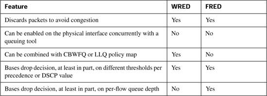
Table B-40 summarizes many of the key concepts when comparing WRED and FRED.
This section covers Payload Compression configuration, RTP and TCP header compression configuration (without MQC), and a comparison of FRF.11-C and FRF.12 fragmentation.
Payload compression requires little configuration. You must enable compression on both ends of a point-to-point serial link, or on both ends of a Frame Relay VC for Frame Relay. The compress command enables compression on point-to-point links, with the frame-relay payload-compression command enabling compression over Frame Relay.
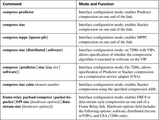
Table B-41 lists the various configuration and show commands used with payload compression, followed by example configurations.
You can use the show compress command to verify that compression has been enabled on the interface and to display statistics about the compression behavior.
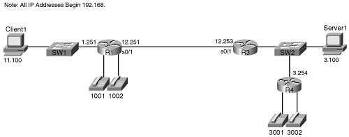
The first example uses the network described in Figure B-26, with a PPP link between R1 and R3. The example uses the same familiar web browsing sessions, each of which downloads two JPGs. An FTP get transfers a file from the server to the client, and two voice calls between R1 and R4 are used.
Example B-36 shows the Stacker compression between R1 and R3.
Example B-36 Stacker Payload Compression Between R1 and R3 (Output from R3)
Building configuration...
!
! Lines omitted for brevity
!
interface Serial0/1
bandwidth 128
ip address 192.168.12.253 255.255.255.0
encapsulation ppp
compress stacker
clockrate 128000
!
! Portions omitted for brevity
!
r3#show compress
Serial0/1
Software compression enabled
uncompressed bytes xmt/rcv 323994/5494
compressed bytes xmt/rcv 0/0
1 min avg ratio xmt/rcv 1.023/1.422
5 min avg ratio xmt/rcv 1.023/1.422
10 min avg ratio xmt/rcv 1.023/1.422
no bufs xmt 0 no bufs rcv 0
resyncs 2
The configuration requires only one interface subcommand, compress stacker. You must enter this command on both ends of the serial link before compression will work. The show compress command lists statistics about how well compression is working. For instance, the 1-, 5-, and 10-minute compression ratios for both transmitted and received traffic are listed, which gives you a good idea of how much less bandwidth is being used because of compression.
You can easily configure the other two payload compression tools. Instead of the compress stacker command as in Example B-36, just use the compress mppc or compress predictor command.
Example B-37 shows FRF.9 payload compression. The configuration uses a point-to-point subinterface and the familiar network used on most of the other configuration examples in the book, as shown in Figure B-27.
Example B-37 FRF.9 Payload Compression Between R1 and R3 (Output from R3)
Building configuration...
!
! Lines omitted for brevity
!
description Single PVC to R1.
no ip address
encapsulation frame-relay IETF
no ip mroute-cache
load-interval 30
clockrate 128000
!
interface Serial0/0.1 point-to-point
description point-point subint global DLCI 103, connected via PVC to DLCI 101 (R1)
ip address 192.168.2.253 255.255.255.0
no ip mroute-cache
frame-relay interface-dlci 101 IETF
frame-relay payload-compression FRF9 stac
!
! Portions omitted for brevity
!
R3#show compress
Serial0/0 - DLCI: 101
Software compression enabled
uncompressed bytes xmt/rcv 6480/1892637
compressed bytes xmt/rcv 1537/1384881
1 min avg ratio xmt/rcv 0.021/1.352
5 min avg ratio xmt/rcv 0.097/1.543
10 min avg ratio xmt/rcv 0.097/1.543
no bufs xmt 0 no bufs rcv 0
resyncs 1
Additional Stacker Stats:
Transmit bytes: Uncompressed = 0 Compressed = 584
Received bytes: Compressed = 959636 Uncompressed = 0
Frame Relay payload compression takes a little more thought, although it may not be apparent from the example. On point-to-point subinterfaces, the frame-relay payload-compression FRF9 stac command enables FRF.9 compression on the VC associated with the subinterface. If a multipoint subinterface is used, or if no subinterfaces are used, however, you must enable compression as parameters on the frame-relay map command.
Unlike payload compression, Cisco IOS Software does not have different variations on the compression algorithms for TCP and RTP header compression. To enable TCP or RTP compression, you just enable it on both sides of a point-to-point link, or on both sides of a Frame Relay VC.
Note that when enabling compression, it is best practice to enable the remote side of the WAN link before enabling the local side of the WAN link. This enables the administrator to retain control of WAN connectivity. If the local side of the WAN link is configured first, an out-of-band access must exist to access the remote side.
When configuring Frame Relay TCP or RTP header compression, the style of configuration differs based on whether you use point-to-point subinterfaces. On point-to-point subinterfaces, the frame-relay ip tcp or frame-relay ip rtp commands are used. If you use multipoint subinterfaces, or use the physical interface, you must configure the same parameters on frame-relay map commands.
Regardless of the type of data-link protocol in use, TCP and RTP compression commands allow the use of the passive keyword. The passive keyword means that the router attempts to perform compression only if the router on the other side of the link or VC compresses the traffic. The passive keyword enables you to deploy configurations on remote routers with the passive keyword, and then later add the compression configuration on the local router, at which time compression begins.
The TCP and RTP header compression configuration process, as mentioned, is very simple. Table B-42 and Table B-43 list the configuration and show commands, which are followed by a few example configurations.
The first example uses the same point-to-point link used in the payload compression section, as shown earlier in Figure B-26. In each example, the same familiar web browsing sessions are used, each downloading two JPGs. An FTP get transfers a file from the server to the client, and two voice calls between R1 and R4 are used.
Example B-38 shows TCP header compression on R3.
Example B-38 TCP Header Compression on R3
Building configuration...
!
! Lines omitted for brevity
!
interface Serial0/1
bandwidth 128
ip address 192.168.12.253 255.255.255.0
encapsulation ppp
ip tcp header-compression
clockrate 128000
!
! Portions omitted for brevity
!
R3#show ip tcp header-compression
TCP/IP header compression statistics:
Interface Serial0/1:
Rcvd: 252 total, 246 compressed, 0 errors
0 dropped, 0 buffer copies, 0 buffer failures
Sent: 371 total, 365 compressed,
12995 bytes saved, 425880 bytes sent
1.3 efficiency improvement factor
Connect: 16 rx slots, 16 tx slots,
218 long searches, 6 misses 0 collisions, 0 negative cache hits
98% hit ratio, five minute miss rate 0 misses/sec, 1 max
To enable TCP header compression, the ip tcp header-compression command was added to both serial interfaces on R1 and R3. The show ip tcp header-compression command lists statistics about how well TCP compression is working. For instance, 365 out of 371 packets sent were compressed, with a savings of 12,995 bytes. Interestingly, to find the average number of bytes saved for each of the compressed packets, divide the number of bytes saved (12,995) by the number of packets compressed (365), which tells you the average number of bytes saved per packet was 35.6. For comparison, remember that TCP header compression reduces the 40 bytes of IP and TCP header down to between 3 and 5 bytes, meaning that TCP header compression should save between 35 and 37 bytes per packet, as is reflected by the output of the show ip tcp header-compression command.
To configure RTP header compression on point-to-point links, you perform a similar exercise as you did for TCP in Example B-38, except you use the rtp keyword rather than the tcp keyword to enable RTP header compression. For a little variety, however, the next example shows RTP header compression, as enabled on a Frame Relay link between R3 and R1. The network used in this example matches Figure B-27, shown in the Frame Relay payload compression example. Example B-39 shows the configuration and statistics.
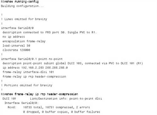
To enable RTP header compression, the frame-relay ip rtp header-compression command was added to both serial subinterfaces on R1 and R3. (If a multipoint subinterface had been used instead, the same parameters could have been configured on a frame-relay map command.)
The show frame-relay ip rtp header-compression command lists statistics about how well cRTP is working. You might recall that cRTP reduces the 40 bytes of IP, UDP, and RTP header to between 2 and 4 bytes, saving between 36 and 38 bytes per packet. In the output in the example, with 16,992 packets compressed, a savings of 645,645 bytes is realized, which is an average per-packet savings of 37.99 bytes.
The show frame-relay ip rtp header-compression command output also lists an efficiency improvement factor, which is the compression ratio. It is calculated as the number of bytes that would have been sent without compression, divided by the actual number of bytes sent. From the shaded lines at the end of the preceding example, 645,645 + 373,875 bytes would have been sent (the number of bytes saved, plus actual number sent), for a total of 1,019,520 bytes that would have been sent. Dividing that total by the actual number sent (373,875) gives you the improvement factor of 2.72. For perspective, if you divide the packet size of a G.729 VoIP packet (60 bytes), by the compressed size of 22 bytes (which implies you saved 38 of the 40 bytes in the header), the ratio also calculates to 2.72. Therefore, the empirical ratio from the show command matches the theoretical ratio between bytes that would have been sent, and bytes that are actually sent, with cRTP.
Most of the coverage of LFI over Frame Relay has focused on FRF.12. However, IOS offers another Frame Relay LFI service called FRF.11-C. You can use each of these two LFI options only when you use particular types of Frame Relay VCs. To appreciate how the two options differ, you first need to understand these two types of VCs.
The Frame Relay Forum (FRF) created data VCs originally to carry multiprotocol data traffic, as defined in the FRF.3 Implementation Agreements. Service providers around the world offer Frame Relay FRF.3 data VCs.
Later, with the advent of packetized voice, the Frame Relay Forum decided to create a new type of VC that would allow for better treatment of voice traffic. The FRF created the FRF.11
Implementation Agreement, which defines Voice over Frame Relay (VoFR) VCs. These VCs still pass data traffic, but they also pass voice traffic. Therefore, if a Frame Relay switch knows that one frame is data, and another is voice, for example, the switch can implement some form of queuing to give the voice frame low latency. FRF.11 headers include a field that identifies the frame as voice or data, making it possible for the cloud to perform QoS for the voice traffic.
The key to understanding the difference between the two basic types of VCs is to look at the headers used when the frames cross the Frame Relay network. It helps to understand when VoFR VCs can be useful, and when they cannot. Figure B-28 shows the framing when FRF.3 and FRF.11 are used, both for IP telephony traffic and for local voice gateway traffic.
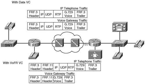
In all cases in the figure, G.729 codecs are used. With FRF.3 VCs, the IP Phone and voice gateway traffic sits inside IP/UDP/RTP headers. In other words, the IP Phones encapsulate the G.729 payload using VoIP, and the routers do the same for the analog and digital voice trunks. Although the packets traverse the Frame Relay network, all the voice traffic is considered to be VoIP traffic when you use FRF.3 data VCs.
With FRF.11 VCs, some voice traffic can be VoIP, and some can be VoFR traffic. The traffic to and from the directly attached analog and digital voice links can be encapsulated using VoFR, as shown in the lowest of the four example frames. The IP telephony traffic, however, still must be encapsulated first in IP, because the traffic must pass across other links besides this single Frame Relay cloud. The VoFR encapsulation requires far less overhead, because the IP, RTP, and UDP headers are not needed. However, VoFR you can use encapsulation only when the Frame Relay-attached routers are the endpoints for the packets holding the voice payload. Because the larger percentage of packetized voice over time will be from IP Phones and the like, VoFR services are not typically offered by Frame Relay providers.
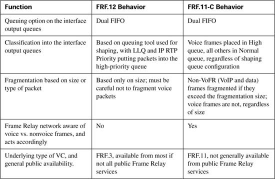
FRF.11-C provides for LFI over VoFR VCs, similarly to how FRF.12 provides LFI services for FRF.3 data VCs. Just like FRF.12, FRF.11-C uses Dual FIFO interface output queues, with PQ logic applied to the two queues. However, FRF.11-C uses a different classification logic, as follows:
![]() VoFR frames are placed into the High queue on the interface.
VoFR frames are placed into the High queue on the interface.
![]() All data frames are placed into the Normal queue.
All data frames are placed into the Normal queue.
In the preceding figure, the VoFR frames created for the voice gateway would be placed in the High queue, but the IP Phone packets would be placed into the Normal queue, because they would be considered to be data.
The other main difference between FRF.11-C and FRF.12 has to do with how the tools decide what to fragment, and what not to fragment. FRF.12 fragments all packets over a certain length. FRF.11-C, however, never fragments VoFR frames, even if they are larger than the fragment size. FRF.11-C fragments data frames only, and only if they are larger than the fragment size.
Table B-44 summarizes some of the key comparison points about FRF.12 and FRF.11-C.