Chapter 6. Traffic Policing and Shaping
QoS Exam Objectives
This chapter covers the following exam topics specific to the QoS exam:
![]() Describe the purpose of traffic conditioning using traffic policing and traffic shaping and differentiate between the features of each
Describe the purpose of traffic conditioning using traffic policing and traffic shaping and differentiate between the features of each
![]() Explain how network devices measure traffic rates using single rate or dual rate, single or dual token bucket mathematical models
Explain how network devices measure traffic rates using single rate or dual rate, single or dual token bucket mathematical models
![]() Identify the Cisco IOS commands required to configure and monitor single rate and dual rate CB-Policing
Identify the Cisco IOS commands required to configure and monitor single rate and dual rate CB-Policing
![]() Identify the Cisco IOS commands required to configure and monitor percentage based CB-Policing
Identify the Cisco IOS commands required to configure and monitor percentage based CB-Policing
![]() Explain how the two rate limits, average rate and peak rate, can be used to rate limit traffic
Explain how the two rate limits, average rate and peak rate, can be used to rate limit traffic
![]() Identify the Cisco IOS commands required to configure and monitor CB-Shaping
Identify the Cisco IOS commands required to configure and monitor CB-Shaping
![]() Identify the Cisco IOS commands required to configure and monitor Frame Relay adaptive CB-Shaping on Frame Relay interfaces
Identify the Cisco IOS commands required to configure and monitor Frame Relay adaptive CB-Shaping on Frame Relay interfaces
Traffic policing allows devices in one network to enforce a traffic contract. Traffic contracts define how much data one network can send into another, typically expressed as a committed information rate (CIR) and a committed burst (Bc). Policing measures the flow of data, and discards packets that exceed the traffic contract.
Similarly, traffic shaping allows packets to conform to a traffic contract. In cases where packets that exceed the traffic contract might be discarded, the sending device may choose just to slow down its sending rate, so that the packets are not discarded. The process of sending the traffic more slowly than it could be sent, to conform to a traffic contract, is called shaping.
In short, policing typically drops out-of-contract traffic, whereas shaping typically delays it.
Shaping and policing share several concepts and mechanisms. Both need to measure the rate at which data is sent or received, and take action when the rate exceeds the contract. Often when policing is used for packets entering a network, shaping is also used on devices sending into that network. Although shaping and policing are not always used in the same networks, there are more similarities than differences, so both are covered in this single chapter.
The purpose of the “Do I Know This Already?” quiz is to help you decide whether you really need to read the entire chapter. If you already intend to read the entire chapter, you do not necessarily need to answer these questions now.
The 12-question quiz, derived from the major sections in “Foundation Topics” section of this chapter, helps you determine how to spend your limited study time.
Table 6-1 outlines the major topics discussed in this chapter and the “Do I Know This Already?” quiz questions that correspond to those topics.

Caution The goal of self-assessment is to gauge your mastery of the topics in this chapter. If you do not know the answer to a question or are only partially sure of the answer, mark this question wrong for purposes of the self-assessment. Giving yourself credit for an answer you correctly guess skews your self-assessment results and might provide you with a false sense of security.
You can find the answers to the “Do I Know This Already?” quiz in Appendix A, “Answers to the ‘Do I Know This Already?’ Quizzes and Q&A Sections.” The suggested choices for your next step are as follows:
![]() 10 or less overall score—Read the entire chapter. This includes the “Foundation Topics,” the “Foundation Summary,” and the “Q&A” sections.
10 or less overall score—Read the entire chapter. This includes the “Foundation Topics,” the “Foundation Summary,” and the “Q&A” sections.
![]() 11 or 12 overall score—If you want more review on these topics, skip to the “Foundation Summary” section and then go to the “Q&A” section. Otherwise, move to the next chapter.
11 or 12 overall score—If you want more review on these topics, skip to the “Foundation Summary” section and then go to the “Q&A” section. Otherwise, move to the next chapter.
|
1. |
How big is the token bucket used by CB Shaping when no excess bursting is configured? a. Bc bytes b. Bc + Be bytes c. Bc bits d. Bc + Be bits |
|
2. |
Which of the following are true about Policers in general, but not true about Shapers? a. Monitors traffic rates using concept of token bucket b. Can discard traffic that exceeds a defined traffic rate c. Can delay packets by queuing in order to avoid exceeding a traffic rate d. Can re-mark a packet |
|
3. |
If shaping was configured with a rate of 128Kbps, and a Bc of 3200, what value would be calculated for Tc? a. 125 ms b. 125 sec c. 25 ms d. 25 sec e. Shaping doesn’t use a Tc f. Not enough information to tell |
|
4. |
With dual-rate policing, upon what value does the policer base the size of the token bucket associated with the second, higher policing rate? a. Bc b. Be c. CIR d. PIR e. Not based on any other value—it must be statically configured. |
|
5. |
With single-rate policing, with three possible actions configured, how does the policer replenish tokens into the excess token bucket? a. By filling Bc * Tc tokens into the first bucket each time interval, with spilled tokens refilling the excess token bucket. b. By refilling the first bucket, based on a pro-rated amount of Bc, with spilled tokens refilling the excess token bucket. c. By Be * Tc each time interval d. By putting a pro-rated amount of Be into the excess token bucket directly. e. By Be tokens each second |
|
6. |
Which of the following commands, when typed in the correct configuration mode, enables shaping at 128 kbps, with no excess burst? a. shape average 128000 8000 0 b. shape average 128 8000 0 c. shape average 128000 d. shape peak 128000 8000 0 e. shape peak 128 8000 0 0 f. shape peak 128000 |
|
7. |
Examine the following configuration, noting the locations of the comments lines labeled “point 1”, point 2”, and so on. Assume that a correctly-configured policy map that implements CBWFQ, called queue-it, is also configured but not shown. In order to enable CBWFQ for the packets queued by CB Shaping, what command is required, and at what point in the configuration would the command be required? policy-map shape-question ! point 1 class class-default ! point 2 shape average 256000 5120 ! point 3 interface serial 0/0 ! point 4 service-policy output shape-question ! point 5 interface s0/0.1 point-to-point ! point 6 ip address 1.1.1.1 ! point 7 frame-relay interface-dlci 101 ! point 8 a. service-policy queue-it, at point 1 b. service-policy queue-it, at point 3 c. service-policy queue-it, at point 5 d. service-policy queue-it, at point 6 e. shape queue service-policy queue-it, at point 1 f. shape queue service-policy queue-it, at point 3 g. shape queue service-policy queue-it, at point 5 h. shape queue service-policy queue-it, at point 6 |
|
8. |
Using the same configuration snippet as in the previous question, what command would list the calculated Tc value, and what would that value be? a. show policy-map, Tc = 125 ms b. show policy-map, Tc = 20 ms c. show policy-map, Tc = 10 ms d. show policy-map interface s0/0, Tc = 125 ms e. show policy-map interface s0/0, Tc = 20 ms f. show policy-map interface s0/0, Tc = 10 ms |
|
9. |
Which of the following commands, when typed in the correct configuration mode, enables CB policing at 128 kbps, with no excess burst? a. police 128000 conform-action transmit exceed-action transmit violate-action discard b. police 128 conform-action transmit exceed-action transmit violate-action discard c. police 128000 conform-action transmit exceed-action discard d. police 128 conform-action transmit exceed-action discard e. police 128k conform-action transmit exceed-action discard |
|
10. |
Examine the following configuration. Which of the following commands would be required to change this configuration so that the policing function would be a dual-rate policer, with CIR of 256 kbps and double that for the peak rate? policy-map police-question class class-default police 256000 conform-action transmit exceed-action set-dscp-transmit af11 violate-action discard interface serial 0/0 service-policy input police-question interface s0/0.1 point-to-point ip address 1.1.1.1 frame-relay interface-dlci 101 a. Replace the existing police command with police cir 256000 Bc 4000 Be 4000 conform-action transmit exceed-action transmit violate-action drop b. Replace the existing police command with police cir 256000 pir 512000 conform-action transmit exceed-action set-dscp-transmit af11 violate-action drop c. Replace the existing police command with police 256000 512000 conform-action transmit exceed-action transmit violate-action drop d. Replace the existing police command with police cir 256000 pir 2x conform-action transmit exceed-action transmit violate-action drop |
|
11. |
In the previous question, none of the answers specified the settings for Bc and Be. What would CB policing calculate for Bc and Be when policing at rates of 256 kbps and 512 kbps with a dual-rate policing configuration? a. 4000 and 4000, respectively b. 4000 and 8000, respectively c. 8000 and 16000, respectively d. 32000 and 64000, respectively |
|
12. |
Examine the following configuration, which shows all commands pertinent to this question. Which of the following police commands would be required to enable single-rate policing at approximately 128 kbps, with the Bc set to cause Tc = 10ms? (Note that a comment line shows where the police command would be added to the configuration.) policy-map police-question2 class class-default ! police command goes here interface serial 0/0 service-policy input police-question2 interface s0/0.1 point-to-point ip address 1.1.1.1 frame-relay interface-dlci 101 a. police cir 128000 Bc 1280 conform-action transmit exceed-action transmit violate-action discard b. police cir percent 8 conform-action transmit exceed-action transmit violate-action discard c. police cir 128000 Tc 10 conform-action transmit exceed-action transmit violate-action discard d. police cir percent 8 Bc 10 ms conform-action transmit exceed-action transmit violate-action discard |
Traffic shaping solves some of the most important issues relating to quality of service (QoS) in networks today. Even when policing is not also used, traffic shaping solves a category of delay and loss problems called egress blocking, which can occur in all multiaccess WANs, such as Frame Relay and ATM networks. Traffic shaping is covered extensively in CCNP and CCIE exams and labs, so the coverage in this chapter will help you with other exams as well.
Policing solves specific problems relating to network capacity and traffic engineering. Suppose, for example, that an Internet service provider (ISP) engineers their network to effectively forward packets at rate x. Suppose further that the Sales department sells enough access so that the customers all together pay for x capacity. However, the customers can collectively send 10x into the ISP’s network, so everyone suffers. Policing just gives a network engineer the ability to “enforce the law” by discarding excess traffic, much like a real policeman just enforces the law of the local community. Policing can also prevent a single customer from taking too much bandwidth, even if the provider has enough capacity to handle the extra traffic.
This chapter first explains the core concepts of traffic shaping and policing, including descriptions of how each uses the concept of token buckets. Following that, the chapter devotes separate sections to the configuration for the MQC-based tools for each function—Class-Based Shaping and Class-Based Policing.
Traffic shaping and traffic policing both measure the rate at which data is sent or received. Policing discards excess packets, so that the overall policed rate is not exceeded. Shaping enqueues the excess packets, which are then drained from the queue at the shaping rate. In either case, both policing and shaping prevent the traffic from exceeding the bit rate defined to the policer or shaper.
This section covers concepts related to both shaping and policing. It starts with some of the motivations for using shaping and policing. One classic reason to choose to shape occurs when the device at the other end of the link is policing. Suppose, for instance, that R1 sits in an enterprise, and R2 is inside an ISP. R1 sends packets to R2, and R2 polices traffic, discarding any traffic beyond x bits per second (bps). The ISP might have chosen to police at R2 to protect the network from accepting too much traffic. R1 could be configured to shape the traffic it sends to R2 to the same rate as the policer at R2, instead of having the excess packets discarded by R2. Other less-obvious reasons for both shaping and policing exist. The upcoming section discusses these.
This section also discusses the mechanisms shaping and policing use to perform their functions. For instance, both policers and shapers must measure bit rates. To measure a rate, a number of bits or bytes over a time period must be observed and calculated. To keep the process simple, shaping and policing use similar mechanisms to account for the numbers of bits and bytes sent over time. First, however, we start with the motivations for using shaping and policing.
Most implementations of shaping and policing occur at the edges between two different networks. For instance, consider Figure 6-1, which illustrates the two typical cases for shaping and policing. The figure shows PB Tents Enterprise network, with a Frame Relay service, and Internet connectivity using ISP1.

In this case, PB Tents has three separate boundaries between different networks. Link1, between R1 and the Frame Relay network switch labeled FRS1, is the first boundary. The second boundary is between the switch FRS2 and R2. Finally, a boundary exists between R3 and ISP-R1, over Link3.
For each boundary, the legal documents that detail the agreement between PB Tents and the Frame Relay service provider, and the documents that detail the agreement with ISP1, include something called a traffic contract. The need for the contract makes the most sense in the context of Frame Relay, but it also applies to the Internet connection. For instance, R2 uses a T/1 access link into the Frame Relay network. However, the virtual circuit (VC) between R2 and R1 may only include a committed information rate (CIR) of 64 kbps. Similarly, R1 has a 128-kbps access link, and the CIR of the VC to R2 still has a CIR of 64 kbps. When R1 sends a packet, the packet is transmitted at 128 kbps — that’s the only speed that physically works! Likewise, R2 must send at 1.5 Mbps. However, the traffic contract may just state that the VC from R1 to R2 allows only 64 kbps in each direction.
Similarly, PB Tents and ISP1 may agree to install a link that is faster than PB Tents actually needs right now, expecting that PB Tent’s Internet traffic loads will grow. When PB Tents needs more capacity to the Internet, each party can just agree to a new traffic contract, and PB Tents will pay ISP1 more money. For instance, metro Ethernet/Fast Ethernet/Gigabit Ethernet services have become more common; most sites do not really need 100 Mbps of bandwidth to the Internet. If PB Tents connected to ISP1 using a Fast Ethernet connection, but the traffic contract stated that PB Tents gets only 2 Mbps of service, however, the same mismatch between physical capability and legal ability, as seen with Frame Relay, occurs on the Internet connection.
In short, policing and shaping can play a role in cases where a router can send more traffic than the traffic contract allows. Shaping just slows the rate of sending packets so that the traffic contract is not exceeded. Policing discards some packets so that the traffic contract is not exceeded.
Whenever the physical clock rate exceeds the traffic contract, policing may be needed. Suppose, for instance, that ISP1 has 1000 customers, just like PB Tents, each with a 100-Mbps connection, and a contract for support of 2 Mbps. What happens over time? Well, without something to prevent it, each customer will send and receive more and more traffic. For a while, all the customers are happy, because their packets make it through the overbuilt ISP1 core. Even if ISP1 has enough capacity to support 10 Mbps of traffic from every customer, eventually, ISP1’s network will become overrun, because their customers keep sending more and more traffic, so eventually all traffic will suffer. Queues become congested frequently, causing dropped packets. Multimedia traffic suffers through the poor performance as a result of high delay and jitter. TCP sessions continually decrease their window sizes because of the lost packets, causing synchronization effects inside ISP1. ISP1 can add capacity, but that probably means that ISP1 should start charging more to their customers, who may not be willing to upgrade to a higher-traffic contract.
In actual ISP networks, the network engineers design the core of the network expecting some degree of oversubscription. The term “oversubscription” means that the customer has sent and received more traffic than was contracted, or subscribed. As in the example of ISP1 in the preceding paragraph, ISPs and Frame Relay providers build their network expecting some oversubscription. However, they may not build the core expecting every customer to send traffic at full access rate, all the time.
Policing protects a network from being overrun by traffic. If ISP1 just policed traffic from each customer, discarding packets that exceed the traffic contract, it would protect itself from being overrun. However, the decision to add policing to a network can be politically difficult. Suppose that ISP1 has these 1000 customers, each of whom contracted for 2 Mbps of traffic. Each customer sends and receives more, averaging 10 Mbps, so that ISP1’s network is becoming too congested. ISP1 chooses to implement policing, using the contracted rate, discarding packets that exceed 2 Mbps of traffic. Of course, most of their customers will be very unhappy! Such a move may be a career-ending, if not business-ending, choice.
Policers can also just mark down the traffic, instead of discarding it. To do so, the policer marks the packet with a different IP precedence or DSCP value when the traffic rate is exceeded, but it still lets the packet through. Later QoS functions, including policers and packet-drop tools such as Weighted Random Early Detection (WRED), can more aggressively discard marked-down packets as compared with those that have not been marked down. Essentially, the policer can increase the chance that a packet will get discarded somewhere else in the network if that packet causes the traffic rate to be exceeded. Generally speaking, when policers mark down packets, if the network is not currently congested, the packet can get through the network; if congested, the packet is much more likely to be discarded.
ISPs make the business choice of whether to police, and how aggressively to police. The options reduce to the following three basic options:
![]() Do not police—To support the traffic, build the network to support the traffic as if all customers will send and receive data at the clock rate of the access link. From a sales perspective, close deals by claiming that no policing will be done, but encourage customers who exceed their contracts to pay for more bandwidth.
Do not police—To support the traffic, build the network to support the traffic as if all customers will send and receive data at the clock rate of the access link. From a sales perspective, close deals by claiming that no policing will be done, but encourage customers who exceed their contracts to pay for more bandwidth.
![]() Police at the contracted rate—To support these traffic levels, the network only needs to be built to support the collective contracted rates, although the core would be overbuilt to support new customers. From a sales perspective, encourage customers that are beginning to exceed their contracts to upgrade, and give incentives.
Police at the contracted rate—To support these traffic levels, the network only needs to be built to support the collective contracted rates, although the core would be overbuilt to support new customers. From a sales perspective, encourage customers that are beginning to exceed their contracts to upgrade, and give incentives.
![]() Police somewhere in between the contracted rate and the access-link clock rate—For instance, ISP1 might police PB Tents at 5 Mbps, when the contract reads 2 Mbps. The network can be built to support the collective policed rates. The sales team can encourage customers to buy a larger contracted rate when they consistently exceed the contracted rate, but keep customer satisfaction higher by pointing out their generosity by only policing at rates much higher than the contracted rates.
Police somewhere in between the contracted rate and the access-link clock rate—For instance, ISP1 might police PB Tents at 5 Mbps, when the contract reads 2 Mbps. The network can be built to support the collective policed rates. The sales team can encourage customers to buy a larger contracted rate when they consistently exceed the contracted rate, but keep customer satisfaction higher by pointing out their generosity by only policing at rates much higher than the contracted rates.
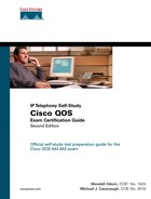
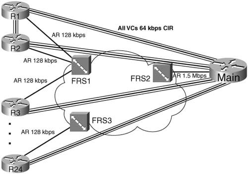
Policing can be useful in multiaccess WANs (Frame Relay and ATM networks) for the same reason that it was useful for the ISP connection described earlier. Whenever data can be sent faster than the contracted rate, the danger exists that a network will be overrun when many sites exceed their contract at the same time. An example will help you understand a few of the issues. Figure 6-2, the network diagram for PB Tents network, has been expanded to show 12 branches, with a single central site.

Each branch can send traffic at 128 kbps, but each branch only has a contracted 64-kbps CIR on their respective VCs to the main site. If all 12 sites conform to their CIRs, the Frame Relay network should be able to handle the load. If all 12 sites offer 128 kbps of traffic for long periods, however, the provider may still go ahead and try to forward all the traffic, because most Frame Relay providers overbuild their core networks. They also like to imply in their sales pitch that the customer gets to send excess packets for free.
Of course, at some point, if every customer of this provider sent traffic at full line rates for a period of time, the network would probably congest. The same options exist for the Frame Relay network as for an ISP — not to police but build more capacity; police to CIR, and deal with the sales and customer satisfaction issues; or police at something over CIR, and deal with the sales and customer satisfaction issues in slightly different ways.
To police the network in Figure 6-2, the Frame Relay switches can be configured to perform the policing, or the routers can be used. Traditionally, policing is performed as packets enter a network, which would suggest policing as packets enter the Frame Relay switches from the customer. If the service provider actually controls the edge routers in the enterprise network, however, the policing feature can be performed as packets exit the routers, going toward the Frame Relay cloud. If the customer controls the routers at the edge of the cloud, policing in these routers may be risky for the service provider, just because of the possibility that some customers might turn off policing to get more capacity for free.
The Cisco QoS exam covers policing in IOS routers using CB Policing. The exam does not cover policing in Frame Relay switches, or in LAN switches, although the basic concepts are the same.
Networks use traffic shaping for two main reasons:
![]() To shape the traffic at the same rate as policing (if the service provider polices traffic)
To shape the traffic at the same rate as policing (if the service provider polices traffic)
![]() To avoid the effects of egress blocking
To avoid the effects of egress blocking
For instance, consider Branches 1 and 24 in Figure 6-3. Branch 1 does not shape, whereas Branch 24 does shape to 96 kbps. In both cases, the Frame Relay switches they are configured to police packets at a 96-kbps rate. (The CIR in each case is 64 kbps. Therefore, the service provider is not policing aggressively. The PB Tents engineer wants to get as much bandwidth as possible out of the service, so he shapes at 96 kbps rather than the 64-kbps CIR.)
For Branch 1, the absence of shaping ensures that R1 will not artificially delay any packets. However, the policing performed at FRS1 will discard some packets when R1 sends more than 96-kbps worth of traffic. Therefore, some packets will be dropped, although the packets that are not dropped will not experience extra shaping delay. This strategy makes sense when the traffic from Branch 1 is not drop sensitive, but may be delay and jitter sensitive.
For Branch 24, the presence of shaping ensures that R1 will artificially delay some packets. However, the policing performed at FRS3 will not discard packets, because R1 will not send more than 96-kbps worth of traffic. Therefore, no packets will be dropped, although some packets will experience more delay and jitter. This strategy makes sense when the traffic from Branch 24 is drop sensitive, but not delay and jitter sensitive.
The other reason to use shaping is to avoid the effects of egress blocking. Egress blocking occurs when packets try to exit a multiaccess WAN, such as Frame Relay and ATM, and cannot exit the network because of congestion. Automobile traffic patterns cause the same kinds of behavior as egress blocking. In the morning, for instance, everyone in the state may try to commute to the same small, downtown area of a big city. Even though an eight-lane highway leads into the city, it may seem that everyone living in the surrounding little towns tries to get off at the few exits of the highway between 7 and 8 a.m. each morning. The highway and exits in the downtown area become congested. Similarly, in the afternoon, if everyone tries to reach the suburbs through one exit off the highway at 5:30 p.m., the eight-lane highway feeding into the two-lane exit road becomes congested. Likewise, although plenty of capacity may exist in a network, egress blocking can occur for packets trying to exit the network.
Figure 6-4 illustrates what happens with egress blocking, using a Frame Relay network as an example.

Suppose that all 24 branches shape at 64 kbps. The cumulative traffic sent by the branches to the main site is 1.5 Mbps, if each branch simultaneously sends 64 kbps. Because the Main router has a T/1 installed, FRS2 should not experience congestion when forwarding packets out of the access link to the Main router. However, what if shaping were not used at the branches? If all 24 branches were to send traffic at 128 kbps (access rate) for a period of time, the cumulative offered load would be about 3 Mbps. Packets would begin to queue trying to exit FRS2’s interface connected to the Main router. The packets would experience more delay, more jitter, and eventually more packet drops as the FRS2 output queue filled. Notice that the service provider did not do any policing—egress blocking still occurred, because the branches could collectively overload the egress link between the cloud and the main site.
Interestingly, even if policing were used, and shaping at the branches, egress blocking could still occur. In Figure 6-3, shaping and policing were configured at 96 kbps, because the service provider did not want to be too aggressive in enforcing the traffic contract. With all 24 branches sending 96 kbps at the same time, about 2.25 Mbps of traffic needs to exit FRS2 to get to the Main router. Again, egress blocking can occur, even with policing and shaping enabled!
Similarly, egress blocking can occur right to left in the figure as well. Imagine that the Main router receives 11 consecutive 1500-byte packets from a LAN interface, destined to Branch 24. It takes the Main router roughly 100 milliseconds to send the packets into the Frame Relay network, because its access link is a T/1. When the frames arrive in FRS1, they need to be sent out the access link to R24. However, this access link runs at 128 kbps. To send these 11 packets, it takes slightly more than 1 second just to serialize the packets over the link! Most of the packets then wait in the output queue on FRS3, waiting their turn to be sent. This simple case is another example of egress blocking, sometimes just referred to as a speed mismatch.
One solution to the egress blocking problem is to shape the traffic. In the example network, shaping all VCs at the branches to 64 kbps would ensure that the cumulative offered load did not exceed the access rate at the main site. Similarly, if the Main router shaped the VC to R1 to 64 kbps, or even 128 kbps, the egress blocking problem on FRS1 would be solved.
In both cases, however, delay and jitter occurs as a result of the shaping function. Instead of having more queuing delay in the Frame Relay switches, shaping delays occur in the router, because packets wait in router shaping queues. With the queuing occurring in the routers, however, the features of IOS queuing tools can be used to better manipulate the traffic, and give better delay characteristics to delay-sensitive traffic. For instance, with the shaping queues forming in a router, the router can use Low Latency Queuing (LLQ) to dequeue Voice over IP (VoIP) packets first. A Frame Relay switch cannot perform complicated queuing, because the Frame Relay switch does not examine fields outside the Frame Relay or IP header when making forwarding and queuing decisions.
Table 6-2 summarizes some of the key points about the rationale behind when you should use policing and shaping.

Shaping only makes sense when the physical clock rate of a transmission medium exceeds a traffic contract. The most typical case for shaping involves a router connected to a Frame Relay or ATM network. More often today, however, connections to ISPs use a point-to-point serial link or an Ethernet link between an enterprise and the ISP, with a traffic contract defining lower traffic volumes than the physical link.
Routers can only send bits out an interface at the physical clock rate. To have the average bit rate, over time, be lower than the clock rate, the router just has to send some packets for some specified time period, and then not send any packets for another time period. To average sending at a packet rate of half the physical link speed, the router should send packets half of the time, and not send the other half of the time. To make the average rate equal to 1/4 of the physical link speed, the router should send 1/4 of the time, and not send packets 3/4 of the time. Over time, it looks like a staccato series of sending, and silence.
You can understand traffic-shaping logic by reviewing just a few simple examples. Of course, you need to know a few more details for the exam! However, the basics follow these simple examples: If R1 has a 128-kbps access rate, and a 64-kbps CIR, and the engineer wants to shape the traffic to match CIR (64 kbps), R1 just has to send traffic on the link half of the time. If, over time, R1 sends traffic half of the time, at 128 kbps (because that’s the only rate it can actually send traffic), the average over that time is 64 kbps. The concept is that simple!
A few more simple examples here emphasize the point. Referring to Figure 6-4, assume R1 wants to shape at 96 kbps, because the Frame Relay switch is policing at 96 kbps. With a 128-kbps access rate, to shape to 96 kbps, R1 should send 3/4 of the time, because 96/128 = 3/4.
Again from Figure 6-4, if the Main router wants to shape the VC connecting it to R24 at 128 kbps, to avoid the egress-blocking problem, the Main router needs to send packets 128/1536 (actual available bit rate for T/1 is 1.536 Mbps), or 1/12 of the time. If the Main router wants to shape that same VC to 64 kbps, to match the CIR, the Main router should send packets over that VC at 64/1536, or 1/24, of the time.
Traffic shaping implements this basic logic by defining a measurement interval, and a number of bits that can be sent in that interval, so that the overall shaped rate is not exceeded. Examples help, but first, Table 6-3 lists some definitions.

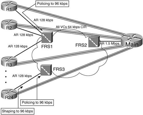
The actual processes used by traffic shaping, and the terms in Table 6-3, will make much more sense to you with a few examples. The first example, as outlined in Figure 6-5, shows the familiar case where R1 shapes to 64 kbps, with a 128-kbps access link.
The router should send literally half of the time to average sending 64 kbps on a 128-kbps link. Traffic shaping accomplishes this by sending up to half of the time in each Tc.
As shown in the figure, R1 sends at line rate for 62.5 ms, and then is silent for 62.5 ms, completing the first interval. (The Tc defaults to 125 ms for many shaping tools; CB Shaping happens to default to another Tc in this case, but the concept is still valid.) As long as packets are queued and available, R1 repeats the process during each interval. At the end of 1 second, for instance, R1 would have been sending for 62.5 ms in 8 intervals, or 500 ms—which is .5 seconds. By sending for half of the second at 128 kbps, R1 will have sent traffic at an average rate of 64 kbps.
IOS traffic shaping does not actually start a timer for 62.5 ms, and then stop sending when the timer stops. IOS actually calculates, based on the configuration, how many bits could be sent in each interval so that the shaped rate would be met. This value is called the committed burst (Bc) for each interval. It is considered a burst, because the bits actually flow at the physical line rate. The burst is committed, because if you send this much every interval, you are still conforming to the traffic contract. In this example, the Bc value is set to 8000 bits, and the actual process allows the shaper to send packets in each interval until 8000 bits have been sent. At that point, the shaper waits until the Tc has ended, and another interval starts, with another Bc worth of bits sent in the next interval. With an interval of 125 ms, and 8000 bits per interval, a 64-kbps shaped rate is achieved.
The Bc value is calculated using the following formulas:
![]()
or
![]()
In the first formula, which is scattered throughout the Cisco documentation, the formula assumes that you want to shape at the CIR. In some cases, however, you want to shape to some other rate, so the second formula gives the more exact formula. For instance, if a Shaping tool had a default of 125 ms for Tc, and with a shaped rate of 64 kbps, the Bc would be
![]()
When configuring shaping, you typically configure the shaping rate and optionally the Bc. If you configure both values, IOS changes the Tc so that the formula is met; you never actually configure the value of Tc. If you just configure the shaping rate, depending on the Shaping tools, IOS assumes a particular value for Tc or Bc, and then calculates the other value.
The section covering CB Shaping later in this chapter covers how CB Shaping calculates Tc and Bc assuming that only the shaping rate has been configured. However, if you configure both the shaping rate and the Bc, IOS calculates Tc as follows:
![]()
or
![]()
Again, the formula referring to CIR assumes that you shape to the CIR value, whereas the second formula refers to the shaping rate, because you can configure shaping to shape at a rate different from CIR.
Additional examples should bring the concepts together. Previously you read the example of the PB Tents company shaping at 96 kbps over a link using a 128-kbps clock rate, because the Frame Relay provider policed at 96 kbps. If the shaping function is configured with a shaping rate of 96 kbps, assuming a Tc of 125 ms, the formulas specify the following:
![]()
Figure 6-6 shows what happens in this example. For each interval, shaping can release 12,000 bits, which takes 93.75 ms. 93.75/125 = 3/4, implying that the router will average sending bits at 3/4 of the clock rate, or 96 kbps.

Traffic shaping uses the idea of a number of bits per interval for implementation because it’s much more efficient than calculating rates all the time. The shaper just grabs the next packet, decrements the Bc values by the number of bits in the packet, and keeps doing that until the Bc value is consumed. At that point, shaping waits until the Tc has expired, when shaping gets to send another Bc worth of bits.
The length of Tc may have some impact on the delay and jitter characteristics of the packets being shaped. Consider another example, with the Main router sending packets to R24, shaping at 128 kbps, but with a T/1 access link. Figure 6-7 shows the shaping details.

Simply put, at T/1 speeds, it does not take long to send the Bc worth of bits per interval. However, The Tc value of 125ms may be a poor choice for delay-sensitive traffic. Suppose that a VoIP packet arrives at Main, and it needs to be sent to R24. Main uses LLQ, and classifies VoIP into the low-latency queue, so the new VoIP packet will be sent next. That’s true—unfortunately, the packet sent just prior to the new VoIP packet’s arrival consumed all of Bc for this Tc. How long does the VoIP packet have to wait before the current Tc will end and a new one will begin? Well, it only took 10 ms to send the Bc worth of bits, so another 115 ms must pass before the current Tc ends, and the VoIP packet can be sent! With one-way delay budgets of 150 to 200 ms, a single shaping delay of 115 ms just will not work. Therefore, Cisco recommends that when you have delay-sensitive traffic, configure Bc such that Tc is 10 ms or less. In this same example, if the Bc were configured to 1280 bits, Tc = 1280/128,000 = .010 seconds, or 10 ms.
Note Many of you might be concerned about the relatively small Bc of 1280 bits, or only 160 bytes! Most packets exceed that length. Well, as it turns out, you will also typically use fragmentation in the exact same cases. To accommodate the same delay-sensitive traffic, the fragments will be of similar size—in fact, as you will read in Chapter 8, “Link Efficiency Tools,” the fragmentation size will likely be 160 bytes in this particular example. Therefore, with delay-sensitive traffic, you will drive Tc down to about 10 ms by lowering Bc, and the Bc value will essentially allow a single fragment per Tc. By doing so, you reduce the shaping delay waiting on the next Tc to occur, and you reduce the serialization delay by fragmenting packets to smaller sizes.
The next several sections continue the discussion of how traffic shaping works, covering excess burst, queuing, adaption, and some concepts about enabling shaping.
Traffic shaping includes the capability to send more than Bc in some intervals. The idea is simple: Data traffic is bursty, so after a period of inactivity, it would be nice if you could send more than Bc in the first interval after traffic occurs again. This extra number of bits is called the burst excess, or Be. Traffic-shaping tools allow Be as an option.
The underlying operation of traffic shaping to allow for Be requires a little more insight into how traffic shaping works, and it also requires us to understand the concept of token buckets. Token buckets can be used to describe how shaping and policing are implemented.
Ignoring Be for a moment, imagine a bucket filled with tokens, like subway tokens. In the token-bucket scenario, each token lets you buy the right to send 1 bit. One token bucket is used for formal operation of traffic shaping as discussed earlier; this bucket has a size of Bc.
Two main actions revolve around the token bucket and the tokens:
![]() The re-filling of the bucket with new tokens
The re-filling of the bucket with new tokens
![]() The consumption of tokens by the Shaper to gain the right to forward packets
The consumption of tokens by the Shaper to gain the right to forward packets
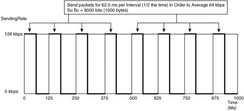
For filling the token bucket, the bucket is filled to its maximum capacity, but no more, at the beginning of each Tc (assuming that Be = 0 for the time being). Another way you can think of it as if the Shaper dumps Bc worth of tokens into the bucket at the beginning of every interval; however, if there’s not enough room in the bucket, because not all the tokens were used during the previous time interval, some tokens spill out. Those spilled tokens can’t be used. The net result, either way you look at it, is that the interval starts with a full token bucket of size Bc. Figure 6-8 shows the basic idea:
Every time a packet is sent, traffic shaping spends tokens from the token bucket to buy the right to send the packet. If the packet is 1000 bits long, 1000 tokens are removed from the bucket. When traffic shaping tries to send a packet, and the bucket does not have enough tokens in it to buy the right to send the packet, traffic shaping must wait until the next interval, when the token bucket is refilled.
An analogy of token bucket is a child and the allowance the child receives every Saturday morning. For the sake of argument, assume the weekly allowance is $10. The child may spend the money every week; if the child doesn’t spend it, he may save up to buy something more expensive. Imagine that the child’s parents are looking at the child’s piggybank every Saturday morning, however, and if they find some leftover money, they just add a little more money so that the child always starts Saturday morning with $10! After a few weeks of this practice, the child would likely try to spend all the money each week, knowing that he would never be able to save any more than $10. Similarly, the Bc of bits, or the tokens in the bucket if you prefer, are only usable in that individual Tc interval, and the next Tc (interval) always starts with Bc tokens in the bucket, but never any more.
Traffic shaping implements Be by making the bucket bigger. In fact, to support an excess burst, the bucket now contains Bc plus Be worth of tokens. The filling of tokens into the bucket at the beginning of each interval, and the draining of tokens to gain the right to send packets, remains the same. For instance, at the beginning of each interval, the Shaper still tries to fill the bucket with Bc tokens. If some spill out, because there’s no more room for more tokens in the bucket, those tokens are wasted.
The key advantage gained by having Be—in other words, having a token bucket of size Bc plus Be—is that the token bucket is larger. As a result, after some time during which the actual bit rate is lower than the shaping rate, the token bucket fills with tokens. If in the next interval more than Bc bits needed to be sent, the Shaper could send them—up to the number of tokens in the bucket, namely Bc + Be. Basically, the Shaper allows the amount of data passed by the shaper to burst.
Figure 6-9 shows a graph of how shaping works when using Be. The shaper represented by the graph shapes to a CIR of 64 kbps, over a 128-kbps link. The Bc has been set to 8000 bits, with an additional 8000 bits for Be.

The example in Figure 6-9 assumes that enough inactive or slow periods have occurred, just prior to this example, so that the token bucket is full. In other words, the token bucket holds Bc + Be tokens, which is 16,000 tokens in this example. A large amount of traffic shows up, so traffic shaping sends as fast as it can until it runs out of tokens.
In the first interval, traffic shaping can send a total of 16,000 bits. On a 128-kbps link, assuming a 125-ms Tc, all 125 ms are required to send 16,000 bits! Effectively, in this particular case, after a period of inactivity, R1 sends continuously for the entire first interval.
To begin the second interval, Shaping adds Bc (8000) tokens to the bucket. Those tokens do not fill the bucket, but it does allow the shaper to pass 8000 bits, which requires half the time interval. So, in this example, the shaper will send for 187.5 ms (the entirety of the first 125 ms interval, plus half of the second interval) until traffic shaping artificially slows down the traffic. Thus, the goal of allowing a burst of data traffic to get started quickly is accomplished with Be.
The rate at which the shaping function shapes traffic can vary over time. The adaption or adaptation process causes the shaper to recognize congestion and reduce the shaping rate temporarily, to help reduce congestion. Similarly, adaption notices when the congestion abates and returns the shaping rate to the original rate.
Two features define how adaption works. First, the shaper must somehow notice when congestion occurs, and when it does not occur. Second, the shaper must adjust its rate downward and upward as the congestion occurs and abates.
Figure 6-10 represents three different ways in which the main router can notice congestion. Three separate lines represent three separate frames sent to the main router, signifying congestion. Two of the frames are data frames with the Frame Relay backward explicit congestion notification (BECN) bit set. This bit can be set inside any Frame Relay frame header, signifying whether congestion has occurred in the direction opposite to the direction of the frame with the bit set. The third (bottom) message is a Foresight message. Stratacom, and later Cisco after they acquired Stratacom, defined Foresight as a signaling protocol in Frame Relay and ATM networks, used to signal information about the network, such as congestion information. If the Frame Relay network consists of Cisco/ Stratacom WAN switches, the switch can send Foresight messages, and Cisco routers can react to those messages. Following the figure, each of the three variations for the Main router to recognize that congestion is occurring is explained in detail.
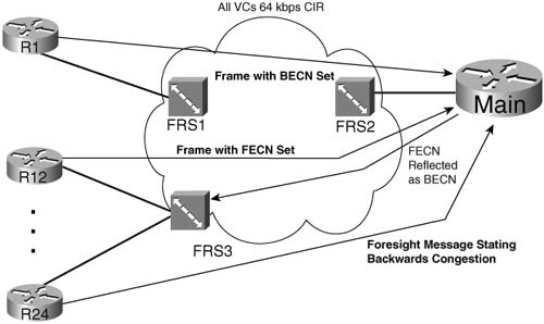
First consider the BECN frame. Backward means that the congestion exists in the opposite, or backward, direction, as compared with the direction of the frame. Therefore, if FRS1 notices congestion trying to send frames to R1 (right to left in the figure), on the next frame sent by R1 (left to right in the figure), FRS1 can mark the BECN bit. In fact, any device can set the forward explicit congestion notification (FECN) and BECN bits—however, in some networks, the Frame Relay switches do set the bits, and in some, they do not.
If the BECN bit is set, the Main router, if using adaptive shaping, reduces its shaping rate on the VC to R1. Because the congestion occurs right to left, as signaled by a BECN flowing left to right, router Main knows it can slow down and help reduce the congestion. If Main receives another frame with BECN set, Main slows down more. Eventually, Main slows down the shaping rate until it reaches a minimum rate, sometimes called the minimum information rate (MIR), and other times called the mincir.
Similarly, if Main receives a Frame from R12 with FECN set, the congestion is occurring left to right. It does not help for Main to slow down, but it does help for R12 to slow down. Therefore, the Main router can “reflect” the FECN, by marking the BECN bit in the next frame it sends on the VC to R12. R12, receiving a BECN, can reduce the shaping rate.
Finally, Foresight messages are separate, nondata signaling frames. Therefore, when the congestion occurs, Foresight does not need to wait on a data frame to signal congestion. In addition, Foresight sends messages toward the device that needs to slow down. For instance, a switch notices congestion right to left on the VC between Main and R24. The switch generates and sends a Foresight message to Main, using that same VC, so Main knows it needs to slow down its shaping rate on that VC temporarily. When configuring adaptive shaping, you configure the minimum and maximum shaping rate. With no congestion, CB Shaping uses the maximum rate. When the Shaper receives a BECN or Foresight message, it slows down by 25 percent of the maximum rate. In order to slow down, CB Shaping actually simply decreases Bc and Be by 25%, keeping the Tc value the same. In other words, CB Shaping allows fewer bits to pass in each time interval. If the Shaper continues to receive BECNs, the Shaper continues to slow down by 25 percent of the maximum rate per Tc , until the minimum rate is reached.
The rate grows again after 16 consecutive intervals occur without a BECN or Foresight congestion message. The shaping rate grows by 1/16 of the maximum rate during each Tc, until the maximum rate is reached again. To do that, the formerly-reduced Bc and Be values are increased by 1/16 oftheir configured values each Tc. Because of that, the formula for calculating how much CB Shaping increases the rate per time interval as actually showing the increase in BC and Be values. The formula for the amount of increase per interval is:
![]()
Shaping can be applied to the physical interface, a subinterface, or in some cases, to an individual VC. Depending on the choice, the configuration causes traffic shaping to occur separately for each VC, or it shapes several VCs together. In most cases, engineers want to shape each VC individually.
When shaping is applied to an interface for which VCs do not exist, shaping is applied to the main interface, because there are no subinterfaces or VCs on those interfaces. On Frame Relay and ATM interfaces, however, some sites have multiple VCs terminating in them, which means that subinterfaces will most likely be used. In some cases, more than one VC is associated with a single multipoint subinterface; in other cases, point-to-point subinterfaces are used, with a single VC associated with the subinterface. The question becomes this: To shape per VC, where do you enable traffic shaping?
First, consider a typical branch office, such as R24 in Figure 6-11. R24 has a single VC to the Main site at PB Tents. Because R24 only has the single VC, the configuration on R24 may not even use subinterfaces at all. If the configuration does not use subinterfaces on R24’s serial link, traffic shaping can be configured on the physical interface. If the configuration includes a subinterface, you can enable traffic shaping on the physical interface, or on the subinterface. Because there is only one VC, it does not really matter whether shaping is enabled on the physical interface, or the subinterface—the behavior is the same.
Now consider the Main router. It has a VC to each remote site. (Also notice that a VC has been added between R1 and R2, just to make things interesting.) So, on the main router, point-to-point subinterfaces are used for the VCs to branches 3 through 24, and a multipoint subinterface is used for the two VCs to R1 and R2. To shape each VC to branches 3 through 24 separately, shaping can be configured on the subinterface. However, shaping applied to a multipoint subinterface shapes all the traffic on all VCs associated with the subinterface. To perform shaping on each VC, you need to enable shaping on each individual data-link connection identifier (DLCI).
As it turns out, CB Shaping can be applied per subinterface, but not per-VC on multipoint subinterfaces. In the example in Figure 6-11, CB Shaping could shape all traffic from router Main to both R1 and R2, but it could not shape traffic to R1 separately from the traffic going to R2.
In summary, most QoS policies call for shaping on each VC. The configuration commands used to enable shaping differ slightly based on the number of VCs, and how they are configured. Table 6-4 summarizes the options.

Shaping tools support a variety of queuing tools that can be applied to the packets waiting in the shaping queue(s). At the same time, IOS supports queuing tools for the interface software queue(s) associated with the physical interface. Deciding when to use queuing tools on shaping queues, when to use them on the interface software queues, and how the configurations differ in each case, can be a little confusing. This section attempts to clear up some of that confusion.
Note The current QoS exam does not cover any details about the other Shaping tools besides CB Shaping. However, the idea of how to use Queuing tools for Shaping, and to also use Queuing tools for the interface software queues, confuses many people. The rest of the details in this short section on “Queuing and Traffic Shaping” discuss those details. This material is probably outside what you’ll see on the exam, but is important enough to include coverage.
To begin, Table 6-5 lists the traffic-shaping tools, and the queuing tools supported by each for the shaping queues.

When a Shaper uses a queuing tool, instead of creating a single FIFO shaping queue, it creates multiple shaping queues based on the Queuing tool. For instance, if FRTS were configured to use Priority Queuing (PQ) for the shaping queues, it would create four queues for shaping, named High, Medium, Normal, and Low. Figure 6-12 shows the basic idea, with shaping enabled on the physical interface, FIFO Queuing on the physical interface, and PQ configured for shaping the only VC.

The shaping queues exist separately from the interface software queues, as seen in Figure 6-12. With PQ applied to the Shaper, four shaping queues exist for this VC. When the Shaper decides to allow another packet to be sent, it takes the next packet from the PQ shaping queues, according to PQ scheduler logic. Those packets are placed into software queues associated with the physical interface and then forwarded out the interface—in this case shown as a single FIFO queue.
In some cases, the shaping queues are bypassed, and in other cases, the interface software queues are bypassed. To understand why, consider Figure 6-13, which demonstrates part of the logic behind the decision for determining when each queue should be used.
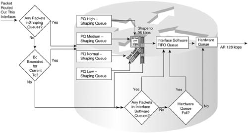
Packets are held in a shaping queue or interface output queue only if there is some reason why the packet must wait to take the next step. For instance, you already know that if the Hardware Queue is not full, packets are immediately placed into the Hardware Queue, bypassing the interface Software Queue. Likewise, if shaping decides that a packet does not need to be delayed, because the shaping rate has not been exceeded, it can go directly to the interface output queue, or even to the Hardware Queue.
Many QoS designs call for shaping per VC, as mentioned in the preceding section. Suppose that a router has two 64-kbps CIR VCs sharing an access link, each configured on a separate point-to-point subinterface. Shaping queues will be created for each VC. A single set of interface output queues will be created, too. Figure 6-14 depicts the overall idea.
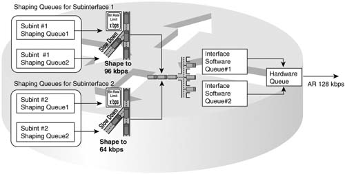
The shaping tool creates a set of queues for each subinterface or VC, based on the queuing tool configured for use by the shaper. IOS creates only one set of interface software queues for the physical interface, based on the queuing configuration on the physical interface, as covered in Chapter 5, “Congestion Management.” In Figure 6-14, two sets of shaping queues have been created, one per VC. Both VCs feed the single set of interface output queues.
Finally, in this particular example, congestion can occur at the physical interface. The total of the two shaping rates listed in Figure 6-14 is 160 kbps, which exceeds the access rate (128 kbps). Because interface output queues can fill, it helps to apply a queuing tool to the interface output queues in this case.
Policers, like Shapers, need to determine whether a packet is within the traffic contract. To do so, it performs a metering process to effectively measure the cumulative byte-rate of the arriving packets. Based on that metering process, the policer acts on the packet as follows:
![]() Allowed to pass
Allowed to pass
![]() Dropped
Dropped
![]() Re-marked with a different IP precedence or IP DSCP value.
Re-marked with a different IP precedence or IP DSCP value.
Policers can be a little more complicated than Shapers. Like CB Shaping, CB Policing uses token buckets for the mechanics of how to monitor traffic and decide which packets are outside the traffic contract. If you want CB Policing to decide if a packet either confirms to or exceeds the contract, it will use a single token bucket, like CB Shaping. You can think of this style of policing as having two classes, as determined by the metering process. The two categories are conforming and exceeding.
However, CB Policing can be configured to use three categories about whether a packet is conforming to the contract:
![]() Conforming—Packet is inside the contract
Conforming—Packet is inside the contract
![]() Exceeding—Packet is using up a excess burst capability
Exceeding—Packet is using up a excess burst capability
![]() Violating—Packet is totally outside the contract
Violating—Packet is totally outside the contract
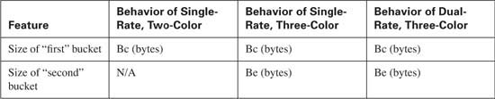
When configuring CB Policing, you can choose to define with the conforming and exceeding actions, or you can choose to configure all three actions. If you use only two categories, the policer is sometimes called a “two-color” policer, and it uses a single token bucket. If you configure all three categories, CB Policing uses dual token buckets, and is called a “three-color” policer. (The ideas behind the three-color policing function are described further in RFC 2697, “A Single-rate Three Color Marker”.)
CB Policing also allows the concept of a dual-rate policer, which means that the policer actually monitors two different rates, called the Committed Information Rate (CIR) and the Peak Information Rate (PIR). To do that, CB Policing must use another twist on the logic of how the two token buckets are used. This more advanced style of policing allows a router to enforce traffic contracts for two sustained rates, which gives service providers a lot more flexibility in terms of what they offer to their customers. This concept of policing and monitoring two rates is defined in RFC 2698, “A Dual-rate Three-Color Marker”.
The sections that follow cover, in order, single rate, single bucket (two-color) CB Policing; single rate policing, but with two token buckets (three-color); and finally the RFC 2698 concept of a two-rate, three-color policer, meaning two token buckets, and two separate policing rates.
When using token buckets for policing, two important things happen. First, tokens are replenished into the bucket. Later, when the policer wants to decide if a packet conforms to the contract or not, the policer will look into the bucket, and try to get enough tokens to allow the packet through. If there’s enough, the policer will “spend” the tokens, removing them from the bucket, in order to have the right to allow the packet past the policer.
With Policing, think of each token as the right to send a single byte; with Shaping, each token represented a bit. First, consider how CB Policing fills the single token bucket. Unlike CB Shaping, CB policing replenishes tokens in the bucket in response to a packet arriving at the policing function, as opposed to using a regular time interval (Tc). Every time a packet is policed, CB policing puts some tokens back into the Bucket. The number of tokens placed into the Bucket is calculated as follows:
![]()
Note that the arrival times’ units are in seconds, and the police rate is in bits per second, with the result being a number of tokens. Each token represents the right to send 1 byte, so the formula includes the division by 8 in order to convert the units to bytes instead of bits.
The idea behind the formula is simple — essentially, a small number of tokens are replenished before each packet is policed, with an end result of having tokens replenished at the policing rate. Suppose, for instance, that the police rate is 128,000 bps (which happens to equal 16,000 bytes per second.) If 1 second has elapsed since the previous packet arrived, CB Policing would replenish the bucket with 16,000 tokens. If 0.1 seconds had passed since the previous packet had arrived, CB Policing would replenish the bucket with 0.1 seconds worth of tokens, or 1600 tokens. If .01 seconds had passed, CB Policing would replenish 160 tokens at that time. Essentially, the Bucket is replenished with a prorated number of tokens based on how long ago it was last replenished.
The second part of using a bucket relates to the policer’s choice as to whether a packet conforms to the contract or not. CB Policing compares the number of bytes in the packet to the number of tokens the token bucket. CB policing’s decision is simple, as noted here:
![]() If the number of bytes in the packet is less than or equal to (<=) the number of tokens in the bucket, the packet conforms. CB policing removes tokens from the bucket equal to the number of bytes in the packet, and performs the action for packets that conform to the contract.
If the number of bytes in the packet is less than or equal to (<=) the number of tokens in the bucket, the packet conforms. CB policing removes tokens from the bucket equal to the number of bytes in the packet, and performs the action for packets that conform to the contract.
![]() If the number of bytes in the packet is greater than (>) the number of tokens in the bucket, the packet exceeds the contract. CB policing does not remove tokens from the bucket, and performs the action for packets that exceed the contract.
If the number of bytes in the packet is greater than (>) the number of tokens in the bucket, the packet exceeds the contract. CB policing does not remove tokens from the bucket, and performs the action for packets that exceed the contract.
Therefore, the logic used by a single-rate, two-color policer is simple. The bucket gets replenished with tokens based on packet arrival time. If the packet conforms, CB Policing either forwards, discards, or re-marks the packet, and some tokens are then removed from the bucket. If the packet exceeds, CB Policing either forwards, discards, or re-marks the packet, but no tokens are removed from the bucket. (Note that discarding packets that conform is a valid configuration option, but it is not particularly useful.)
When you want the policer to support both a committed burst (Bc) and an excess burst (Be), the policer uses two token buckets. By using two token Buckets, CB Policing can categorize packets into three groups:
![]() Conform
Conform
![]() Exceed
Exceed
![]() Violate
Violate
The intent of these three categories is to allow the policer to decide if packets totally conform, whether they are using the excess burst capability (exceed), or whether the packet puts the data beyond even the excess burst (violate).
Note There is no official name for the two token buckets, so I will refer to them simply as the Bc bucket and the Be bucket in this section.
Just like with a single token bucket, to understand how CB Policing works with two buckets is to understand how the buckets are filled and drained. CB Policing continues to replenish the Bc bucket when a packet arrives. However, any spilled tokens when filling the Bc bucket are not simply wasted. If the Bc bucket is full, the extra, or spilled tokens, replenish the Be bucket. If the Be bucket fills, the excess tokens spill out and are wasted. Figure 6-15 shows the basic process:

With Bc and Be configured, CB policing uses dual token buckets, and the algorithm is simple:
1. If the number of bytes in the packet is less than or equal to (<=) the number of tokens in the Bc Bucket, the packet conforms. CB policing removes tokens from the Bc Bucket equal to the number of bytes in the packet, and performs the action for packets that conform to the contract.
2. If the packet does not conform, and the number of bytes in the packet is less than or equal to (<=) the number of tokens in the Be Bucket, the packet exceeds. CB policing removes tokens from the Be Bucket equal to the number of bytes in the packet, and performs the action for packets that exceed the contract.
3. If the packet neither conforms nor exceeds, it violates the traffic contract. CB policing does not remove tokens from either bucket, and performs the action for packets that violate the contract.
Essentially, packets that fit within Bc conform, those that require the extra bytes allowed by Be exceed, and those that go beyond even Be are considered to violate the traffic contract.
Dual Token Bucket CB Policing with a single rate provides a very useful function. After a period of low activity, a larger burst of data can be considered to either conform to or exceed the traffic contract, without violating the traffic contract. Because data tends to be bursty, the idea of a policer with bursting capability makes a lot of sense.
Dual Token Bucket with Dual-rate policing also provides a bursting feature, but with dual-rate, the CB Policer allows you to essentially set two different sustained rates. Packets that fall under the lower rate—the Committed Information Rate (CIR)—conform to the traffic contract. A second sustained rate—the Peak Information Rate (PIR)—defines a traffic rate above CIR. Packets that happen to exceed the CIR, but fall below PIR, are considered to exceed the contract, but not to violate it. Finally, packets beyond even the PIR are considered to violate the contract.
As usual, the mechanics of how it all works behind the scenes relates to how the policer replenishes tokens into the buckets, and how the policer then takes tokens from the buckets during the process of deciding if a packet conforms, exceeds, or violates the traffic contract. First, consider Figure 6-16, which shows the refill process works for the two buckets. In this case, the buckets are referred to as the CIR bucket and the PIR bucket, respectively.

A couple of differences exist between the token refilling process of the single rate, three-color policing of the previous section. First, note that both buckets are filled upon the arrival of a packet that needs to be policed. However, the PIR bucket is refilled with tokens directly, instead of having to rely on spillage from the refilling of the CIR bucket. Essentially, this means that the PIR bucket does not have to rely on a period of low or no activity in order to get more tokens. Also note that when refilling, any tokens that spill from either bucket are wasted.
The refilling of the two buckets based on two different rates is very important. For example, imagine you set a CIR of 128 kbps (16 kilobytes/second), and a PIR of 256 kbps (32 kilobytes/second). If .1 seconds passed before the next packet arrived, then the CIR bucket would be replenished with 1.6 kilobytes of tokens (1/10 of 1 seconds worth of tokens, in bytes), while the PIR bucket would be replenished with 3.2 kilobytes of tokens. So, there are more tokens to use in the PIR bucket, as compared to the CIR bucket.
As usual, the second part of the process involves how the policer thinks about the tokens in the buckets in order to decide if the packet conforms, exceeds, or violates the traffic contract. The logic is similar to the single rate, two bucket policing described earlier, but with a twist for what happens for conforming packets:
1. If the number of bytes in the packet is less than or equal to (<=) the number of tokens in the CIR bucket, the packet conforms. CB Policing removes tokens from the CIR equal to the number of bytes in the packet, and performs the action for packets that conform to the contract. CB Policing also removes the same number of tokens from the PIR bucket.
2. If the packet does not conform, and the number of bytes in the packet is less than or equal to (<=) the number of tokens in the PIR bucket, the packet exceeds. CB Policing removes tokens from the PIR bucket equal to the number of bytes in the packet, and performs the action for packets that exceed the contract.
3. If the packet neither conforms nor exceeds, it violates the traffic contract. CB Policing does not remove tokens from either bucket, and performs the action for packets that violate the contract.
Even before you read this list, you probably guessed the base logic. If there are enough tokens in the CIR bucket, the packet conforms; if not, and there’s enough in the PIR bucket, it exceeds; if not, the packet violates the contract. The new part revolves around the fact that even if the packet conforms, the policer takes tokens from the PIR bucket.
An example can help. Imagine that CB Policing has been configured for the following:
![]() CIR 128 kbps (16 kilobytes/second)
CIR 128 kbps (16 kilobytes/second)
![]() Bc of 8000 bytes
Bc of 8000 bytes
![]() PIR of 256 kbps (32K kilobytes/second)
PIR of 256 kbps (32K kilobytes/second)
![]() Be of 16,000 bytes
Be of 16,000 bytes
Effectively, PIR and Be are double the values of CIR and Bc. Now imagine that both buckets are full of tokens, and a bunch of packets arrive at the same instant. Because they arrive at the same instant, the replenishment of tokens into the buckets is either 0, or negligible—so for the sake of discussion, assume no new tokens are added to either bucket during this example.
The first 8000 bytes worth of packets pass through the policer, with the packets considered to conform. The CIR bucket is decremented to 0. At the same time, the PIR bucket is also decremented, from 16,000 to 8,000 tokens.
For the next 8000 bytes of packets, the policer decides that the packets exceed the contract, and the policer removes tokens from the PIR bucket. Finally, after the rest of the packets are considered to violate the traffic contract, at least until some time passes, allowing more tokens to be added to the two buckets.
CB Policing includes a lot of small details about how it chooses which packets conform to, exceed, or violate a traffic contract. To help with exam prep, Table 6-6 lists the key points about how CB Policing uses token buckets.

Shapers queue excess packets, and policers discard excess packets. However, policers allow a sort of compromise, where the packets are not discarded, but they are marked so that if congestion occurs later, this particular packet is more likely to be discarded. Consider Figure 6-17, for instance, and the policing function on R1.
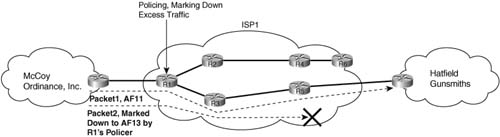
In the figure, two packets travel over a route marked with dotted lines. Each is marked with DSCP AF11 as they enter R1. R1’s policer decides that Packet1 conforms, but that Packet2 exceeds the policing rate. R1’s policer re-marks Packet2 as AF13. DiffServ suggests that AF13 should be in the same queuing class as AF11, but with a higher drop preference than AF11. If no congestion occurs, both packets get through the network. If some congestion occurs, however, Packet2 has a higher chance of being discarded, because it has a DSCP that implies a higher preference to be dropped than does Packet1.
Policing by marking down the packet provides a compromise option. The ISP can protect the network from being overrun by aggressively discarding marked-down packets at the onset of congestion. Customer satisfaction can be improved by letting the customers take advantage of the capacity when it is available.
The same concept, on a limited basis, can be applied in Frame Relay and ATM networks. Frame Relay headers include the discard eligibility (DE) bit, and ATM headers include the cell loss priority (CLP) bit. Each of these single bits can be used to imply that the frame or cell is a better frame or cell to discard when congestion occurs.
Finally, when choosing to re-mark a packet, you might actually want to mark multiple fields. For instance, you might want to mark down a packet from AF11 to AF13, inside the DSCP field of the IP header. You might also want to mark ATM CLP, or 802.1p CoS as well. When a policer is configured to mark multiple fields for packets that fall into a single policing category, the policer is said to be a multi-action policer.
Cisco IOS Software includes four different Shaping tools. Of those, CB Shaping and Frame Relay Traffic Shaping (FRTS) are the most popular. Interestingly, the four shaping tools all basically work the same way internally. In fact, the four shaping tools share much of the underlying shaping code in IOS. Although some features differ, and the configurations certainly differ, most of the core functions behave the same. So, rather than cover all four Traffic Shaping tools, the current QoS exam focuses on CB Shaping, which uses the Modular QoS command-line interface (MQC).
Note If you are interested in more information about FRTS, you can refer to Appendix B on the CD-ROM that comes with this book, which includes the old FRTS coverage from the first edition of this book.
CB Shaping has many features. First, the underlying processes, including the use of a single token bucket, work like the Shaping processes described earlier in this chapter. CB Shaping can be enabled on a large variety of interfaces. It can also adapt the rate based on BECN signals, and reflect BECNs on a VC after receiving an FECN. Additionally, CB Shaping can also perform shaping on a subset of the traffic on an interface. Finally, the configuration for CB Shaping is simple, because like all other QoS features starting with the words “class based,” CB shaping uses the Modular QoS command-line interface (MQC) for configuration.
In addition to its core features, CB Shaping can also take advantage of IOS queuing tools. Shapers queue traffic in order to slow the overall traffic rate. CB Shaping defaults to use a single FIFO queue when delaying packets, but it also supports several queuing methods for the shaping queues, including WFQ, CBWFQ, and LLQ. With these additional queuing tools, multiservice traffic can be better supported. For instance, LLQ can be applied to the shaping queues, providing a low-latency service for voice and video traffic.
As mentioned earlier, like all QoS tools whose names begin with “Class Based”, CB Shaping using MQC for configuration. Tables 6-7 and 6-8 list the configuration and show commands pertinent to CB shaping. The MQC match commands are omitted, but they can be found in Table 3-2 in Chapter 3.)


As usual, the best way to understand the generic commands is to see them used in an example. The first example configuration shows R3, with a 128-kbps access rate, and a 64-kbps Frame Relay VC connecting to R1. The criteria for the configuration is as follows:
![]() Shape all traffic at a 64Kbps rate.
Shape all traffic at a 64Kbps rate.
![]() Use the default setting for Tc.
Use the default setting for Tc.
![]() Enable the configuration on the subinterface.
Enable the configuration on the subinterface.
![]() Use WFQ on the physical interface.
Use WFQ on the physical interface.
![]() Use the default queuing method for the shaping queues.
Use the default queuing method for the shaping queues.
In each example, the client downloads one web page, which has two frames inside the page. The web page uses two separate TCP connections to download two separate large JPG files. The client also downloads a file using FTP get. In addition, a VoIP call is placed between extension 302 and 102. Example 6-1 shows the configuration and some sample show commands, and Figure 6-18 shows the network diagram.

Example 6-1 CB Shaping on R3, 64-kbps Shape Rate
class class-default
shape average 64000
interface serial0/0
bandwidth 64
load-interval 30
fair-queue
R3#show queue serial 0/0
Input queue: 0/75/1/0 (size/max/drops/flushes); Total output drops: 5965
Queueing strategy: weighted fair
Output queue: 0/1000/64/90 (size/max total/threshold/drops)
Available Bandwidth 1158 kilobits/sec
R3#show policy-map
Policy Map shape-all
Class class-default
Average Rate Traffic Shaping
CIR 64000 (bps) Max. Buffers Limit 1000 (Packets)
R3#show policy-map interface s0/0.1
Serial0/0.1
Service-policy output: shape-all
Class-map: class-default (match-any)
7718 packets, 837830 bytes
30 second offered rate 69000 bps, drop rate 5000 bps
Match: any
Target/Average Byte Sustain Excess Interval Increment
Rate Limit bits/int bits/int (ms) (bytes)
64000/64000 2000 8000 8000 125 1000
Active Depth Delayed Delayed Active
- 56 6393 692696 6335 684964 yes
The CB shaping configuration uses the default class (class-default), and a policy map (shape-all), which is enabled on serial 0/0.1 using the service-policy output shape-all command. The command class-map class-default matches all packets. The command policy-map shape-all only refers to the class-default class—essentially, classification is configured, but it matches all traffic. Inside class class-default, the shape average 64000 command shapes the traffic to 64 kbps.
Just like with other MQC-based tools, the show policy-map and show policy-map interface serial0/0.1 commands provide all the interesting information about this example. Note that show policy-map just lists the same information in the configuration, whereas show policy-map interface lists statistics, tells you whether shaping is currently active, and lists the computed values, such as Bc and Be in this case.
CB Shaping calculates a value for Bc and Be if the shape command does not include a value. From those values, CB Shaping calculates the Tc. At lower shaping rates (less than 320 kbps), CB Shaping assumes a Bc of 8000 bits, and calculates Tc based on the formula Tc = Bc/CIR, with some rounding as necessary. At 320 kbps, the calculated Tc would be 25 ms, or .025 seconds. Note that in this first example, Tc = 125 ms, because 8000/64,000 = 1/8 of a second.
For speeds higher than 320 kbps, CB Shaping instead uses a default Tc of .025 seconds, and calculates Bc based on the same formula, which with a little easy algebra translates to Bc = Tc * CIR. For instance, at 640 kbps, Bc = .025 * 640 kbps = 16,000 bits.
Note The QoS course currently suggests letting IOS pick Bc and Be values. If you are sending latency-sensitive multiservice traffic, you should set Bc to drive the calculation of Tc down to 10 ms. This recommendation has been made by Cisco in other documents.
A close examination of the output of the show policy-map interface s0/0.1 command in Example 6-1 provides a refresher of how Shaping works with its token bucket. First, Be defaults to be equal to Bc. Bc defaults to 8000 bits because the shaping rate (64 kbps) is less than 320 kbps. These two values are shown in the command output as Sustain bits/int and Excess bits/sec. Also note the heading Byte Limit—it represents the size of the token bucket. Bc + Be equals 16,000 bits, or 2000 bytes in this case. Finally, the last column in that same part of the command output lists Increment (bytes), which indicates how many bytes worth of tokens are replenished each Tc. The number of bits replenished into the token bucket each time period, and 8000 bits is of course equal to 1000 bytes. Essentially, the command output lists the details of how the Shaper’s token bucket logic will work.
In this example, packets are enqueued on the subinterface due to shaping, but few packets are enqueued on the physical interface software queues. With a 128-kbps clock rate, and a shaping rate for all traffic on the interface of 64 kbps, no congestion should occur on the physical interface.
By default, CB shaping uses simple FIFO Queuing for the shaping queue. A common misconception about CB shaping is that because the MQC commands are used, CBWFQ is automatically used — but that is not true! In this example, FIFO Queuing is used for the shaping queue.
You can explicitly set the Bc and Be values in addition to the shaping rate. As a result, you will have supplied two of the three variables in the Tc = Bc/CIR formula, and CB Shaping can simply calculate the Tc value implied by your configuration. The next example shows how to set Bc to affect Tc.
For the second configuration, imagine that the Frame Relay provider actually polices the VC from R3 to R1 at 96 kbps. You engineer the network to support a single G.729 VoIP call, which takes about 28 kbps. You decide that you want to be very careful about packet drops, latency, and jitter for this voice traffic, so you decide to shape all traffic except voice. To avoid drops inside the cloud, you shape the rest of the traffic to a rate of 64 kbps (so that the combined single VoIP call, and the Shaped rate of 64 kbps, do not exceed the policing rate in the Frame Relay network). The next example shows the configuration, and the criteria for the configuration is as follows:
![]() Shape non-VoIP traffic at 64 kbps.
Shape non-VoIP traffic at 64 kbps.
![]() Choose values so Tc is 50 ms.
Choose values so Tc is 50 ms.
![]() Enable the configuration on the subinterface.
Enable the configuration on the subinterface.
In this case, a single VoIP call and one web page connection with two frames inside the page are used, plus an FTP get. Example 6-2 shows the configuration and some sample show commands.
Example 6-2 CB Shaping on R3, 64-kbps for Non-Voice Traffic, Tc = 50 ms
!
match ip rtp 16384 16383
class voip-rtp
class class-default
shape average 64000 3200
interface serial0/0
bandwidth 64
load-interval 30
fair-queue
interface serial0/0.1
R3#show policy-map
Class voip-rtp
Class class-default
Traffic Shaping
Average Rate Traffic Shaping
CIR 64000 (bps) Max. Buffers Limit 1000 (Packets)
Bc 3200
R3#show policy-map interface serial 0/0.1
Serial0/0.1
Class-map: voip-rtp (match-all)
50379 packets, 3224256 bytes
Class-map: class-default (match-any)
5402 packets, 6634217 bytes
30 second offered rate 66000 bps, drop rate 0 bps
Match: any
Traffic Shaping
Target/Average Byte Sustain Excess Interval Increment
Rate Limit bits/int bits/int (ms) (bytes)
Adapt Queue Packets Bytes Packets Bytes Shaping
Active Depth Delayed Delayed Active
R3#show queue serial 0/0
Input queue: 0/75/0/0 (size/max/drops/flushes); Total output drops: 6083
Queueing strategy: weighted fair
Output queue: 0/1000/64/0 (size/max total/threshold/drops)
Available Bandwidth 1158 kilobits/sec
The configuration in the example is relatively simple, but detailed. It begins with some familiar MQC commands. The class-map match-all voip-rtp command creates a new class map, with parameters to match all VoIP payload traffic. The policy-map shape-non-voip command refers to class voip-rtp, with no parameters. With no parameters, no actions are taken for packets in the class, which includes no shaping action. class class-default refers to the class that matches all traffic, with the shape average 64000 3200 command shaping to 64 kbps, with a Bc of 3200 bits. (CB shaping then calculates Tc as 3200/64000, or 50 ms.) Note that because class voip-rtp occurs first in the policy map, all VOIP traffic matches that class, and is not shaped.
The show policy-map command just restates the information in the configuration. Note the absence of commands under class voip-rtp—remember, no commands were added under the command class voip-rtp—effectively creating a “do nothing” class. The class class-default command matches all other traffic, shaping to 64 kbps. In the show policy-map interface s0/0.1 command, you see that shaping is enabled only for class class-default, but not for class voip-rtp.
Note that Be, which was not configured, is defaulted to be equal to Bc as in the previous example.
While this example does show how CB Shaping can be configured to shape a subset of the traffic — which allows you to avoid shaping voice traffic—it also shows how to set Bc, and how it impacts the calculated Tc value. If you need to apply shaping in a network that includes VoIP traffic, the example in the next section shows a better choice for how to configure CB Shaping.
In the preceding example, the motivation to shape was based on the Frame Relay provider’s policing of the VC at 96 kbps. If the VoIP call was not active, the data still only gets 64 kbps worth of bandwidth! Although that’s great for the single voice call, it may not be a good choice for the data. The real requirement is for high-quality voice, with good treatment of the data as a secondary goal, knowing that the service provider is policing at 96 kbps.
A better solution is to use CB shaping’s capability to include CBWFQ or LLQ as the queuing tools for the shaping queues. In the first two examples, the shaping queue was a single FIFO queue, because no queuing was configured. In the next example, CB shaping will shape all traffic, including voice, at 96 kbps, but with LLQ used on the shaping queues to ensure good voice quality. Because it will shape voice traffic, this configuration forces Tc down to 10 ms, which is the recommended value for Tc when delay-sensitive voice and video traffic is shaped. The revised requirements are as follows:
![]() Ensure high-quality VoIP for one G.729 call, through low loss, low delay, and low jitter.
Ensure high-quality VoIP for one G.729 call, through low loss, low delay, and low jitter.
![]() Achieve VoIP loss goal by not exceeding the policing rate of the service provider.
Achieve VoIP loss goal by not exceeding the policing rate of the service provider.
![]() Achieve VoIP delay and jitter goal by using LLQ.
Achieve VoIP delay and jitter goal by using LLQ.
![]() Choose values so Tc is 10 ms.
Choose values so Tc is 10 ms.
![]() Shape all traffic, including voice, because LLQ will always take the voice traffic next anyway.
Shape all traffic, including voice, because LLQ will always take the voice traffic next anyway.
Example 6-3 shows the configuration.
Example 6-3 CB Shaping on R3, 96-kbps Shape Rate, with LLQ for Shaping Queues
!
!
! The following Policy map is used for queuing (LLQ)
class voip-rtp
priority 32
class class-default
fair-queue
!
!!!!!!!!!!!!!!!!!!!!!!!!!!!!!!!!!!!!!!!!!!!!!!!!!!!!!!!!!!!
! The following Policy map is used for Shaping;
! It refers to policy-map queue-voip
!
policy-map shape-all
class class-default
shape average 96000 960
service-policy queue-voip
interface serial0/0
bandwidth 64
load-interval 30
fair-queue
interface serial0/0.1
CIR 96000 (bps) Max. Buffers Limit 1000 (Packets)
Bc 960
Weighted Fair Queueing
Strict Priority
Bandwidth 32 (kbps) Burst 800 (Bytes)
Class class-default
Weighted Fair Queueing
Flow based Fair Queueing Max Threshold 64 (packets)
R3#show policy-map interface serial 0/0.1
Serial0/0.1
Class-map: class-default (match-any)
30 second offered rate 91000 bps, drop rate 0 bps
Match: any
Traffic Shaping
Target/Average Byte Sustain Excess Interval Increment
Rate Limit bits/int bits/int (ms) (bytes)
Adapt Queue Packets Bytes Packets Bytes Shaping
Active Depth Delayed Delayed Active
- 17 5172 910975 4002 831630 yes
Service-policy : queue-voip
4623 packets, 295872 bytes
Weighted Fair Queueing
Bandwidth 32 (kbps) Burst 800 (Bytes)
(pkts matched/bytes matched) 3528/225792
(total drops/bytes drops) 0/0
Weighted Fair Queueing
Flow Based Fair Queueing
Maximum Number of Hashed Queues 16
(total queued/total drops/no-buffer drops) 17/0/0
Example 6-3 contains a lot of interesting command output. It begins with the configuration, which is followed by several show commands. The configuration contains two policy maps; one configures shaping, and the other configures LLQ. Inside the shaping policy map (shape-all), the service-policy queue-voip command is used, which tells IOS to enable the queue-voip policy-map to the Shaping queues.
Because the interaction between the two policy maps can be confusing, Figure 6-19 shows the general idea behind what is happening in the configuration.
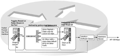
Scanning the figure from left to right, packets are first routed out the subinterface. Then the IOS checks to see whether shaping is active. Shaping becomes active when a single packet exceeds the traffic contract; shaping only becomes inactive when all the shaping queues are drained, and the ensuing packets are not exceeding the traffic contract. Therefore, the shaper must be involved at this step to decide whether to try to queue the packet into the shaping queue.
If the packet exceeds the contract, the shaper needs to queue the packet. In this case, instead of a single FIFO queue, you have a queuing system for the shaping queues as defined by policy-map queue-voip. This policy map defines two queues, with one being a 32-kbps low-latency queue into which all voice payload is placed. This queue was created with the class voip-rtp command inside policy-map queue-voip. Because queue-voip defines queuing, and no other details have been configured, all the rest of the packets go into a second queue, associated with the class-default class. (WFQ is applied to the packets inside the class-default queue, by default, but it can be disabled.)
The next step in the process really shows how integrated the queuing and shaping functions are in with this configuration. After packets have been enqueued in one of the shaping queues, CB shaping must decide when to take a packet from a queue. However, the shaper does not decide which packet to take — the queuing logic as defined in policy-map queue-voip determines which packet to dequeue next. Therefore, the shape average 96000 960 command tells CB shaping the rate and Bc values to use when deciding when it can next dequeue packets from the shaping queues. When CB shaping releases the next packet from the shaping queues, the packet is placed into the interface software queue, and it finally exits the serial interface.
The interaction between CB shaping, and the queuing tool used for the shaping queues (LLQ in this case) can be a bit confusing. In particular, the shaper must make the decision about whether to put a packet into the shaping queue, and then the shaper decides when the next packet can be taken from a shaping queue. Between those points, the queuing scheduler decides which packet to service next from the shaping queues.
Now taking a closer look at the configuration. The policy-map shape-all command creates the shaping configuration, with the shape average 96000 960 command enabling shaping and defining a Bc so that Tc = 960/96,000, or 10 ms. Although a Bc of 960 bits may seem smaller than a typical packet, you would typically also use a fragmentation tool on this interface when VoIP is in the network. Fragmentation would happen to cause the largest frame size to be shorter than 960 bits. In addition, the service-policy queue-voip command enables LLQ inside the class-default class inside policy map shape-all — thereby enabling LLQ for the shaping queues.
A closer look at policy-map queue-voip reveals two classes. The class voip-rtp command matches all VoIP payload, and is assigned 32 kbps with the priority 32 command, making it the low-latency queue. Remember, LLQ actually polices the traffic in the low-latency queue at this rate, so this queue can send only 32 kbps. Because all traffic is shaped at 96 kbps, 64 kbps remains, which is guaranteed for queuing; the class class-default command matches all other traffic, guaranteeing the remaining 64 kbps to the class.
Finally, the service-policy output shape-all subcommand on interface s 0/0.1 enables the policy on the subinterface, which enables CB shaping. Therefore, the CB shaping logic, and related LLQ logic, is applied to all packets exiting subinterface serial 0/0.1.
The show policy-map commands reflect the details in the configuration. The command lists policy-map shape-all as performing traffic shaping, and policy-map queue-voip as performing LLQ. The show policy-map interface s0/0.1 command lists the shaping parameters and statistics, just like it did in the earlier examples. However, halfway through the command output, a new section has appeared, with details about policy-map shape-all’s use of the LLQ policy-map queue-voip. The same information seen in CBWFQ and LLQ show policy-map interface commands in Chapter 4 appears in this area, including packet rates and byte rates.
This example allows the G.729 call to work well, because LLQ will always service the voip-rtp class when a packet is waiting. If no VoIP calls are up, however, the rest of the traffic can be sent at 96 kbps, the maximum sending rate for shaping. In other words, the rest of the traffic is guaranteed 64 kbps, with a maximum limit of the shaping rate. With LLQ, the VoIP always receives good treatment when the call is up, unless the VoIP traffic exceeds the LLQ policed rate of 32 kbps.
You should be aware of a couple of terms relating to this configuration on the test. When one policy map refers to another, the configuration are sometimes referred to as “hierarchical” policy maps. Other times, they are called “nested” policy maps. Or you can just think of it as how CBWFQ and LLQ can be configured for the shaping queues.
In all the examples of CB Shaping so far, the command that enabled shaping always began with the words shape average. However, there is another option instead of “average”, as seen in the generic form of the following command:
When you use the peak option, CB Shaping changes how it decides if a packet conforms to or exceeds the traffic contract. As a reminder, using the Shaping logic covered so far in this chapter, Bc bits are sent each Tc. If there’s been a period of low or no activity, and the Shaper has been configured with a Be value, then for a short time, more than Bc can be sent—specifically, Be more. With shape peak, the shaper allows Bc and Be bits to be sent in each interval, even if there has not been a period of little or no activity. In effect, shape peak means that the shaper actually shapes assuming you can send the configured burst during every time period.
Frankly, most people find how it works a little odd, so an example comparing shape average with shape peak, using the same settings, can help. First, consider shaping configured with the following command:
As covered earlier in this section, CB Shaping assumes a Bc of 8000, a Be of the same value, and then calculates Tc of .125 seconds. (Those numbers can be seen in Example 6-3.) The token bucket will be size Bc + Be, or 16,000 bits. After a period of inactivity, 16,000 bits can be sent. Under consistently high offered load, 8,000 bits can be sent each Tc, because the token bucket is filled at Bc bits (8000 bits) per interval.
Compare that to the following command to the shape average command:
Just as with shape average, CB Shaping assumes a Bc of 8000, a Be of the same value, and then calculates Tc of .125 seconds. And just as with shape average, the token bucket will be size Bc + Be, or 16,000 bits. However, instead of replenishing the token bucket with Bc bits each Tc, shape peak tells CB Shaping to replenish Bc + Be tokens per Tc. Translated, that means that the shaper gets the right to send the committed burst, and the excess burst, every time period.
Interestingly, the shape peak 64000 command actually shapes packets at a rate higher than 64 kbps. To calculate the actual rate, you would use the following formula:
![]()
For instance, in this example, the actual shaping rate would be 128 kbps:
![]()
Example 6-4 lists an example configuration using shape peak, along with a few comments confirming the math behind the use of this command.

To interpret the example, first remember that Bc defaults to 8000 bits at speeds lower than 320 kbps, and that Be = Bc by default. The show policy-map interface s0/0 command lists the target rate as 128,000 bits/second, as confirmed with the math that precedes the example. Also, the column labeled Increment (bytes) refers to the number of bytes worth of tokens added back to the token bucket in each interval. To support the peak rate, instead of just adding Bc worth of tokens (1000 bytes), Bc + Be (2000 bytes) worth of tokens are added.
This chapter covered the concepts behind adaptive shaping a little earlier. To configure adaptive shaping with CB Shaping, you need to use the shape command twice inside a single policy-map. Example 6-5 shows an example:
Example 6-5 Adaptive CB Shaping Configuration
policy-map shape-all
class class-default
shape adaptive 32000!
bandwidth 64
load-interval 30
fair-queue
interface serial0/0.1
As you can see in the example, the shape average command is configured, along with the shape adaptive command, inside the same policy map class (class-default). The shape average command enables shaping; with that command alone, CB Shaping shapes at 96 kbps all the time. With shape adaptive 32000 configured in the same class, CB Shaping will reduce the shaping rate in reaction to received BECNs, all the way down to 32 kbps. The rate is reduced by 25 percent of the previous actual shaping rate for each BECN received. But the shaping rate will never fall below 32 kbps—so you can think of that rate as the minimum rate, and the 96-kbps rate as the maximum rate.
As a reminder, after 16 consecutive intervals with no received BECNs, this router would start increasing the Shaping rate by 1/16 of the original 96-kbps shaping rate each Tc. To do so, CB Shaping actually starts replenishing the token bucket with a little more each Tc, specifically by (Bc + Be)/16 each Tc. As a result, the rate will likely increase a little more slowly than it decreased in the presence of BECNs.
The shape command also allows you to configure the shaping rate based on a percentage of link bandwidth, if you prefer. That’s true whether or not you are configuring CB shaping with the shape average or shape peak commands. For instance, if you had a Frame Relay interface whose access rate (the physical clock rate) was 128 kbps, but you wanted to configure shaping for 64 kbps, you could use the shape average percent 50 command.
Be aware that the calculation of the actual shaping rate, when enabled on a physical interface, is based on the interface’s configured bandwidth. For instance, in this same example, the default setting of the interface’s bandwidth command is 1544, meaning T/1 speed. The shaping rate would then be calculated as 50 percent of that, or 772 kbps.
Note also that with the percent option, Bc and Be are configured with units of milliseconds. Interestingly, configuring Bc with the percent option actually sets Tc, with CB Shaping calculating Bc based on the Bc = Tc * CIR formula. Example 6-6 shows an example configuration, along with the calculated Bc and Be values.

In the configuration, the shape average percent 50 125 ms command enables shaping for a rate of 50 percent of the interface’s bandwidth. In this case, on S0/1, the bandwidth has been set to 128 kbps, so when the service-policy output percent-test command is used, CB Shaping calculates the rate as 50 percent of 128 kbps. Please note that the command requires the ms keyword after the number of ms configured for the Bc value (as shown), and for the Be value (not shown in this example.)
The output of the show policy-map interface command lists several interesting bits of information as well. For instance, note that the calculated rate of 64000 bits/second is shown. Also, the configured Bc time period of 125 ms shows up as the time interval. CB Shaping then calculated Bc = 64,000 * .125, or 8000 bits.
The QoS exam does not cover the other three IOS shaping tools, other than a possible need to simply know about the existence of GTS, DTS, and FRTS. Interestingly, the QoS exam does cover Frame Relay Fragmentation, which happens to require FRTS configuration, so you may want to glance over the FRTS coverage in Appendix B which is found on the CD-ROM.
It is good to review the features of CB Shaping now that you have read about the concepts and the configuration. At the same time, because many installations still use FRTS, it seems appropriate to compare the two QoS tools here, in spite of the fact that the exam objectives certainly don’t mention FRTS.
Table 6-9 summarizes the key points for comparison between the CB Shaping and FRTS, with a few words of explanation following.
Table 6-9 Comparison of CB Shaping and FRTS Features

* The Cisco QoS course claims WFQ is supported on the physical interface. In addition, FRF is not technically a queuing tool, although its feature of using two queues does achieve the same effect.
A few words explaining the content of the table can help. First, FRTS only supports Frame Relay—otherwise it’d be a really poor choice of name—but CB Shaping supports any type of data link protocol. If you configure Frame Relay to use multipoint subinterfaces, FRTS does allow you to shape for each VC, whereas CB Shaping does not.
Another point that used to be very important, but isn’t today, relates to CB Shaping’s non-support of Frame Relay fragmentation. Fragmentation, covered in Chapter 8 of this book, is very important for supporting latency-sensitive traffic. However, there is a fragmentation option available, called Multi-link PPP over Frame Relay Fragmentation, which allows CB Shaping to be used on Frame Relay interfaces concurrently with fragmentation.
CB policing performs policing using three separate actions for packets that conform, exceed, or violate the traffic contract. (The exact meanings of each of these three categories were covered in the “How Policing Works” section earlier in this chapter.) Generally speaking, CB policing considers packets that happen to arrive when enough Bc tokens are available as “conforming” packets. Packets that arrive when Bc is consumed, but Be is not, are considered “exceeding”; and packets that arrive after Bc and Be have been consumed are considered “violating” packets.
For each category (conform, exceed, violate), CB policing can use a variety of actions. Table 6-11, a little later in the chapter, lists the action keywords used in the police command. In general, the choices are to drop the packet, transmit the packet, or to first re-mark some QoS field, and then transmit the packet. CB policing uses MQC commands for configuration. Because it is class based, CB policing can police subsets of the traffic on the interface or subinterface on which it is enabled. CB policing uses the same familiar MQC classification commands that all the other MQC-based tools use; again, you only need to learn one more MQC command to know how to configure another MQC QoS feature.
The police command configures CB policing inside a policy map. On the police command, you define the policing rate in bps, the Bc in bytes, and the Be in bytes. Note that CB Shaping’s settings for Bc and Be were in bits, not bytes!
Two examples of configuration for CB policing (Examples 6-7 and 6-8) follow Tables 6-10 through 6-12. Table 6-10 lists the CB policing configuration commands. Table 6-11 lists the actions that you can configure on the police command. (The MQC match commands, which can be used with any of the MQC-based features, are not listed, but can be seen in Table 3-2 in Chapter 3.) Table 6-12 lists the CB policing show commands.

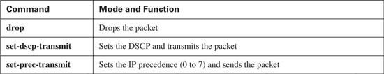


The actions to take on each packet, whether it conforms, exceeds, or violates the contract, boil down to either dropping the packet, transmitting the packet, or re-marking and transmitting the packet. The drop and transmit options are pretty obvious. However, CB policing includes keywords such as set-prec-transmit and set-dscp-transmit, which allow the policer to transmit the packet, but first mark the IP Precedence or DSCP field with a lower value. You may recall from the “How Policing Works” section that marking down a packet can be useful because the marked-down packet can have a higher likelihood for discard later, but if no congestion occurs, the packet can be delivered. You can also configure CB Policing to use multiple actions, for instance, mark DSCP and LAN CoS for packets that exceed the contract.
You can use CB policing to police all traffic, or a subset of the traffic, entering or exiting an interface. In the first example, router ISP-edge polices all ingress traffic from an enterprise network. The criteria for the first CB policing example is as follows:
![]() Create a single-rate, three-color policing configuration.
Create a single-rate, three-color policing configuration.
![]() All traffic policed at 96 kbps at ingress to the ISP-edge router.
All traffic policed at 96 kbps at ingress to the ISP-edge router.
![]() Bc of 1 second’s worth of traffic is allowed.
Bc of 1 second’s worth of traffic is allowed.
![]() Be of 0.5 second’s worth of traffic is allowed.
Be of 0.5 second’s worth of traffic is allowed.
![]() Traffic that violates the contract is discarded.
Traffic that violates the contract is discarded.
![]() Traffic that exceeds the contract is marked down to DSCP Be.
Traffic that exceeds the contract is marked down to DSCP Be.
![]() Traffic that conforms to the contract is forwarded with no re-marking.
Traffic that conforms to the contract is forwarded with no re-marking.
Figure 6-20 shows the network in which the configuration is applied, and Example 6-7 shows the configuration.

Example 6-7 Single-rate Three-color CB Policing at 96 kbps at ISP-edge Router
Building configuration...
!
!Lines omitted for brevity
!
ip cef
!
class class-default
! note: the police command wraps around to a second line.
police cir 96000 bc 12000 be 6000 conform-action transmit exceed-action
set-dscp- transmit 0 violate-action drop
interface Serial1/0
description connected to FRS port S1. Single PVC to R3.
no ip address
encapsulation frame-relay
load-interval 30
clockrate 1300000
!
interface Serial1/0.1 point-to-point
description point-point subint global DLCI 101, connected via PVC to Ent-edge
ip address 192.168.2.251 255.255.255.0
frame-relay interface-dlci 103
!
! Lines omitted for brevity
!
ISP-edge#show policy-map
Policy Map police-all
Class class-default
! wraps around to a second line.
transmit exceed-action set-dscp-transmit 0 violate-action drop
ISP-edge#show policy-map interface s 1/0
Serial1/0
Service-policy input: police-all
Class-map: class-default (match-any)
8375 packets, 1446373 bytes
30 second offered rate 113000 bps, drop rate 15000 bps
Match: any
cir 96000 bps, conform-burst 12000, excess-burst 6000
conformed 8077 packets, 1224913 bytes; action: transmit
exceeded 29 packets, 17948 bytes; action: set-dscp-transmit 0
violated 269 packets, 203512 bytes; action: drop
conformed 95000 bps, exceed 0 bps violate 20000 bps
The example takes advantage of the fact that in any policy map, all traffic that does not match a class gets placed into the class-default class. Because one design goal was to police all traffic, no explicit class maps were needed—all traffic matches the class-default class inside every policy map by default. Therefore, inside new policy map police-all, the police cir 96000 bc 12000 be 18000 conform-action transmit exceed-action set-dscp-transmit 0 violate-action drop command enables policing for the class-default class.
The parameters of the police command set the policing rate to 96,000 bps, with 12,000 bytes of burst capability. The shaping tools configure Bc and Be as a number of bits; IOS policers configure these values as a number of bytes. The requirements for this example stated 1 second’s worth of Bc, and 12,000 bytes can be sent in 1 second with a CIR of 96,000 bps. The excess-burst configuration parameter is 6000 bytes, or half of Bc. The stated goals asked for a Be of 0.5 seconds of traffic, and it does indeed take 0.5 seconds to send 6000 bytes at 96 kbps.
Keep in mind that all IOS shapers use bits as the unit when setting Bc and Be; both policers use bytes as the unit.
The police command defines a single rate, but the fact that it is a three-color policing configuration, and not a two-color configuration, is not obvious at first glance. To configure a three-color policer, you need to either configure a Be value larger than 0, or configure a violate action, or both. In this case, both are configured, telling IOS to use two token buckets, thereby enabling three categories for the packets.
In Example 6-7, the police command transmits packets that conform, marks down packets that exceed to a DSCP value of zero, and drops packets that violate the values. The show policy- map command repeats the same details as shown in the configuration command, as highlighted in the example. The show policy-map interface s1/0 command lists statistics about the number of packets that conformed, exceeded, and violated the contract.
One of the advantages of CB policing is the ability to perform policing per class. The next example, Example 6-8, shows CB policing with web traffic classified and policed differently than the rest of the traffic. The criteria for the next CB policing example is as follows:
![]() Police web traffic at 80 kbps at ingress to the ISP-edge router. Transmit conforming and exceeding traffic, but discard violating traffic.
Police web traffic at 80 kbps at ingress to the ISP-edge router. Transmit conforming and exceeding traffic, but discard violating traffic.
![]() Police all other traffic at 16 kbps at ingress to the ISP-edge router. Mark down exceeding and violating traffic to DSCP 0.
Police all other traffic at 16 kbps at ingress to the ISP-edge router. Mark down exceeding and violating traffic to DSCP 0.
![]() Bc of 1 second’s worth of traffic is allowed.
Bc of 1 second’s worth of traffic is allowed.
![]() Be of 0.5 second’s worth of traffic is allowed.
Be of 0.5 second’s worth of traffic is allowed.
Example 6-8 shows the configuration.
Example 6-8 CB Policing 80 kbps for Web Traffic, 16 kbps for the Rest with Markdown to Be, at ISP-edge Router
Building configuration...
!
!Lines omitted for brevity
!
ip cef
!
match protocol http
class match-web
police cir 80000 bc 10000 be 5000 conform-action transmit exceed-action transmit
violate-action drop
class class-default
police cir 16000 bc 2000 be 1000 conform-action transmit exceed-action
transmit violate-action set-dscp-transmit 0
interface Serial1/0
description connected to FRS port S1. Single PVC to R3.
no ip address
ip nbar protocol-discovery
encapsulation frame-relay
load-interval 30
clockrate 1300000
!
interface Serial1/0.1 point-to-point
description point-point subint global DLCI 101, connected via PVC to DLCI 103 (R3)
ip address 192.168.2.251 255.255.255.0
frame-relay interface-dlci 103
!
!
!Lines omitted for brevity
!
ISP-edge#show policy-map
Policy Map police-web
! note: the police command wraps around to a second line.
police cir 80000 conform-burst 10000 excess-burst 5000 conform-action
transmit exceed-action transmit violate-action drop
Class class-default
! note: the police command wraps around to a second line.
transmit exceed-action transmit violate-action set-dscp-transmit 0
ISP-edge#show policy-map interface s 1/0
Serial1/0
Service-policy input: police-web
30 second offered rate 90000 bps, drop rate 14000 bps
Match: protocol http
cir 80000 bps, conform-burst 10000, excess-burst 5000
conformed 625 packets, 748645 bytes; action: transmit
exceeded 13 packets, 14268 bytes; action: transmit
violated 98 packets, 137592 bytes; action: drop
conformed 75000 bps, exceed 0 bps violate 17000 bps
30 second offered rate 26000 bps, drop rate 0 bps
Match: any
cir 16000 bps, conform-burst 2000, excess-burst 1000
conformed 2330 packets, 149928 bytes; action: transmit
exceeded 46 packets, 2944 bytes; action: transmit
violated 1376 packets, 88808 bytes; action: set-dscp-transmit 0
conformed 16000 bps, exceed 0 bps violate 9000 bps
If you are becoming comfortable with MQC configurations now, this configuration should be relatively easy to decipher. The class-map match-all match-web command creates a new class, which matches all web traffic using NBAR. The policy-map police-web command creates a new policy map, which uses class match-web to classify web traffic, and class class-default to classify all other traffic.
Inside each class of the policy-map, a police command is used, setting the parameters as outlined in the stated goals. For instance, the police cir 80000 bc 10000 be 5000 conform- action transmit exceed-action transmit violate-action drop command sets the rate at 80 kbps, with a 1-second Bc value of 10,000 bytes, and a configured Be of 5,000 bytes.
The show policy-map interface s1/0 command lists statistics as always, in this case showing the two classes in the policy map police-web. As you would expect, separate policing statistics are shown per class, because CB policing is enabled per class.
The first two examples in this section on CB Policing configuration showed single rate policing with two token buckets. By using two token buckets, CB Policing could create three categories for the packets—conforming, exceeding, and violating. Using terminology from RFC 2496, CB Policing was configured as a single-rate three-color policer in each case, with the word “color” implying the three categories (conform, exceed, violate).
Note To create a single rate two-color CB Policing configuration, you simply do not include the violate-action keyword and the Be value in the police command.
This section shows an example of configuring a dual-rate three-color policer. As you might recall from the earlier section titled “CB Policing: Dual Rates, Three-Color (2 Buckets)”, a dual-rate policer uses two rates, one called CIR, and one called PIR. The goal of a dual-rate policer is to let the engineer define the two rates, with packets below the CIR considered to conform, packets above CIR but below PIR considered to exceed, and all other packets considered to violate the contract.
To allow configuration of two different rates, the police command is still used. However, the syntax differs slightly from the earlier use of the command. The generic syntax is as follows:
[conform-action action [exceed-action action [violate-action action]]]
Note that with the syntax of this command, you are required to configure a CIR and a PIR setting. (The curly brackets mean that the parameter is required.) The command includes a place to set the Bc value and the Be values as well, plus the same set of options for conform, exceed, and violate actions.
For example, if you wanted to perform dual-rate policing, with a CIR of 96 kbps and a PIR of 128 kbps, you would simply use a command like police cir 96000 pir 128000.
There are a few more miscellaneous points you should be aware of with CB Policing. This short section outlines the remaining points.
If a packet violates the contract, instead of discarding it, you might mark down DSCP to 0. That way, if the rest of the network is not congested, the packet makes it through, but if the network is congested, another router will be more likely to discard the packet.
On occasion, an engineer might want to mark more than one field in a packet header. For instance, Frame Relay switches might choose to discard frames with DE marked in the Frame Relay header, rather than those with DE unmarked, if congestion does occur. An engineer might want to mark both DSCP and FR DE when a packet violates the contract.
Cisco supports marking multiple fields for a single category with policing. To do so, first the police command is used to set the rate(s), but the actions are not configured in the police command. Instead, by omitting the actions, the police command places the user into another submode, in which the actions can be added on individual lines. To configure multiple actions, multiple conform-action, exceed-action, or violate-action subcommands are used. Example 6-9 shows an sample, with marking of DSCP 0 and FR DE for packets that violate the traffic contract:
Example 6-9 Multi-action Policing
Enter configuration commands, one per line. End with CNTL/Z.
R3(config)#policy-map testpol1
R3(config-pmap)#class class-default
R3(config-pmap-c)#police 128000 256000
R3(config-pmap-c-police)#conform-action transmit
R3(config-pmap-c-police)#exceed-action transmit
R3(config-pmap-c-police)#violate-action set-dscp-transmit 0
R3(config-pmap-c-police)#violate-action set-frde-transmit
Note that the preceding is not a single police command, but instead, it uses a sub-command mode after the police command. In particular, note that there are two instances of the violate-action subcommand, with different actions listed.
Like for the shape command, IOS supports a version of the police command that allows you to configure the policing rate as a percentage of link bandwidth. You can also configure the Bc and Be values as a number of milliseconds, from which IOS calculates the actual Bc and Be values based on how many bits can be sent in that many milliseconds. Example 6-10 shows an example of a dual-rate policing configuration using the percentage option.
Example 6-10 Configuring Percentage-Based Policing
! Portions omitted for Brevity
policy-map test-pol6
class class-default
!
interface serial0/0
bandwidth 256
R3#show policy-map interface s0/0
Serial0/0
Service-policy output: test-pol6
Class-map: class-default (match-any)
4 packets, 156 bytes
5 minute offered rate 0 bps, drop rate 0 bps
Match: any
cir 25 % bc 500 ms
cir 64000 bps, bc 4000 bytes
pir 50 % be 500 ms
pir 128000 bps, be 8000 bytes
transmit
exceeded 0 packets, 0 bytes; actions:
drop
violated 0 packets, 0 bytes; actions:
drop
conformed 0 bps, exceed 0 bps, violate 0 bps
R3#
The syntax of the police command includes the percent keyword, telling IOS to interpret the CIR and PIR values as link percentages. Once enabled on interface serial0/0, which has a bandwidth 256 command, IOS can interpret the percentages into actual bit rates. For instance, the output of the show policy-map interface s0/0 command lists CIR as 25 percent on one line, and then as 64000 bps on the next. The math is simply the percentage times the interface bandwidth, or 25 percent of 256 kbps. The PIR is calculated the same way, in this case as 50 percent of the PIR, or 50 percent of 256 kbps.
Note that the Bc and Be values are configured as a number, followed by the keyword ms (meaning milliseconds). To calculate the actual Bc and Be, the math is again simple. IOS figures out how many bits would be sent in that many milliseconds at the stated rate. For instance, Bc was set to 500 ms; at a CIR of 64 kbps, you can send 32,000 bits in 500 ms (.5 seconds times 64,000 bits/second). So Bc is calculated as 32,000 bits, but for policing, Bc and Be units are bytes—so the show policy-map interface command lists a Bc of 4,000 bytes. Similarly, the Be is calculated as PIR * number_of_milliseconds, or 128,000 bits/second multiplied by .5 seconds, or 64,000 bits. Converted to bytes, that’s 8000 bytes, which is indeed reflected in the show policy-map interface command output in the example.
If you do not configure a Bc value, then CB Policing configures a default value based on the following formula:
![]()
Although the math is easy, this formula may seem to be a little random at first. What logic behind it is essentially to figure out how many bytes could be sent at the CIR speed in 1/4 of a second. And remember, the CIR is in bits/second, and the Bc setting is in bytes. So, a different look at the formula may make more sense:
![]()
Also note that CB Policing will not allow the calculated default to be less than 1500—if the math works out to a number less than 1500, CB Policing uses 1500 instead.
For Be, the default depends on whether you configure a single bucket (two color) policer, or a two bucket (three color) policer. To configure to use a single bucket/two colors, just leave off the Be and violate-action options. In this case, Be defaults to 0. However, if you configure a violate action, or set Be to something besides 0, IOS thinks you want to use a two bucket/three color policing function. In that case, IOS defaults Be = Bc.
When dual-rate policing is used, and Bc and Be are not configured, IOS calculates the value for Bc using the same formula as shown previously. For Be, IOS using a slightly-different formula, with the same intent, but based on PIR:
![]()
Table 6-13 summarizes the small details about the defaults for Bc and Be. The table lists all three cases, plus a reminder of how to know which style of configuration is being used.

Like the shape command, the police command now includes an option for configuring the rate using a percentage of link bandwidth. The concept works the same way as it does the shape command. For instance, if an interface had a bandwidth setting of 128 kbps, to police at 64 kbps, the police cir percent 50 command could be used. The generic form of the police command, using the percent option, is as follows:
[be peak-burst-in-msec] [conform-action action [exceed-action action
[violate-action action]]]
When using the police command with the percent option, you only have to configure the CIR percentage. To configure a single-rate policer, simply don’t include the pir option; to configure a dual-rate policer, include the pir option. Regardless of whether the command defines single-rate or dual-rate policing, if Bc and Be are not configured, IOS calculates the value to use for each using the same rules as described in the previous section of this chapter.
CB Policing inside Cisco IOS has many features, most of which are covered in this chapter. The syntax of the commands, the ways the police command can be used, and the meaning of the output of the related show commands are all important. Also, the core features of how Cisco implements CB Policing in Cisco IOS are also important, and are summarized in the list that follows.
![]() Supports Single-rate, two-color policing, which uses a single token bucket, and two action categories (conform and exceed)
Supports Single-rate, two-color policing, which uses a single token bucket, and two action categories (conform and exceed)
![]() Single-rate, three-color policing, which uses two token buckets, and three action categories (conform, exceed, and violate)
Single-rate, three-color policing, which uses two token buckets, and three action categories (conform, exceed, and violate)
![]() Dual-rate, three-color policing, using two buckets, supporting both CIR and PIR rates
Dual-rate, three-color policing, using two buckets, supporting both CIR and PIR rates
![]() “Two Color” and “Three color” terminology refers to the actions categories that can be determined by the policer – namely conform, exceed, and violate
“Two Color” and “Three color” terminology refers to the actions categories that can be determined by the policer – namely conform, exceed, and violate
![]() Supports policing of a subset of traffic by using MQC classes, with the police command enabled in the traffic classes that include the packets that need to be policed
Supports policing of a subset of traffic by using MQC classes, with the police command enabled in the traffic classes that include the packets that need to be policed
![]() Support for multiactions policing by repeating the conform-action, exceed-action, and/or violate-action keywords.
Support for multiactions policing by repeating the conform-action, exceed-action, and/or violate-action keywords.
![]() For single-rate policing, if Bc and Be are not configured, IOS calculates the values as Be = 0 and Bc as the larger of either 1500 or CIR/32.
For single-rate policing, if Bc and Be are not configured, IOS calculates the values as Be = 0 and Bc as the larger of either 1500 or CIR/32.
![]() For dual-rate policing, if Bc and Be are not configured, IOS calculates the values as follows: Bc as the larger of either 1500 or CIR/32, and Be as the larger of either 1500 or PIR/32.
For dual-rate policing, if Bc and Be are not configured, IOS calculates the values as follows: Bc as the larger of either 1500 or CIR/32, and Be as the larger of either 1500 or PIR/32.
![]() The police command allows configuration of the rates as percentages of link bandwidth, with Bc and Be being set as a number of milliseconds.
The police command allows configuration of the rates as percentages of link bandwidth, with Bc and Be being set as a number of milliseconds.
The “Foundation Summary” is a collection of tables and figures that provide a convenient review of many key concepts in this chapter. For those of you already comfortable with the topics in this chapter, this summary could help you recall a few details. For those of you who just read this chapter, this review should help solidify some key facts. For any of you doing your final prep before the exam, these tables and figures are a convenient way to review the day before the exam.
ISPs make the business choice of whether to police, and how aggressively to police. The options reduce to the following three basic options:
![]() Do not police. To support the traffic, build the network to support the traffic as if all customers will send and receive data at the clock rate of the access link. From a sales perspective, close deals by claiming that no policing will be done, but encourage customers who exceed their contracts to pay for more bandwidth.
Do not police. To support the traffic, build the network to support the traffic as if all customers will send and receive data at the clock rate of the access link. From a sales perspective, close deals by claiming that no policing will be done, but encourage customers who exceed their contracts to pay for more bandwidth.
![]() Police at the contracted rate. To support these traffic levels, the network only needs to be built to support the collective contracted rates, although the core would be overbuilt to support new customers. From a sales perspective, encourage customers that are beginning to exceed their contracts to upgrade, and give incentives.
Police at the contracted rate. To support these traffic levels, the network only needs to be built to support the collective contracted rates, although the core would be overbuilt to support new customers. From a sales perspective, encourage customers that are beginning to exceed their contracts to upgrade, and give incentives.
![]() Police somewhere in between the contracted rate and the access-link clock rate. For instance, ISP1 might police PB Tents at 5 Mbps, when the contract reads 2 Mbps. The network can be built to support the collective policed rates. The sales team can encourage customers to buy a larger contracted rate when they consistently exceed the contracted rate, but keep customer satisfaction higher by pointing out their generosity by only policing at rates much higher than the contracted rates.
Police somewhere in between the contracted rate and the access-link clock rate. For instance, ISP1 might police PB Tents at 5 Mbps, when the contract reads 2 Mbps. The network can be built to support the collective policed rates. The sales team can encourage customers to buy a larger contracted rate when they consistently exceed the contracted rate, but keep customer satisfaction higher by pointing out their generosity by only policing at rates much higher than the contracted rates.
Figure 6-21 points out two cases of egress blocking, using a Frame Relay network as an example.

Table 6-14 summarizes some of the key points about when and where you should consider using policing and shaping.

Traffic shaping implements this basic logic by defining a measurement interval, and a number of bits that can be sent in that interval, so that the overall shaped rate is not exceeded. Table 6-15 lists some related definitions.

Traffic Shaping uses a token bucket to control the mechanics of deciding which packets conform to the shaping rate, and which exceed the rate. Two main actions revolve around the token bucket and the tokens:
![]() The re-filling of the bucket with new tokens
The re-filling of the bucket with new tokens
![]() The consumption of tokens by the Shaper to gain the right to forward packets.
The consumption of tokens by the Shaper to gain the right to forward packets.
For filling the token bucket, the bucket is filled to the brim, but no more, at the beginning of each Tc (assuming that Be = 0 for the time being). Another way you can think of it as if the Shaper dumps Bc worth of tokens into the Bucket at the beginning of every interval—but if there’s not enough room in the bucket, because not all the tokens were used during the previous time interval, some tokens spill out—and those spilled tokens can’t be used. The net result, either way you look at it, is that the interval starts with a full token bucket of size Bc. Figure 6-22 shows the basic idea:

With Be configured, the size of the single token bucket used by shaping is Bc + Be, but the tokens are still only refilled with Bc every time interval. This effectively lets the shaper save extra tokens after a period of inactivity in order to burst longer. Figure 6-23 lists the overall process used by shaping, with both a Bc and Be value configured.

The formulas IOS uses to calculate Tc when you configure both the shaping rate and the Bc are as follows:
![]()
Or
![]()
CB Shaping calculates a value for Bc and Be if the shape command does not include a value. From that, it calculates the Tc. At lower shaping rate (less than 320Kbs), CB Shaping assumes a Bc of 8000 bits, and calculates Tc based on the formula Tc = Bc/CIR, with some rounding as necessary. Note that at 320 kbps, the calculated Tc would be 25 ms, or .025 seconds.
For speeds higher than 320 kbps, CB Shaping instead uses a default Tc of .025 seconds (250 ms), and calculates Bc based on the same formula, which with a little easy algebra translates to Bc = Tc * CIR. For instance, at 640 kbps, Bc = .025 * 640 kbps = 16,000 bits.
CB Shaping defaults Be to be equal to Bc.
CB Shaping can adapt its shaping rate based on the receipt of BECNs or Foresight messages. When the shaper receives a BECN or Foresight message, it slows down by 25 percent of the maximum rate, repeating the process for each received BECN or Foresight message, until the minimum rate is reached. The rate grows again after 16 consecutive intervals occur without a BECN or Foresight congestion message. The shaping rate grows by 1/16 of the maximum rate during each Tc, until the maximum rate is reached again. This process results in an increase in the shaping rate based on the following formula: (Bc + Be)/16.
When a shaper uses a queuing tool, instead of having a single shaping queue, multiple shaping queues exist. If FRTS were configured to use PQ, for example, up to four queues could be created for shaping. Figure 6-24 shows the basic idea, with shaping enabled on the physical interface, FIFO Queuing on the physical interface, and PQ configured for the shaping queue.

Many QoS designs call for shaping per VC. For the same router, with two 64-kbps CIR VCs (each configured on a separate point-to-point subinterface) shaping queues are created for each subinterface, with the familiar output queues as well. Figure 6-25 depicts the overall idea.

The CB Shaping shape command has an option for peak-rate shaping. For instance, the shape peak 64000 command actually shapes packets at a rate higher than 64 kbps. To calculate the actual rate, you would use the following formula:
![]()
For instance, the actual shaping rate would be 128 kbps, assuming the default value 8000 for both Bc and Be:
![]()
Table 6-16 summarizes the key points for comparison between the CB Shaping and FRTS, with a few words of explanation following.
Table 6-16 Comparison of CB Shaping and FRTS Features
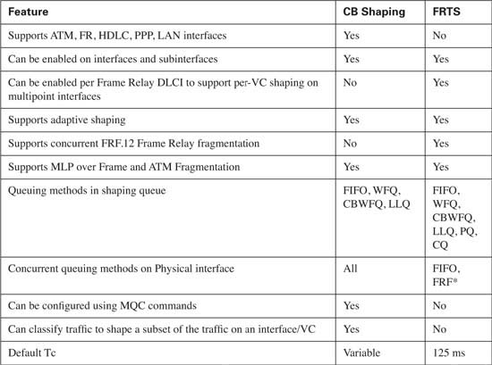
* The Cisco QoS course claims WFQ is supported on the physical interface. In addition, FRF is not technically a queuing tool, although its feature of using two queues does achieve the same effect.
CB Policing includes a lot of small details about how it chooses which packets conform to, exceed, or violate a traffic contract. To help with exam prep, Table 6-17 lists the key points about how CB Policing uses token buckets.
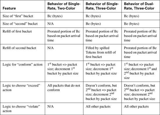
Figure 6-26 shows how a single-rate, three-color policer replenishes the tokens in the dual token buckets.

Figure 6-27 depicts the mechanics of how a dual-rate, three-color policer works in regards to refilling tokens into the dual token buckets:
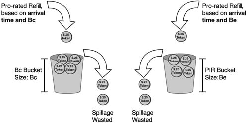
Table 6-18 summarizes the small details about the defaults for Bc and Be. The table lists all three cases, plus a reminder of how to know which style of configuration is being used.

Table 6-19 lists the various actions associated with CB policing.
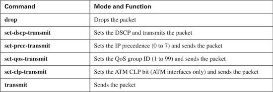
The list that follows summarizes the core features of how Cisco implements CB Policing.
![]() Supports Single-rate, two-color policing, which uses a single token bucket, and two action categories (conform and exceed)
Supports Single-rate, two-color policing, which uses a single token bucket, and two action categories (conform and exceed)
![]() Single-rate, three-color policing, which uses two token buckets, and three action categories (conform, exceed, and violate)
Single-rate, three-color policing, which uses two token buckets, and three action categories (conform, exceed, and violate)
![]() Dual-rate, three-color policing, using two buckets, supporting both CIR and PIR rates
Dual-rate, three-color policing, using two buckets, supporting both CIR and PIR rates
![]() “Two Color” and “Three color” terminology refers to the actions categories that can be determined by the policer – namely conform, exceed, and violate
“Two Color” and “Three color” terminology refers to the actions categories that can be determined by the policer – namely conform, exceed, and violate
![]() Supports policing of a subset of traffic by using MQC classes, with the police command enabled in the traffic classes that include the packets that need to be policed
Supports policing of a subset of traffic by using MQC classes, with the police command enabled in the traffic classes that include the packets that need to be policed
![]() Support for multiactions policing by repeating the conform-action, exceed-action, and/or violate-action keywords.
Support for multiactions policing by repeating the conform-action, exceed-action, and/or violate-action keywords.
![]() For single-rate policing, if Bc and Be are not configured, IOS calculates the values as Be = 0 and Bc as the larger of either 1500 or CIR/32.
For single-rate policing, if Bc and Be are not configured, IOS calculates the values as Be = 0 and Bc as the larger of either 1500 or CIR/32.
![]() For dual-rate policing, if Bc and Be are not configured, IOS calculates the values as follows: Bc as the larger of either 1500 or CIR/32, and Be as the larger of either 1500 or PIR/32.
For dual-rate policing, if Bc and Be are not configured, IOS calculates the values as follows: Bc as the larger of either 1500 or CIR/32, and Be as the larger of either 1500 or PIR/32.
![]() The police command allows configuration of the rates as percentages of link bandwidth, with Bc and Be being set as a number of milliseconds.
The police command allows configuration of the rates as percentages of link bandwidth, with Bc and Be being set as a number of milliseconds.
As mentioned in the Introduction, you have two choices for review questions. The questions that follow next give you a more difficult challenge than the exam itself by using an open-ended question format. By reviewing now with this more difficult question format, you can exercise your memory better, and prove your conceptual and factual knowledge of this chapter. You can find the answers to these questions in Appendix A.
The second option for practice questions is to use the CD included with this book. It includes a testing engine and more than 200 multiple-choice questions. You should use this CD nearer to the end of your preparation, for practice with the actual exam format. You can even customize the CD exam to include, or not include, the topics that are only on the CCIP QoS.
|
1. |
Explain the points during the process of a single router receiving and forwarding traffic at which shaping and policing can be enabled on a router. |
|
2. |
Compare and contrast the actions that shaping and policing take when a packet exceeds a traffic contract. |
|
3. |
Compare and contrast the effects that shaping and policing have on bandwidth, delay, jitter, and loss. |
|
4. |
Describe the typical locations to enable shaping and policing in an internetwork. |
|
5. |
Describe the reasons behind egress blocking in a Frame Relay network with a T1 access link at the main site, 128-kbps access links at each of 20 remote sites, with 64-kbps CIR VCs from the main site to each remote site. |
|
6. |
If a router has CB Shaping configured, with a shaping rate of 256 kbps, and a Bc of 16,000 bits, what Tc value does the shaping tool use? |
|
7. |
If a router has CB Shaping configured, with a shaping rate of 512 kbps, and a Be of 16,000 bits, what Tc value does the shaping tool use? |
|
8. |
Define the terms Tc, Bc, Be, and CIR. |
|
9. |
Describe the concept of traffic-shaping adaption. |
|
10. |
Describe the difference between interface output queues and shaping queues, and explain where the queues could exist on a router with 1 physical interface and 20 subinterfaces. |
|
11. |
How many token buckets are used by the CB Shaping internal processes with Be = 0? How big is the bucket(s)? |
|
12. |
How many token buckets are used by the CB Shaping internal processes with Be = 8000? How big is the bucket(s)? |
|
13. |
How many token buckets are used by the CB Policing internal processes with Be = 0? How big is the bucket(s)? |
|
14. |
How many token buckets are used by CB Policing internal processes, configured for single-rate policing, with Be = 8000? How big is the bucket(s)? |
|
15. |
How many token buckets are used by CB Policing internal processes, configured for dual-rate policing, with Be = 8000? How big is the bucket(s)? |
|
16. |
Imagine a CB Shaping configuration with a rate of 128000, Bc = 8000, and Be = 16000. What is the Tc value, and how many tokens are refilled into the first bucket during each Tc? |
|
17. |
Imagine a CB Shaping configuration with a rate of 128000, Bc = 8000, and Be = 16000. At the beginning of the next time interval, the token bucket is full. If the physical clock rate of the interface on which shaping is enabled is 256 kbps, describe how much traffic that will be sent in this next Tc, and why. |
|
18. |
If a policer is called a “two color” policer, what does that mean? |
|
19. |
If a policer is called a “three color” policer, what does that mean? |
|
20. |
With CB Policing, how are tokens refilled into the bucket associated with the CIR policing rate? |
|
21. |
With a dual-rate policer, how are tokens refilled into the token bucket associated with PIR? |
|
22. |
With a single-rate policer, with Be > 0, how are tokens refilled into the excess token bucket? |
|
23. |
With a single-rate policer, with Be = 0, what must be true for the policer to decide that a packet exceeds the traffic contract? |
|
24. |
With a single-rate policer, with Be > 0, what must be true for the policer to decide that a packet exceeds the traffic contract? |
|
25. |
With a single-rate policer, with Be > 0 what must be true for the policer to decide that a packet violates the traffic contract? |
|
26. |
With a single-rate policer, regardless of Be setting, what must be true for the policer to decide that a packet conforms to the traffic contract? |
|
27. |
For policing configurations that use two buckets, a packet is classified as conforming, exceeding, or violating the traffic contract. When processing a new packet, in which of these three cases does the policer then also remove or spend the tokens? |
|
28. |
Comparing the logic used for a single-rate and dual-rate policer, when both use two token buckets, their logic differs slightly in terms of how the tokens are removed from the buckets when policing a packet. Explain that difference. |
|
29. |
Comparing the logic used for a single-rate and dual-rate policer, when both use two token buckets, their logic differs slightly in terms of how the tokens are added to the buckets before policing a newly-arrived packet. Explain that difference. |
|
30. |
Along with the class-map, policy-map, and service-policy commands, CB shaping requires one specific command that actually sets values used for the shaping function. List the command, with the correct syntax, that sets a shaped rate of 128 kbps, a Bc of 8000, and a Be of 8000, when using CB shaping. Do not assume any defaults; explicitly set the values in the command. |
|
31. |
Explain the context inside the configuration mode under which the service-policy command can be used to enable LLQ on a CB shaping queue. (“Context” means what part of configuration mode—for instance, global-configuration mode, interface configuration mode, and so on.) |
|
32. |
CB shaping has been configured under subinterface s0/0.1. What show command lists statistics for CB shaping behavior just for that subinterface? |
|
33. |
Which of the traffic-shaping tools can be enabled on each VC on a Frame Relay multipoint subinterface? |
|
34. |
At what rate would CB Shaping actually shape traffic when using the command shape peak 64000 8000 16000? |
|
35. |
Assume that two class maps have already been defined, called C1 and C2. You decide to add a policy map, and enable it on interface serial 0/1, so that the policy map has both classes C1 and C2 in it. For class C1, you do not use any shaping, but for class C2, you will shape with a rate of 128 kbps. Create the rest of the syntactically-correct configuration commands to meet this requirement. |
|
36. |
Assume the same general requirements as the previous question. Create the configuration, defining the shaping rate as a percentage, assuming the interface already has a bandwidth 256 command under it. |
|
37. |
Assume the same general requirements as the previous question, except now you want to tune the Tc down to 10ms, and not have any excess burst capability. Create the configuration. |
|
38. |
Assume the same general requirements as the previous question, except now you want to keep the default Bc, but make Be equal to twice Bc. Create the configuration. |
|
39. |
Assume the same general requirements as the previous question, except now you want to adapt the shaping rate to 50 percent of the originally configured rate upon the receipt of Frame Relay BECNs. Create the configuration. |
|
40. |
Assume that two class maps have already been defined, called C1 and C2. You decide to add a policy-map, and enable it on interface serial 0/1, so that the policy-map has both classes C1 and C2 in it. For class C1, will configure policing at a rate of 128 kbps, and for class C2, you will police at a rate of 256 kbps. You want to transmit packets that conform to the contract, and re-mark to DSCP AF13 for those that exceed the contract. Create the rest of the syntactically-correct configuration commands to meet this requirement. |
|
41. |
Assume the same general requirements as the previous question, but in this case, you want to create a two-bucket/three-color policer, and drop packets that violate the traffic contract. Create the configuration commands. |
|
42. |
Assume that two class maps have already been defined, called C1 and C2. You decide to add a policy map, and enable it on interface serial 0/1, so that the policy map has both classes C1 and C2 in it. For class C1, will configure policing at a rate of 128 kbps, and for class C2, you will police at a rate of 256 kbps. You can configure any actions you like for the three categories. However, you need to change the Bc setting such that the first token bucket’s size is equal to 1 second’s worth of data. Create the configuration commands. |
|
43. |
Assume the same general requirements as the previous question, but now you decide to create a dual-rate policer for class C2, with the PIR set at double the CIR of 256 kbps. Create the configuration commands. Assuming you didn’t configure Be, what would CB Policing calculate for the Be setting? |
|
44. |
Assume the same general requirements as the previous question, but now configure the police commands assuming that interface serial 0/1 has a bandwidth 512 command configured, and you have to use the percent option in both police commands. |
|
45. |
CB Policing has been configured under subinterface s0/0.1. What show command would list statistics for CB Policing behavior just for that subinterface? |
|
46. |
List the command, with the correct syntax, that sets a Policed rate of 512 kbps, a Bc of 1 second’s worth of traffic, and a Be of an additional .5 seconds worth of traffic, when using CB Policer. Do not assume any defaults; explicitly set the values in the command. You can choose any other settings needed for the command. |
|
47. |
Explain the concept behind re-marking policed packets versus discarding the packets. |