Chapter 1. QoS Overview
This chapter covers the following exam topics specific to the QoS exam:
QoS Exam Topics
![]() Given a description of a converged network, identify problems that could lead to poor quality of service, and explain how the problems might be resolved Given a description of a converged network, identify problems that could lead to poor quality of service, and explain how the problems might be resolved
Given a description of a converged network, identify problems that could lead to poor quality of service, and explain how the problems might be resolved Given a description of a converged network, identify problems that could lead to poor quality of service, and explain how the problems might be resolved
![]() Define the term Quality of Service (QoS) and identify and explain the key steps to implementing QoS on a converged network
Define the term Quality of Service (QoS) and identify and explain the key steps to implementing QoS on a converged network
![]() Explain the QoS requirements of the different application types
Explain the QoS requirements of the different application types
Cisco provides a large number of quality of service (QoS) features inside Cisco IOS Software. When most of us think about QoS, we immediately think of the various queuing mechanisms, such as Weighted Fair Queuing, or Custom Queuing. QoS features include many more categories, however — fragmentation and interleaving features, compression, policing and shaping, selective packet-drop features, and a few others. And inside each of these categories of different QoS tools, there are several competing options—each with varying degrees of similarities both in concept and configuration.
To remember all the details about QoS tools, you need a firm foundation in the core concepts of QoS. This chapter, as well as Chapter 2, “QoS Tools and Architectures,” provides the foundation that you need to organize the concepts and memorize the details in other chapters.
The purpose of the “Do I Know This Already?” quiz is to help you decide whether you really need to read the entire chapter. If you already intend to read the entire chapter, you do not necessarily need to answer these questions now.
The 10-question quiz, derived from the major sections in the “Foundation Topics” portion of the chapter, helps you determine how to spend your limited study time.
Table 1-1 outlines the major topics discussed in this chapter and the “Do I Know This Already?” quiz questions that correspond to those topics.

Caution The goal of self-assessment is to gauge your mastery of the topics in this chapter. If you do not know the answer to a question or are only partially sure of the answer, mark this question wrong for purposes of the self-assessment. Giving yourself credit for an answer you correctly guess skews your self-assessment results and might provide you with a false sense of security.
You can find the answers to the “Do I Know This Already?” quiz in Appendix A, “Answers to the ‘Do I Know This Already?’ Quizzes and Q&A Sections.” The suggested choices for your next step are as follows:
![]() 8 or less overall score—Read the entire chapter. This includes the “Foundation Topics,” the “Foundation Summary,” and the “Q&A” section.
8 or less overall score—Read the entire chapter. This includes the “Foundation Topics,” the “Foundation Summary,” and the “Q&A” section.
![]() 9 or 10 overall score—If you want more review on these topics, skip to the “Foundation Summary” section and then go to the “Q&A” section. Otherwise, proceed to the next chapter.
9 or 10 overall score—If you want more review on these topics, skip to the “Foundation Summary” section and then go to the “Q&A” section. Otherwise, proceed to the next chapter.
|
1. |
Which of the following are not traffic characteristics that can be affected by QoS tools? a. Bandwidth b. Delay c. Reliability d. MTU |
|
2. |
Which of the following characterize problems that could occur with voice traffic when QoS is not applied in a network? a. Voice sounds choppy. b. Calls are disconnected. c. Voice call requires more bandwidth as lost packets are retransmitted. d. VoIP broadcasts increase as Queuing delay increases, causing delay and caller interaction problems. |
|
3. |
What does a router base its opinion of how much bandwidth is available to a queuing tool on a serial interface? a. The automatically-sensed physical transmission rate on the serial interface. b. The clock rate command is required before a queuing tool knows how much bandwidth is available. c. The bandwidth command is required before a queuing tool knows how much bandwidth is available. d. Defaults to T1 speed, unless the clock rate command has been configured. e. Defaults to T1 speed, unless the bandwidth command has been configured. |
|
4. |
Which of the following components of delay varies based on the varying sizes of packets sent through the network? a. Propagation delay b. Serialization delay c. Codec delay d. Queuing delay |
|
5. |
Which of the following is the most likely reason for packet loss in a typical network? a. Bit errors during transmission b. Jitter thresholds being exceeded c. Tail drops when queues fill d. TCP flush messages as a result of Round-Trip Times varying wildly |
|
6. |
Ignoring Layer 2 overhead, how much bandwidth is required for a VoIP call using a G.729 coded? (Link: Voice Bandwidth Considerations) a. 8 kbps b. 16 kbps c. 24 kbps d. 32 kbps e. 64 kbps f. 80 kbps |
|
7. |
Which of the following are components of delay for a VoIP call, but not for a data application? a. Packetization delay b. Queuing delay c. Serialization delay d. Filling the De-jitter buffer |
|
8. |
Which of the following are true statements of both Voice and Video conferencing traffic? a. Traffic is isochronous b. All packets in a single call or conference are a of single size c. Sensitive to delay d. Sensitive to jitter |
|
9. |
Which of the following are not one of the major planning steps when implementing QoS Policies? a. Divide traffic into classes b. Define QoS policies for each class c. Mark traffic as close to the source as possible d. Identify traffic and its requirements |
|
10. |
When planning QoS policies, which of the following are important actions to take when trying to identify traffic and its requirements? a. Network audit b. Business audit c. Testing by changing current QoS settings to use all defaults d. Enabling shaping, and continually reducing the shaping rate, until users start complaining |
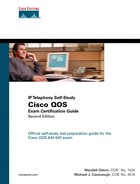
When I was a young lad in Barnesville, Georgia, I used to go to the bank with my dad. Each bank teller had his or her own line of people waiting to talk to the teller and transact their business. Invariably, we would always get behind someone who was really slow. (We called that Bubba’s law — you always get behind some large, disagreeable guy named “Bubba” in line.) So, someone who came to the bank after we did would get served before we would, because he or she didn’t get behind a “Bubba.” But, it was the rural South, so no one was in that much of a hurry, and no one really worried about it.
Later we moved to the big city of Snellville, just outside Atlanta. At the bank in Snellville, people were in a bigger hurry. So, there was one line and many tellers. As it turns out, and as queuing theory proves, the average time in the queue is decreased with one queue served by many tellers, rather than one queue for each teller. Therefore, if one slow person (Bubba) was talking to teller 1, when teller 2 became available, my dad and I could go next, rather than the person who showed up at the bank after we did. Figure 1-1 depicts the two competing queuing methods at a typical bank or fast-food chain—multiple queues, multiple servers versus single queue, multiple servers. The single queue/ multiple servers method improves average wait time, but also eliminates the possibility of your good luck in choosing a fast line—the one with no Bubbas in it.
The bank in Snellville just chose a different queuing method, and that positively affected everyone, right? Well, the choice of using a single queue did have one negative effect — because there was only one queue, you could never show up, pick one of the many queues, and happen to get in the one with only fast people in it. In this scenario, on average everyone gets better service, but you miss out on the chance to get in and out of the bank really fast. In short, most customers’ experience is improved, and some customers’ experience is degraded.
In networking, QoS describes a large array of concepts and tools that can be used to affect the packet’s access to some service. Most of us think of queuing features when we think of QoS—reordering the output queue so that one packet gets better service than another. But many other QoS features affect the quality—compression, drop policy, shaping, policing, and signaling, to name a few. In the end, whichever mechanism you use, you improve the behavior for one type of packet over another. Just like at the bank, implementing QoS is “managed fairness,” and at the same time it is “managed unfairness”—you purposefully choose to favor one packet over another. In fact, quoting Cisco’s QoS course, QoS can be defined as follows:
The ability of the network to provide better or “special” service to a set of users/applications to the detriment of other users/applications
All of us can relate to the frustration of waiting in lines (queues) for things in our daily lives. It would be great if there were never any people in line ahead of us at the tollbooths, or waiting to get on a ride at Disneyland (or any other place). For that to be possible, however, there would need to be a lot more tollbooths, Disneyland would need to be 20 times larger, and banks would need to hire a lot more tellers. Even so, adding more capacity would not always solve the problem—the tollbooth would still be crowded at rush hour, Disneyland would still be crowded when schools are not in session, and banks would still be crowded on Friday afternoons when everyone is trying to cash his or her weekly paycheck (at least where I live!). Making Disneyland 20 times larger, so that there are no queues, is financially ridiculous—likewise, the addition of 20 times more bandwidth to an existing link is probably also financially unreasonable. After all, you can afford only so much capacity, or bandwidth in the case of networking.
This chapter begins by taking a close look at the four traffic characteristics that QoS tools can affect:
![]() Bandwidth
Bandwidth
![]() Delay
Delay
![]() Jitter
Jitter
![]() Packet loss
Packet loss
Whereas QoS tools improve these characteristics for some flows, the same tools might degrade service for other flows. Therefore, before you can intelligently decide to reduce one packet’s delay by increasing another packet’s delay, you should understand what each type of application needs. The second part of this “Foundation Topics” section examines voice, video, and data flows in light of their needs for bandwidth, delay, jitter, and loss.
Different types of end-user traffic require different performance characteristics on a network. A file-transfer application might just need throughput, but the delay a single packet experiences might not matter. Interactive applications might need consistent response time. Voice calls need low, consistent delay, and video conferencing needs low, consistent delay as well as high throughput.
Users might legitimately complain about the performance of their applications, and the performance issues may be related to the network. Of course, most end users will believe the network is responsible for performance problems, whether it is or not! Reasonable complaints include the following:
![]() My application is slow.
My application is slow.
![]() My file takes too long to transfer now.
My file takes too long to transfer now.
![]() The video freezes.
The video freezes.
![]() The phone call has so much delay we keep talking at the same time, not knowing whether the other person has paused.
The phone call has so much delay we keep talking at the same time, not knowing whether the other person has paused.
![]() I keep losing calls.
I keep losing calls.
In some cases, the root problem can be removed, or at least its impact lessened, by implementing QoS features.
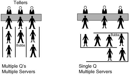
So, how do voice, video, and data traffic behave in networks that do not use QoS? Well, certainly the performance varies. Table 1-2 outlines some of the behaviors in a network without QoS.
QoS attempts to solve network traffic performance issues, although QoS is not a cure-all. To improve network performance, QoS features affect a network by manipulating the following network characteristics:
![]() Bandwidth
Bandwidth
![]() Delay
Delay
![]() Jitter (delay variation)
Jitter (delay variation)
![]() Packet loss
Packet loss
Unfortunately, improving one QoS characteristic might degrade another. Bandwidth defines the capacity of the transmission media. Compression tools reduce the amount of bandwidth needed to send all packets, but the compression process adds some delay per packet and also consumes CPU cycles. Jitter is the variation in delay between consecutive packets, so it is sometimes called “delay variation.” A router can reduce jitter for some traffic, but that usually increases delay and jitter for other traffic flows. QoS features can address jitter problems, particularly the queuing features that have priority queuing for packets that need low jitter. Packet loss can occur because of transmission errors, and QoS mechanisms cannot do much about that. However, more packets might be lost due to queues filling up rather than transmission errors—and QoS features can affect which packets are dropped.
You can think of QoS as “managed fairness” and, conversely, as “managed unfairness.” The real key to QoS success requires you to improve a QoS characteristic for a flow that needs that characteristic, while degrading that same characteristic for a flow that does not need that characteristic. For instance, QoS designs should decrease delay for delay-sensitive traffic, while increasing delay for delay-insensitive traffic.
The next four short sections take a closer look at each of these four traffic characteristics.
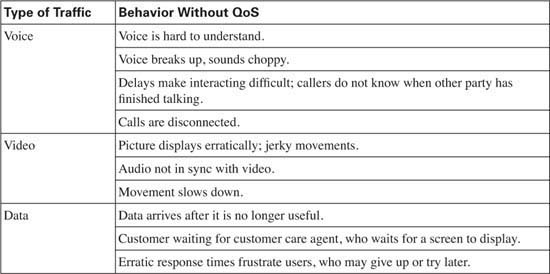
The term bandwidth refers to the number of bits per second that can reasonably be expected to be successfully delivered across some medium. In some cases, bandwidth equals the physical link speed, or the clock rate, of the interface. In other cases, bandwidth is smaller than the actual speed of the link. Consider, for example, Figure 1-2, which shows two typical networks, one with a point-to-point serial link, and the other using Frame Relay.
In the point-to-point network, WAN bandwidth equals the physical link speed, or clock rate, on the physical medium. Suppose, for instance, that the link is a 64-kbps link—you could reasonably expect to send 64 kbps worth of traffic, and expect it to get to the other side of the link. You would never expect to send more than that, because you cannot send the bits any faster than the clock rate of the interface. Bandwidth, in this case, is indeed rather obvious; you get 64 kbps in both directions.
The Frame Relay network provides a contracted amount of bandwidth. In practice, however, many installations expect more than that! The committed information rate (CIR) defines how much bandwidth the provider guarantees will pass through their network between the data terminal equipment (DTE) at each end of a virtual circuit (VC). That guarantee is a business proposition—a Layer 8 issue using the OSI reference model. On some occasions, you might not actually even get CIR worth of bandwidth. However, the Frame Relay provider commits to engineering a network so that they can support at least the CIRs of their collective VCs. In effect, bandwidth per VC equals the CIR of each VC, respectively.
Unfortunately, bandwidth on multiaccess networks is not that simple. Consider the fact that R3 has a 256-kbps access rate, and R4 has a T1 access rate. When R3 sends, it must send the bits at access rate—otherwise, Layer 1 functions would not work at all. Similarly, R4 must send at T1 speed. One of Frame Relay’s big selling points throughout its large growth years was that you “get something for nothing”—you pay for CIR of x, and you get more than x worth of bandwidth. In fact, many data network engineers design networks assuming that you will get an average of one and a half to two times CIR over each VC. If R3 and R4 send too much, and the provider’s switches have full queues, the frames are discarded, and the data has to be re-sent. If you pay for 128-kbps CIR between R3 and R4, and over time actually send at 192 kbps, or 256 kbps, and it works, how much bandwidth do you really have? Well, on a multiaccess network, such as Frame Relay or ATM, the actual amount of bandwidth is certainly open to argument.
Frame Relay bandwidth might even be less than CIR in practice. Suppose that R4 is the main site, and there are 15 remote sites identical to R3 (including R3). Can you reasonably expect to send at 128 kbps (CIR) to all 15 sites, at the same time, when R4 has a 1.544-Mbps access rate? No! All 15 sites sending at 128 kbps requires 1.920 Mbps, and R4 can only send and receive at 1.544 Mbps. Would an engineer design a network like this? Yes! The idea being that if data is being sent to all VCs simultaneously, or the Frame Relay switch will queue the data (for packets going left to right). If data is not being sent to all 15 remote sites at the same time, you get (at least) 128 kbps to each site that needs the bandwidth at that time. The negative effect is that a larger percentage of packets are dropped due to full queues; however, for data networks that is typically a reasonable tradeoff. For traffic that is not tolerant to loss, such as voice and video, this type of design may not be reasonable.
Throughout this book, when multiaccess network bandwidth is important, the discussion covers some of the implications of using the more conservative bandwidth of CIR, versus the more liberal measurements that are typically a multiple of CIR.
When you are using a Cisco router, two common interface commands relate to bandwidth. First, the clock rate command defines the actual Layer 1 bit rate. The command is used when the router is providing clocking, typically when connecting the router using a serial interface to some other nearby device (another router, for instance). The bandwidth command tells a variety of Cisco IOS Software functions how much bandwidth is assumed to be available on the interface. For instance, Enhanced Interior Gateway Routing Protocol (EIGRP) chooses metrics for interfaces based on the bandwidth command, not based on a clock rate command. In short, bandwidth only changes the behavior of other tools on an interface, and it affects the results of some statistics, but it never changes the actual rate of sending bits out an interface.
Some QoS tools refer to interface bandwidth, which is defined with the bandwidth command. Engineers should consider bandwidth defaults when enabling QoS features. On serial interfaces on Cisco routers, the default bandwidth setting is T1 speed—regardless of the actual bandwidth. If subinterfaces are used, they inherit the bandwidth setting of the corresponding physical interface. In Figure 1-2, for example, R3 would have a default bandwidth setting of 1544 (the units are in kbps), as opposed to a more accurate 128, 192, or 256 kbps, depending on how conservative or liberal the engineer can afford to be in this network.
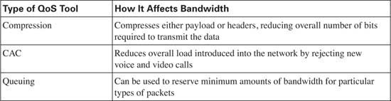
Several QoS features can help with bandwidth issues. You’ll find more detail about each of these tools in various chapters throughout this book. For now, however, knowing what each class of QoS tool accomplishes will help you sift through some of the details.
The best QoS tool for bandwidth issues is more bandwidth! However, more bandwidth does not solve all problems. In fact, in converged networks (networks with voice, video, and data), adding more bandwidth might be masking delay problems that are best solved through other QoS tools or through better QoS design. To quote Arno Penzias, former head of Bell Labs and a Nobel Prize winner: “Money and sex, storage and bandwidth: Only too much is ever enough.” If you can afford it, more bandwidth certainly helps improve traffic quality.
Some link-efficiency QoS tools improve bandwidth by reducing the number of bits required to transmit the data. Figure 1-3 shows a rather simplistic view of the effect of compression, assuming the compression ratio is 2:1. Without compression, with 80 kbps of offered traffic, and only a 64-kbps point-to-point link, a queue will form. The queue will eventually fill, and packets will be dropped off the end of the queue—an action called tail drop. With compression, if a ratio of 2:1 is achieved, the 80 kbps will require only 40 kbps in order to be sent across the link—effectively doubling the bandwidth capacity of the link.
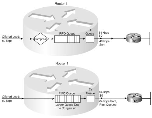
This book covers several options for compression, some of which happen before the queuing process (as shown in Figure 1-3), and some that happen after the queuing process.
The other QoS tool that directly affects bandwidth is call admission control (CAC). CAC tools decide whether the network can accept new voice and video calls. That permission might be based on a large number of factors, but several of those factors involve either a measurement of bandwidth. For example, the design might expect only three concurrent G.729A VoIP calls over a particular path; CAC would be used for each new call, and when three calls already exist, the next call would be rejected. (If CAC did not prevent the fourth call, and a link became oversubscribed as a result, all the quality of all four calls would degrade!) When CAC rejects a call, the call might be rerouted based on the VoIP dial plan, for instance, through the Public Switched Telephone Network (PSTN). (As it turns out, CAC tools are not covered in the current version of the QOS exam, 642-642.)
Queuing tools can affect the amount of bandwidth that certain types of traffic receive. Queuing tools create multiple queues, and then packets are taken from the queues based on some scheduling algorithm. The scheduling algorithm might include a feature that guarantees a minimum amount of bandwidth to a particular queue. Figure 1-4, for example, shows a two- queue system. The first queue gets 25 percent of the bandwidth on the link, and the second queue gets 75 percent of the bandwidth.

With regard to Cisco IOS Software queuing tools that reserve bandwidth, if both queues have packets waiting, the algorithm takes packets such that, over time, each queue gets its configured percentage of the link bandwidth. If only one queue has packets waiting, that queue gets more than its configured amount of bandwidth for that short period.
Although adding more bandwidth always helps, the tools summarized in Table 1-3 do help to improve the efficient utilization of bandwidth in a network.
All packets in a network experience some delay between when the packet is first sent and when it arrives at its destination. Most of the concepts behind QoS mechanisms relate in some way to delay. Therefore, a deeper look into delay is useful. Take a look at Figure 1-5; this sample network is used often in this book.

At what points will delay occur in this network? Well, at all points, in actuality. At some points in the network, the delay is so small that it can just be ignored for practical purposes. In other cases, the delay is significant, but there is nothing you can do about it! For a fuller understanding, consider the following types of delay:
![]() Serialization delay (fixed)
Serialization delay (fixed)
![]() Propagation delay (fixed)
Propagation delay (fixed)
![]() Forwarding/processing delay (variable)
Forwarding/processing delay (variable)
![]() Shaping delay (variable)
Shaping delay (variable)
![]() Network delay (variable)
Network delay (variable)
![]() Codec delay (fixed)
Codec delay (fixed)
![]() Compression delay (variable)
Compression delay (variable)
Each of these types of delay is explained over the next several pages. Together, the types of delay make up the components of the end-to-end delay experienced by a packet.
Imagine you are standing at a train station. A train comes by but doesn’t stop; it just keeps going. Because the train cars are connected serially one to another, a time lag occurs between when the engine car at the front of the train first gets to this station and when the last car passes by. If the train is long, it takes more time until the train fully passes. If the train is moving slowly, it takes longer for all the cars to pass. In networking, serialization delay is similar to the delay between the first and last cars in a train.
Serialization delay defines the time it takes to encode the bits of a packet onto the physical interface. If the link is fast, the bits can be encoded onto the link more quickly; if the link is slow, it takes longer to encode the bits on the link. Likewise, if the packet is short, it does not take as long to put the bits on the link as compared with a long packet.
Use the following formula to calculate serialization delay for a packet:
Suppose, for instance, that Hannah in Figure 1-5 sends a 125-byte packet to Server1. Hannah sends the packet over the Fast Ethernet to the switch. The 125 bytes equal 1000 bits, so at Fast Ethernet speeds, it takes 1000 bits/100,000,000 bits per second (bps), or .01 ms, to serialize the packet onto the Fast Ethernet. Another .01 ms of serialization delay is experienced when the switch sends the frame to R1. (I ignored the data-link header lengths to keep the math obvious.)
Next, when that same packet leaves R1 over a 56 kbps link to R2, serialization takes 1000 bits/ 56,000 bps, or 17.85 ms. The serialization component over Fast Ethernet is insignificant, whereas serialization becomes a more significant number on lower-speed serial links. Figure 1-6 shows the various locations where the packet from Hannah to Server1 experiences serialization delay.
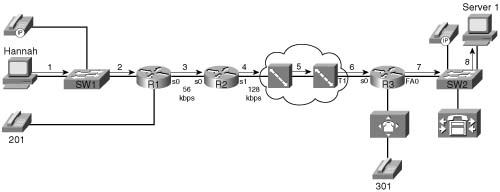
As Figure 1-6 shows, serialization delay occurs any time a frame is sent. On LAN links, the delay is insignificant for most applications. At steps 3 through 6 in the figure, the serialization delay is 17.85 ms, 7.8 ms, .02 ms, and .65 ms for the 125-byte packet, respectively. Also note that serialization delays do occur inside the Frame Relay cloud. (You can read more about delays inside the cloud in the “Network Delay” section later in this chapter.)
Table 1-4 lists the serialization delay for a couple of frame sizes and link speeds.

Imagine you are watching a train again, this time from a helicopter high in the air over the tracks. You see the train leaving one station, and then arriving at the second station. Using a stopwatch, you measure the amount of time it takes from the first car leaving the first station until the first car arrives at the second station. Of course, all the other cars take the same amount of time to get there as well. This delay is similar to propagation delay in networking.
Propagation delay defines the time it takes a single bit to get from one end of the link to the other. When an electrical or optical signal is placed onto the cable, the energy does not propagate to the other end of the cable instantaneously—some delay occurs. The speed of energy on electrical and optical interfaces approaches the speed of light, and the network engineer cannot override the laws of physics! The only variable that affects the propagation delay is the length of the link. Use the following formula to calculate propagation delay:
or
where 3.0 * 108 is the speed of light in a vacuum. Many people use 2.1 * 108 for the speed of light over copper and optical media when a more exact measurement is needed. (Seventy percent of the speed of light is the generally accepted rule for the speed of energy over electrical cabling.)
Propagation delay occurs as the bits traverse the physical link. Suppose, for instance, that the point-to-point link between R1 and R2 is 1000 kilometers (1,000,000 meters) long. The propagation delay would be as follows:
Figure 1-7 shows two contrasting examples of serialization and propagation delay.
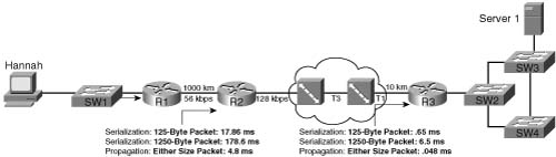
As you can see in Figure 1-7, the length of the link affects propagation delay, whereas the size of the packet and link speed affect serialization delay. The serialization delay is larger for larger packets, but the propagation delay is equal for different-sized packets, on the same link. One common misconception is that the link speed, or clock rate, affects propagation delay—it does not! Table 1-5 lists the various propagation delays and serialization delays for parts of Figure 1-6.

If the link from Hannah to SW1 is 100 meters, for example, propagation is 100/(2.1 * 108), or .48 microseconds. If the T3 between the two Frame Relay switches is 1000 kilometers, the delay is 1,000,000/(2.1 * 108), or 4.8 ms. Notice that propagation delay is not affected by clock rate on the link—even on the 56-kbps Frame Relay access link, at 1000 km (a long Frame Relay access link!), the propagation delay would only be 4.8 ms.
Packets experience queuing delay when they must wait for other packets to be sent. Most people think of queuing delay when they think of QoS, and most people think of queuing strategies and tools when they think of QoS tools—but queuing tools are just one category of QoS tool. Queuing delay consists of the time spent in the queues inside the device—typically just in output queues in a router, because input queuing is typically negligible in a router. However, the queuing time can be relatively large—hundreds of milliseconds, or maybe even more. Consider Figure 1-8, where R1 queues four 1500-byte packets that Hannah sent to Server1.

Because it takes 1500 * 8 / 56,000, or 214 ms, to serialize each 1500-byte packet, the other packets need to either be stored in memory or discarded. Therefore, the router uses some memory to hold the packets. The simplest form of queuing is to use a single queue, serviced with first-in, first-out (FIFO) logic—as is shown in the figure. After 856 ms, all four packets would have been sent out the serial link. Assuming that the link was not busy when Hannah sent these four packets, how much queuing delay did each packet experience? Well, the first packet experienced no queuing delay. The second packet waited on the first, or 214 ms. The third packet waited on the first two—or 428 ms. And the fourth packet waited on the first three, for a total of 642 ms.
Queuing provides a useful function, because the second, third, and fourth packets would have had to have been discarded without queuing. However, too much of a good thing is not always good! Imagine that Hannah sends 100 * 1500-byte packets all at once. If the queue in R1 is large enough, R1 could queue all 100 packets. What would the delay be for the one-hundredth packet? Well, 99 * 214 ms per packet, or roughly 21 seconds! If Hannah uses TCP, then TCP has probably timed out, and re-sent the packets—causing more congestion and queuing delay. And what about another user’s packet that showed up right after Hannah’s 100 packets? Still more delay. So, some queuing helps prevent packet drops, but large queues can cause too much delay.
Figure 1-9 combines all the delay components covered so far into one small diagram. Consider the delay for the fourth of the four 1500-byte packets sent by Hannah. The figure lists the queuing, serialization, and propagation delays.

The overall delay for a packet is the sum of all these delays from end to end. At R1, when all four packets have been received, the fourth packet experiences a total of about 860 ms of delay before it has been fully received at R2. And this example just shows the queuing delay in a single router (R1), and the serialization and propagation delay over a single link—end-to-end delay includes these delays at each router (queuing) and link (serialization and propagation) in the network.
The term forwarding delay refers the processing time between when a frame is fully-received, and when the packet has been placed in an output queue. So, forwarding delay does not include the time the packet sits in the output queue waiting to leave the router. It does include the time required for the router to process the route, or forward, the packet.
Cisco does not normally quote statistics about forwarding delay numbers for different models of routers with different types of internal processing. However, the higher volume of packets that a router can forward, and the higher volume of packets forwarded using a particular processing method, presumably the lower the forwarding delay.
Most delay components in LAN switches are small enough not to matter. However, switches incur forwarding delay, just like routers—most of the time. Some LAN switches use a “store- and- forward” forwarding logic, when the entire frame must be received before forwarding any part of the frame. However, some switches use cut-through or fragment-free forwarding, which means that the first bits of a frame are forwarded before the final bits are fully received. Technically, if you define forwarding delay as the time between receipt of the entire frame until that frame is queued for transmission, some LAN switches might actually have negative forwarding delay! It just depends on how you decide to define what parts of the overall delay end up being attributed. Forwarding delay is typically a small enough component to ignore in overall delay budget calculations, so this book does not punish you with further discussion about these details!
For more information on internal processing methods such as Cisco Express Forwarding (CEF), you can review the Cisco Press book Inside Cisco IOS Software Architecture.
Traffic shaping causes additional delays by serving queues more slowly than if traffic shaping were not used. Why should a router slow down sending packets if it does not have to? Well, traffic shaping helps match the overall forwarding rate of traffic when a carrier might discard traffic if the rates exceed the contracted rate. So, which is better?
![]() Sending packets really fast and having them be dropped
Sending packets really fast and having them be dropped
![]() Sending packets more slowly, but not having them be dropped
Sending packets more slowly, but not having them be dropped
The right answer is—it depends! If you want to send more slowly, hoping that packets are not dropped, however, traffic shaping is the solution.
Carriers can drop frames and packets inside their network for a variety of reasons. One of the most typical reasons is that most central-site routers use a fast access link, with remote sites using much slower links. If the central site uses a T1, and the remote site uses a 56-kbps link, frames may fill the queue inside the service provider’s network, waiting to go across the 56-kbps access link. Many other events can cause the carrier to drop packets; these reasons events explained more fully in Chapter 6, “Traffic Policing and Shaping.”
To understand the basic ideas behind shaping in a single router, consider Figure 1-10, where R2 has a 128-kbps access rate and a 64-kbps CIR on its VC to R3.

Suppose that the Frame Relay provider agrees to the 64-kbps CIR on the VC from R2 to R3, but the carrier tells you that they aggressively discard frames when you send more than 64 kbps. The access rate is 128 kbps. Therefore, you decide to shape, which means that R2 will want to average sending at 64 kbps, because sending faster than 64 kbps hurts more than it helps. In fact, in this particular instance, if R2 sends packets for this VC only half the time, the rate averages out to 64 kbps. Remember, bits can only be sent at the physical link speed, which is also called the access rate in Frame Relay. In effect, the router sends all packets at access rate, but the router purposefully delays sending packets, possibly even leaving the link idle, so that the rate over time averages to be about 64 kbps.
Chapter 6 will clear up the details. The key concept to keep in mind when reading other sections of this book is that traffic shaping introduces additional delay. Like many QoS features, shaping attempts to enhance one particular traffic characteristic (drops), but must sacrifice another traffic characteristic (delay) to do so.
Most people draw a big cloud for a Frame Relay or ATM network, because the details are not typically divulged to the customer. However, the same types of delay components seen outside the cloud also exist inside the cloud—and the engineer that owns the routers and switches outside the cloud cannot exercise as much QoS control over the behavior of the devices in the cloud.
So how much delay should a packet experience in the cloud? Well, it will vary. The carrier might commit to a maximum delay value as well. However, with a little insight, you can get a solid understanding of the minimum delay a packet should experience through a Frame Relay cloud. Consider Figure 1-11, focusing on the Frame Relay components.
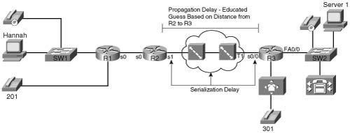
The propagation delay and serialization delay can be guessed pretty closely. No matter how many switches exist between R2 and R3, the cumulative propagation delays on all the links between R2 and R3 will be at least as much as the propagation delay on a point-to-point circuit. And with most large providers, because they have many points of presence (PoPs), the Frame Relay VC probably takes the same physical route as a point-to-point circuit would anyway. As for serialization delay, the two slowest links, by far, will be the two access links (in most cases). Therefore, the following account for most of the serialization delay in the cloud:
![]() The serialization delay to send the packet into the cloud
The serialization delay to send the packet into the cloud
![]() The serialization delay at the egress Frame Relay switch, sending the packet to R3
The serialization delay at the egress Frame Relay switch, sending the packet to R3
Suppose, for example, that R2 and R3 are 1000 km apart, and a 1500-byte packet is sent. The network delay will at least be the propagation delay plus both serialization delays on the two access links:
Propagation = 1000 km / 2.1 * 108 = 4.8 ms
Serialization (ingress R2) = 1500 bytes * 8 / 128,000 bps = 94 ms
Serialization (egress R3) = 1500 bytes * 8 / 1,544,000 = 7.8 ms
For a total of 106.6 ms delay
Of course, the delay will vary—and will depend on the provider, the status of the network’s links, and overall network congestion. In some cases, the provider will include delay limits in the contracted service-level agreement (SLA).
Queuing delay inside the cloud creates the most variability in network delay, just as it does outside the cloud. These delays are traffic dependent, and hard to predict.
Of the types of delay covered so far in this chapter, all except shaping delay occur in every network. Shaping delay occurs only when shaping is enabled.
Two other delay components may or may not be found in a typical network. First, codec delay will be experienced by voice and video traffic. Codec delay is covered in more depth in the section titled “Voice Delay Considerations” later in this chapter. Compression requires processing, and the time taken to process a packet to compress or decompress the packet introduces delay. Chapter 8, “Link-Efficiency Tools,” covers compression delay.
Table 1-6 summarizes the delay components listed in this section.

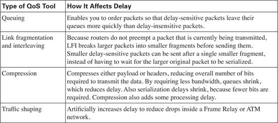
Several QoS features can help with delay issues. You’ll find more detail about each of these tools in various chapters throughout this book. For now, however, knowing what each class of QoS tool accomplishes will help you sift through some of the details.
The best QoS tool for delay issues is . . . more bandwidth—again! More bandwidth helps bandwidth-related problems, and it also helps delay-related problems. Faster bandwidth decreases serialization delay. Because packets exit more quickly, queuing delay decreases. Higher CIR on your VCs reduces shaping delay. In short, faster bandwidth reduces delay!
Unfortunately, more bandwidth does not solve all delay problems, even if you could afford more bandwidth! In fact, in converged networks (networks with voice, video, and data), adding more bandwidth might mask delay problems that are best solved through other QoS tools or through better QoS design. The sections that follow address the QoS tools can affect the delay a particular packet receives.
The most popular QoS tool, queuing, involves choosing the packets to be sent based on something other than arrival time. In other words, instead of FIFO queuing with one queue, other queuing mechanisms create multiple queues, place packets into these different queues, and then pick packets from the various queues. As a result, some packets leave the router more quickly, with other packets having to wait longer. Although queuing does not decrease delay for all packets, it can decrease delay for delay-sensitive packets, and increase delay for delay-insensitive packets—and enabling a queuing mechanism on a router does not cost any cash, whereas adding more bandwidth does.
Each queuing method defines some number of different queues, with different methods of scheduling the queues—in other words, different rules for how to choose from which queue the next packet to be sent will be chosen. Figure 1-12 depicts a queuing mechanism with two queues. Suppose Hannah sent four packets, but the fourth packet was sent by a video- conferencing package she was running, whereas the other three packets were for a web application she was using while bored with the video conference.

R1 could notice that packet 4 has different characteristics, and place it into a different queue. Packet 4 could exit R1 before some or all of the first three packets.
The time required to serialize a packet on a link is a function of the speed of the link, and the size of the packet. When the router decides to start sending the first bit of a packet, the router continues until the whole packet is sent. Therefore, if a delay-sensitive packet shows up just after a long packet has begun to be sent out an interface, the delay-sensitive packet must wait until the longer packet has been sent.
Suppose, for example, that two packets have arrived at R1. Packet 1 is 1500 bytes, and packet 2 is 200 bytes. The smaller packet is delay sensitive. Because packet 2 arrived just after the first bit of packet 1 was sent, packet 2 must wait 214 ms for packet 1 to be serialized onto the link. With link fragmentation and interleaving (LFI), packet 1 could be broken into three 500-byte fragments, and packet 2 could be interleaved (inserted) and sent on the link after the first of the three fragments of packet 1. Figure 1-13 depicts LFI operation.

Note that packet 1 was fragmented into three pieces. Because packet 2 arrived after packet 1 had begun to be sent, packet 2 had to wait. With LFI, packet 2 does not have to wait for the entire original packet, but rather it waits for just 1 fragment to be sent.
Compression takes a packet, or packet header, and compresses the data so that it uses fewer bits. Therefore, a 1500-byte packet, compressed to 750 bytes, takes half as much serialization time as does an uncompressed 1500-byte packet.
Compression reduces serialization delay, because the number of bits used to send a packet is decreased. However, delay may also be increased because of the processing time required to compress and decompress the packets. Chapter 8, “Link Efficiency Tools,” covers the pros and cons of each type of compression.
Consecutive packets that experience different amounts of delay have experienced jitter. In a packet network, with variable delay components, jitter always occurs—the question is whether the jitter impacts the application enough to degrade the service. Typically, data applications expect some jitter, and do not degrade. However, some traffic, such as digitized voice, requires that the packets be transmitted in a consistent, uniform manner (for instance, every 20 ms). The packets should also arrive at the destination with the same spacing between them. (This type of traffic is called isochronous traffic.)
Jitter is defined as a variation in the arrival rate (that is, variation in delay through the network) of packets that were transmitted in a uniform manner. Figure 1-14, for example, shows three packets as part of a voice call between phones at extension 301 and 201.

The phone sends the packets every 20 ms. Notice that the second packet arrived 20 ms after the first, so no jitter occurred. However, the third packet arrived 30 ms after the second packet, so 10 ms of jitter occurred.
Voice and video degrade quickly when jitter occurs. Data applications tend to be much more tolerant of jitter, although large variations in jitter affect interactive applications.
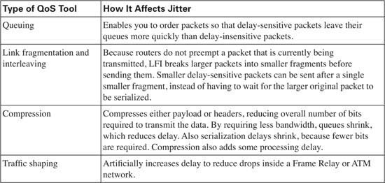
Several QoS features can help with jitter issues. You’ll find more detail about each of these tools in various chapters throughout this book. For now, however, knowing what each class of QoS tool accomplishes will help you sift through some of the details.
The best QoS tool for jitter issues is . . . more bandwidth—again! More bandwidth helps bandwidth-related problems, and it also helps delay-related problems. If it helps to reduce delay, and because jitter is the variation of delay, jitter will be smaller. Faster bandwidth decreases serialization delay, which will decrease jitter. For instance, if delay has been averaging between 100 ms and 200 ms, jitter would typically be up to 100 ms. If delay is reduced to between 50 ms and 100 ms by adding more bandwidth, the typical jitter can be reduced to 50 ms. Because packets exit more quickly, queuing delay decreases. If queuing delays had been between 50 and 100 ms, and now they are between 10 and 20 ms, jitter will shrink as well. In short, faster is better for bandwidth, delay, and jitter issues!
Unfortunately, more bandwidth does not solve all jitter problems, even if you could afford more bandwidth! Several classes of QoS tools improve jitter; as usual, decreasing jitter for one set of packets increases jitter for others.
The same set of tools that affect delay also affect jitter; refer to Table 1-8 for a brief list of these QoS tools.
The last QoS traffic characteristic is packet loss, or just loss. Routers lose/drop/discard packets for many reasons, most of which QoS tools can do nothing about. For instance, frames that fail the incoming frame check sequence (FCS) are discarded—period. However, QoS tools can be used to minimize the impact of packets lost due to full queues.
In most networks today, the number of packets lost due to bit errors is small, typically less than one in one billion (bit error rate [BER] of 10−9 or better). Therefore, the larger concern for packet loss is loss due to full buffers and queues. Consider Figure 1-15, with Hannah sending 50 consecutive 1500-byte packets, and R1 having a queue of size 40.
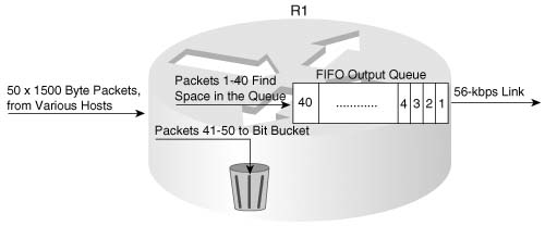
The term “tail drop” refers to when a router drops a packet when it wants to put the packet at the end or the tail of the queue. As Figure 1-15 shows, when all 40 queue slots are filled, the rest of the 50 packets are dropped. In a real network, a few of the packets might be sent out the serial link before all 50 packets are received, so maybe not all 10 packets are lost, but certainly a large number of packets would be lost.
Some flows tolerate loss better than others do. For instance, the human ear can detect loss of only 10 ms of voice, but the listener can generally understand speech with such small loss. Cisco digital signal processors (DSPs) can predict the contents of lost voice packets, up to 30 ms when using the G.729 codec. By default, each voice packet contains 20 ms of voice; so if two consecutive voice packets are lost, the DSP cannot re-create the voice, and the receiver can actually perceive the silence. Conversely, web traffic tolerates loss well, using TCP to recover the data.
Only a few QoS features can help with packet loss issues. You’ll find more detail about each of these tools in various chapters throughout this book. For now, however, knowing what each class of QoS tool accomplishes will help you sift through some of the details.
By now, you should guess that bandwidth will help prevent lost packets. More bandwidth helps—it just does not solve all problems. And frankly, if all you do is add more bandwidth, and you have a converged voice/video/data network, you will still have quality issues.
How does more bandwidth reduce loss? More bandwidth allows packets to be transmitted faster, which reduces the length of queues. With shorter queues, the queues are less likely to fill. Unless queues fill, packets are not tail dropped.
You can use one class of tool to help reduce the impacts of loss. This class is called Random Early Detection.
TCP uses a windowing protocol, which restricts the amount of data a TCP sender can send without an acknowledgment. Each TCP window for each different TCP connection grows and shrinks based on many factors. RED works under the assumption that if some of the TCP connections can be made to shrink their windows before output queues fill, the collective number of packets sent into the network will be smaller, and the queue will not fill. During times when the queues are not getting very full, RED does not bother telling the TCP senders to slow down, because there is no need to slow down.
RED just discards some packets before a queue gets full and starts to tail drop. You can almost think of RED tools as managing the end of a queue, while the queuing tool manages the front of the queue! Because most traffic is TCP based and TCP slows down sending packets after a earlier packet is lost, RED reduces the load of packets that are entering the network before the queues fill. RED requires a fairly detailed explanation for a true understanding of what it does, and how it works. However, the general idea can be easily understood, as long as you know that TCP will slow down sending, by reducing its window size, when packets are lost.
TCP uses a window, which defines how much data can be sent before an acknowledgment is received. The window changes size dynamically, based on several factors, including lost packets. When packets are lost, depending on other conditions, a TCP window shrinks to 50 percent of the previous window size. With most data traffic being TCP in a typical network, when a large amount of tail drop occurs, almost all, if not all TCP connections sending packets across that link have their TCP windows shrunk by 50 percent at least once.
Consider the example in Figure 1-15. As that figure shows, 50 packets were sent, and the queue filled, and 10 of those packets were lost. If those 50 packets were part of 10 different TCP connections, and all 10 connections lost packets in the big tail drop, the next time the hosts send, only 25 total packets would be sent (windows all cut in half).
With RED, before tail drop occurs, RED discards some packets, forcing only a few of the TCP connections to slow down. By allowing only a few of the TCP windows to be reduced, tail drops can be avoided, and most users get better response time. The collective TCP sending rate stabilizes to a level for which tail drops seldom if ever occur. For those TCP connections for which RED dropped packets, response time is temporarily slow. However, that is much better than all users experiencing slow response time!
Queuing accomplishes a lot of tasks—including reducing loss. Because loss occurs when queues fill, and because the queuing methods typically provide the ability to configure the maximum queue size, you can just make the queue longer. With a longer maximum queue size, likelihood of loss decreases. However, queuing delay increases. Consider, for instance, Figure 1-16.

In the top example, a single FIFO queue is used. For delay-sensitive traffic, waiting behind 49 other packets might not work well. For applications that are loss sensitive, but not as delay sensitive, however, a long queue might work better. One goal might be to put delay-sensitive traffic into a different queue from loss-sensitive traffic, with an extra-long queue length for the loss-sensitive traffic, as shown in the bottom part of the figure. As usual, a tradeoff occurs—in this case, between low loss and low delay.
Table 1-9 summarizes the points concerning the two types of QoS tools that affect loss.

This book covers a wide variety of QoS tools, and every tool either directly or indirectly affects bandwidth, delay, jitter, or loss. Some tools improve a QoS characteristic for one packet, but degrade it for others. For example, queuing tools might let one packet go earlier, reducing delay, while increasing delay for other packets. Some QoS tools directly impact one characteristic, but indirectly affect others. For instance, RED manages loss directly, but it indirectly reduces delay for some flows because RED generally causes queue sizes to decrease.
As this book explains each new feature in detail, you will also find a summary of how the feature manages bandwidth, delay, jitter, and loss.
So why do you need QoS? QoS can affect a network’s bandwidth, delay, jitter, and packet loss properties. Applications have different requirements for bandwidth, delay, jitter, and packet loss. With QoS, a network can better provide the right amounts of QoS resources for each application.
The next three sections cover voice, video, and data flows. Earlier versions of the QOS exam included more coverage of the QoS characteristics of voice, video, and data; however, the current QoS exam does not cover these topics in as much depth. Many readers of the previous edition of this book let us know that the following sections provided a lot of good background information, so, it’s probably worth reading through the details in the rest of this chapter, but more of the focus on the QOS exam will come from the remaining chapters in this book. If you choose to skip over this section, make sure to catch the short section titled “Planning and Implementing QoS Policies” near the end of this chapter’s “Foundation Topics” Section.
Voice traffic can degrade quickly in networks without QoS tools. This section explains enough about voice traffic flows to enable the typical reader to understand how each of the QoS tools applies to voice.
Note This book does not cover voice in depth because the details are not directly related to QoS. For additional information, refer to the following sources:
Deploying Cisco Voice over IP Solutions, Cisco Press, Davidson and Fox
IP Telephony, Hewlett-Packard Professional Books, Douskalis
Voice over IP Fundamentals, Cisco Press, Davidson and Peters
IP Telephony, McGraw Hill, Goralski and Kolon
Without QoS, the listener experiences a bad call. The voice becomes choppy or unintelligible. Delays can cause poor interactivity—for instance, the two callers keep starting to talk at the same time, because the delays sound like the other person speaking has finished what he or she had to say. Speech is lost, so that there is a gap in the sound that is heard. Calls might even be disconnected.
Most QoS issues can be broken into an analysis of the four QoS characteristics: bandwidth, delay, jitter, and loss. The basics of voice over data networks is covered first, followed by QoS details unique to voice in terms of the four QoS characteristics.
Voice over data includes Voice over IP (VoIP), Voice over Frame Relay (VoFR), and Voice over ATM (VoATM). Each of these three voice over data technologies transports voice, and each is slightly different. Most of the questions you should see on an exam will be related to VoIP, and not VoFR or VoATM, because of the three options, VoIP is the most pervasive. Also calls between Cisco IP Phones use VoIP, not VoFR or VoATM.
Imagine a call between the two analog phones in Figure 1-17, extensions 201 and 301.
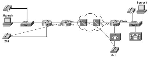
Before the voice can be heard at the other end of the call, several things must happen. Either user must pick up the phone and dial the digits. The router connected to the phone interprets the digits and uses signaling to set up the VoIP call. (Because both phones are plugged into FXS analog ports on R1 and R3, the routers use H.323 signaling.) At various points in the signaling process, the caller hears ringing, and the called party hears the phone ringing. The called party picks up the phone, and call setup is complete.
The actual voice call (as opposed to signaling) uses Real-Time Transport Protocol (RTP). Figure 1-18 outlines the format of an IP packet using RTP.
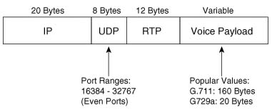
In the call between the two analog phones, the router collects the analog voice, digitizes the voice, encodes the voice using a voice codec, and places the encoded voice into the payload field shown in Figure 1-18. For instance, R1 would create an IP packet as shown in Figure 1-18, place the encoded voice bits into the voice payload field, and send the packet. The source IP address would be an IP address on R1, and the destination IP address would be an IP address on R3. When R3 receives the packet, it reverses the process, eventually playing the analog waveform for the voice out to the analog phone.
The IP Phones would experience a similar process in concept, although the details differ. The signaling process includes the use of Skinny Station Control Protocol (SSCP), with flows between each phone and the Cisco CallManager server. After signaling has completed, an RTP flow has been completed between the two phones. CallManager does not participate directly in the actual call, but only in call setup and teardown. (CallManager does maintain a TCP connection to each phone for control function support.) R1 and R3 do not play a role in the creation of the RTP packets on behalf of the IP Phone, because the IP Phones themselves create the packets. As far as R1 and R3 are concerned, the packets sent by the IP Phones are just IP packets.
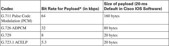
Finally, the network administrator can choose from various coders/decoders (codecs) for the VoIP calls. Codecs process the incoming analog signal and convert the signal into a digital (binary) signal. The actual binary values used to represent the voice vary based on which codec is used. Each codec has various features, the most significant feature being the amount of bandwidth required to send the voice payload created by the codec. Table 1-10 lists the most popular codecs, and the bandwidth required for each.
This short section on voice basics (and yes, it is very basic!) can be summarized as follows:
![]() Various voice signaling protocols establish an RTP stream between the two phones, in response to the caller pressing digits on the phone.
Various voice signaling protocols establish an RTP stream between the two phones, in response to the caller pressing digits on the phone.
![]() RTP streams transmit voice between the two phones (or between their VoIP gateways).
RTP streams transmit voice between the two phones (or between their VoIP gateways).
Why the relatively simple description of voice? All voice payload flows need the same QoS characteristics, and all voice signaling flows collectively need another set of QoS characteristics. While covering each QoS tool, this book suggests how to apply the tool to “voice”—for two subcategories, namely voice payload (RTP packets) and voice signaling. Table 1-11 contrasts the QoS requirements of voice payload and signaling flows.
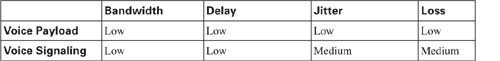
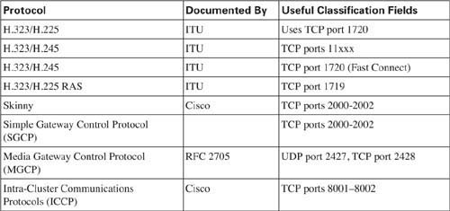
QoS tools can treat voice payload differently than they treat voice signaling. To do so, each QoS tool first classifies voice packets into one of these two categories. To classify, the QoS tool needs to be able to refer to a field in the packet that signifies that the packet is voice payload, voice signaling, or some other type of packet. Table 1-12 lists the various protocols used for signaling and for voice payload, defining documents, and identifying information.

The next few sections of this book examine voice more closely in relation to the four QoS characteristics: bandwidth, delay, jitter, and loss.
Voice calls create a flow with a fixed data rate, with equally spaced packets. Voice flows can be described as isochronous, which, according to Dictionary.com, means “characterized by or occurring at equal intervals of time.” Consider Figure 1-19, where a call has been placed between analog phones at extensions 201 and 301.

R1 creates the IP/UDP/RTP voice payload packets and sends them, by default, every 20 ms. Because Cisco IOS Software places 20 ms of encoded voice into each packet, a packet must be sent every 20 ms. So, how much bandwidth is really needed for the voice payload call? Well, actual bandwidth depends on several factors:
![]() Codec
Codec
![]() Packet overhead (IP/UDP/RTP)
Packet overhead (IP/UDP/RTP)
![]() Data-link framing (depends on data links used)
Data-link framing (depends on data links used)
![]() Compression
Compression
Most people quote a G.711 call as taking 64 kbps, and a G.729 call as taking 8 kbps. Those bandwidth numbers consider the payload only—ignoring data-link, IP, UDP, and RTP headers.
The bandwidth requirements vary dramatically based on the codec and the compression effect if RTP header compression is used. Compressed RTP (cRTP) actually compresses the IP/UDP/ RTP headers, with dramatic reduction in bandwidth when used with lower bit-rate codecs. With G.711, because a large percentage of the bandwidth carries the payload, cRTP helps, but the percentage decrease in bandwidth is not as dramatic. In either case, cRTP can increase delay caused while the processor compresses and decompresses the headers.
Note Although other codecs are available, this book compares G.711 and G.729 in most examples, noting any conditions where a different specific codec may need different treatment with QoS.
ATM can add a significant amount of data-link overhead to voice packets. Each ATM cell has 5 bytes of overhead; in addition, the last cell holding parts of the voice packet may have a lot of wasted space. For instance, a voice call using G.729 will have a packet size of 60 bytes. ATM adds about 8 bytes of framing overhead, and then segments the 68-byte frame into two cells— one using the full 48 bytes of ATM cell payload, and the other only using 20 bytes of the cell payload area—with 28 bytes “wasted.” Therefore, to send one voice “packet” of 60 bytes, two cells, in total 106 bytes, must be sent over ATM. One option to lessen the overhead is to change the payload size to contain 30 ms of voice with a G.729 codec—which interestingly also only takes two ATM cells.
Voice Activity Detection (VAD) also affects the actual bandwidth used for a voice payload call. VAD causes the sender of the voice packets to not send packets when the speaker is silent. Because human speech is typically interactive (I know there are some exceptions to that rule that come to mind right now!), VAD can decrease the actual bandwidth by about 60 percent. The actual amount of bandwidth savings for each call cannot be predicted—simple things such as calling from a noisy environment defeats VAD. Also VAD can be irritating to listeners. After a period of not speaking, the speaker starts to talk. The VAD logic may perform front-end speech clipping, which means that the first few milliseconds of voice are not sent.
Table 1-13 shows a side-by-side comparison of the actual bit rates used for two codecs and a variety of data link protocols. This table also shows rows when using the most popular codec’s default of 20 ms of voice payload (50 packets per second) for a voice call, versus 30 ms of voice payload per packet (33.3 packets per second).

* Layer 3 bandwidth consumption refers to the amount of bandwidth consumed by the Layer 3 header through the data (payload) portion of the packet.
One of the more interesting facts about the numbers in this table is that G.729 over ATM has a significant advantage when changing from 50 pps (20 ms of payload per packet) to 33 pps (30 ms of payload per packet). That’s because you need 2 ATM cells to forward a 60-byte VoIP packet (20 ms payload of G.729), and you also need two cells to forward an 80-byte VoIP packet (30 ms payload of G.729).
Voice call quality suffers when too much delay occurs. The symptoms include choppy voice, and even dropped calls. Interactivity also becomes difficult—ever had a call on a wireless phone, when you felt like you were talking on a radio? “Hey Fred, let’s go bowling—OVER”— “Okay, Barney, let’s go while Betty and Wilma are out shopping—OVER.” With large delays, it sometimes becomes difficult to know when it is your turn to talk.
Voice traffic experiences delays just like any other packet, and that delay originates from several other sources. For a quick review on delay components covered so far, consider the delay components listed in Table 1-14.

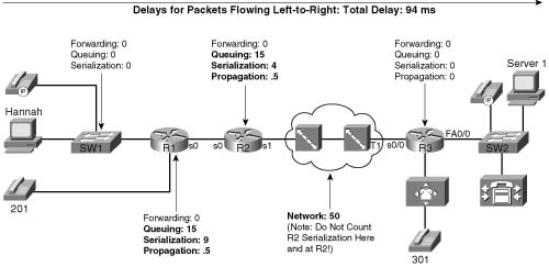
Figure 1-20 shows an example of delay concepts, with sample delay values shown. When the delay is negligible, the delay is just listed as zero. The figure lists sample delay values. The values were all made up, but with some basis in reality. Forwarding delays are typically measured in microseconds, and become negligible. The propagation delay from R1 to R2 is calculated based on a 100-km link. The serialization delays shown were calculated for a G.729 call’s packet, no compression, assuming PPP as the data- link protocol. The queuing delay varies greatly; the example value of 15 ms on R1’s 56-kbps link was based on assuming a single 105-byte frame was enqueued ahead of the packet whose delay we are tracking—which is not a lot of queuing delay. The network delay of 50 ms was made up—but that is a very reasonable number. The total delay is only 94 ms—to data network engineers, the delay seems pretty good.
So is this good enough? How little delay does the voice call tolerate? The ITU defines what it claims to be a reasonable one-way delay budget. Cisco has a slightly different opinion. You also may have applications where the user tolerates large delays to save cash. Instead of paying $3 per minute for a quality call to a foreign country, for instance, you might be willing to tolerate poor quality if the call is free. Table 1-15 outlines the suggested delay budgets.

With the example in Figure 1-20, the voice call’s delay fits inside the G.114 recommended delay budget. However, voice traffic introduces a few additional delay components, in addition to the delay factors that all data packets experience:
![]() Codec delay
Codec delay
![]() Packetization delay
Packetization delay
![]() De-jitter buffer delay (initial playout delay)
De-jitter buffer delay (initial playout delay)
Be warned—many books and websites use different terms to refer to the component parts of these three voice-specific types of delay. The terms used in this book are consistent with the Cisco courses, and therefore with the exams.
Codec delay and packetization delay coincide with each other. To get the key concepts of both, consider Figure 1-21, which asks the question, “How much delay happens between when the human speaks, and when the IP packets are sent?”
Figure 1-21 Codec and Packetization Delays Between the Instant the Speaker Speaks and When the Packet Holding the Speech Is Sent

Consider what has to happen at the IP Phones before a packet can be sent. The caller dials digits, and the call is set up. When the call is set up, the IP Phone starts sending RTP packets. When these packets begin, they are sent every 20 ms (default)—in other words, each packet has 20 ms of voice inside the voice payload part of the packet. But how much time passes between when the speaker makes some sound and when the voice packet containing that sound is first sent?
Consider sounds waves for an instant. If you and I sit in the same room and talk, the delay from when you speak and when I hear it is very small, because your voice travels at the speed of sound, which is roughly 1000 km per hour. With packet telephony, the device that converts from sound to analog electrical signals, then to digital electrical signals, and then puts that digital signal (payload) into a packet, needs time to do the work. So there will be some delay between when the speaker speaks and when the IP/UDP/RTP payload packet is sent. In between when the speaker talks and when a packet is sent, the following delays are experienced:
![]() Packetization delay
Packetization delay
![]() Codec delay
Codec delay
The IP Phone or voice gateway must collect 20 ms of voice before it can put 20 ms worth of voice payload into a packet. (The defaults for G.711 and G.729 on IP Phones and Cisco IOS Software gateways are to put 20 ms of voice into an RTP packet; the value can be changed.) Therefore, for the sake of discussion in this book, we consistently consider packet delay always to be 20 ms in examples. That is, the speaker must talk for 20 ms before a packet containing 20 ms of voice can be created.
Codec delay has two components:
![]() The time required to process an incoming analog signal and convert it to the correct digital equivalent
The time required to process an incoming analog signal and convert it to the correct digital equivalent
![]() A feature called look-ahead
A feature called look-ahead
With the first component of codec delay, which is true for all codecs, the IP Phone or gateway must process the incoming analog voice signal and encode the digital equivalent based on the codec in use. For instance, G.729 processes 10 ms of analog voice at a time. That processing does take time—in fact, the actual conversion into G.729 CS-ACELP (Conjugate Structure Algebraic Code Excited Linear Predictive) takes around 5 ms. Some documents from Cisco cite numbers between 2.5 and 10 ms, based on codec load.
The codec algorithm may cause additional delays due to a feature called look-ahead. Look- ahead occurs when the codec is predictive—in other words, one method of using fewer bits to encode voice takes advantage of the fact that the human vocal cords cannot instantaneously change from one sound to a very different sound. By examining the voice speech, and knowing that the next few ms of sound cannot be significantly different, the algorithm can use fewer bits to encode the voice—which is one way to improve from 64-kbps G.711 to an 8-kbps G.729 call. However, a predictive algorithm typically requires the codec to process some voice signal that will be encoded, plus the next several milliseconds of voice. With G.729, for example, to process a 10-ms voice sample, the codec must have all of that 10 ms of voice, plus the next 5 ms, in order to process the predictive part of the codec algorithm.
So, the G.729a codec delays the voice as follows, for each 10-ms sample, starting with the time that the 10 ms to be encoded has arrived:
5 ms look-ahead + 5 ms processing (average) = 10 ms
Remember, codec delay is variable based on codec load. The white paper, “Understanding Delay in Packet Voice Networks,” at Cisco.com provides more information about this topic (www.cisco.com/warp/public/788/voip/delay-details.html).
You need to consider packetization delay and codec delay together, because they do overlap. For instance, packetization delay consumes 20 ms while waiting on 20 ms of voice to occur. But what else happens in the first 20 ms? Consider Table 1-16, with a timeline of what happens, beginning with the first uttered sound in the voice call.

Notice that the packetization and codec delays overlap. Although each takes 20 ms, because there is overlap, the packet actually experiences about 30 ms of total delay instead of a total of 40 ms.
De-jitter buffer delay is the third voice delay component. Jitter happens in data networks. You can control it, and minimize it for jitter-sensitive traffic, but you cannot eliminate it. Buy why talk about jitter in the section on delay? Because a key tool in defeating the effects of jitter, the de-jitter buffer (sometimes called the jitter buffer) actually increases delay.
The de-jitter buffer collects voice packets and delays playing out the voice to the listener, to have several ms of voice waiting to be played. By doing so, if the next packet experiences jitter and shows up late, the de-jitter buffer’s packets can be played out isochronously, so the voice sounds good. This is the same tool used in your CD player in your car—the CD reads ahead several seconds, knowing that your car will hit bumps, knowing that the CD temporarily will not be readable—but having some of the music in solid-state memory lets the player continue to play the music. Similarly, the de-jitter buffers “reads ahead” by collecting some voice before beginning playout, so that delayed packets are less likely to cause a break in the voice.
The de-jitter buffer must be filled before playout can begin. That delay is called the initial playout delay and is depicted in Figure 1-22.
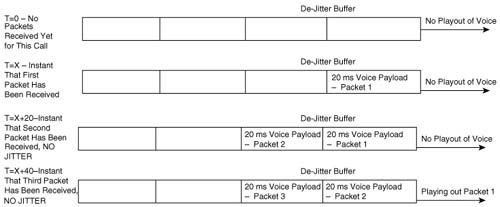
In this figure, the de-jitter buffer shows the initial playout delay. The time difference between when the initial packet arrives, and when the third packet arrives, in this particular case, is 40 ms. (Cisco IOS gateways default to 40 ms of initial playout delay.) In fact, if the initial playout delay were configured for 40 ms, this delay would be 40 ms, regardless of when the next several packets arrive. Consider, for instance, Figure 1-23, which gives a little insight into the operation of the de-jitter buffer.

In Figure 1-23, the playout begins at the statically set playout delay interval—40 ms in this case—regardless of the arrival time of other packets. A 40-ms de-jitter playout delay allows jitter to occur—because we all know that jitter happens—so that the played-out voice can continue at a constant rate.
Figure 1-24 summarizes all the delay components for a voice call. This figure repeats the same example delay values as did Figure 1-20, but with voice-specific delays added for codec, packetization, and de-jitter delays shown.

The delay has crept beyond the acceptable limits of one-way delay, according to G.114, but slightly under the limit of 200 ms suggested by Cisco. Without the additional voice delays, the 150-ms delay budget seemed attainable. With 30 ms of codec and packetization delay, however, and a (reasonable) default of 40-ms de-jitter delay (actually, de-jitter initial playout delay), 70 ms of that 150/200-ms delay is consumed. So, what can you do to stay within the desired delay budget? You attack the variable components of delay. Table 1-17 lists the different delay components, and whether they are variable.

The previous section about delay explained most of the technical details of voice flows relating to jitter. If jitter were to cause no degradation in voice call performance, it would not be a problem. However, jitter causes hesitation in the received speech pattern and lost sounds, both when the jitter increases quickly and when it decreases quickly. For instance, consider Figure 1-25, where packets 3 and 4 experience jitter.

In Figure 1-25, the second packet experiences the same delay as the first packet. How can you tell? The IP Phone or Cisco IOS gateway sends the packets every 20 ms; if they arrive 20 ms apart, the delay for each packet is the same, meaning no jitter. However, packet 3 arrives 40 ms after packet 2, which means packet 3 experienced 20 ms of jitter. Packet 4 does not arrive until 45 milliseconds later than packet 3; because packet 4 was sent 20 ms after packet 3, packet 4 experienced 25 ms of jitter. As a result, the de-jitter buffer empties, and there is a period of silence. In fact, after packet 4 shows up, the receiver discards the packet, because playing the voice late would be worse than a short period of silence.
Another way to visualize the current size of the de-jitter buffer is to consider the graph in Figure 1-26. The packet arrivals in the figure match Figure 1-25, with the size of the de-jitter buffer shown on the y-axis.

What caused the jitter? Variable delay components. The two most notorious variable delay components are queuing delay and network delay. Queuing delay can be reduced and stabilized for voice payload packets by using a queuing method that services voice packets as soon as possible. You also can use LFI to break large data packets into smaller pieces, allowing voice to be interleaved between the smaller packets. And finally, Frame Relay and ATM networks that were purposefully oversubscribed need to be redesigned to reduce delay. Jitter concepts relating to voice, and QoS, can be summarized as follows:
![]() Jitter happens in packet networks.
Jitter happens in packet networks.
![]() De-jitter buffers on the receiving side compensate for some jitter.
De-jitter buffers on the receiving side compensate for some jitter.
![]() QoS tools, particularly queuing and fragmentation tools, can reduce jitter to low enough values such that the de-jitter buffer works effectively.
QoS tools, particularly queuing and fragmentation tools, can reduce jitter to low enough values such that the de-jitter buffer works effectively.
![]() Frame Relay and ATM networks can be designed to reduce network delay and jitter.
Frame Relay and ATM networks can be designed to reduce network delay and jitter.
Routers discard packets for a variety of reasons. The two biggest reasons for packet loss in routers are
![]() Bit errors
Bit errors
![]() Lack of space in a queue
Lack of space in a queue
QoS cannot help much with bit errors. However, QoS can help a great deal with loss due to queue space. Figure 1-27 contrasts FIFO queuing (one queue) with a simple queuing method with one queue for voice payload, and another for everything else.
Figure 1-27 FIFO Queuing Versus Imaginary Two-Queue System (One Queue for Voice, One for Everything Else)

Suppose, for instance, that four packets arrive almost instantaneously, numbered 1 through 4, with packet 1 being the first to arrive. In the FIFO scheme, the router places the packets into the FIFO output queue, in the same order as arrival. What happens, however, if the output queue only has space for three packets, as shown in the figure? Well, the fourth packet is tail dropped.
Now suppose that the fourth packet is a voice packet, and the two-queue system is used. Each queue has space for three packets. In this case, the router does not drop the voice packet (packet 4). In fact, assuming the router serves the voice queue so that any packets always get to be sent next, this router reduces the delay for the voice packet.
Note A queue of size 3 is too small; however, showing a queue of size 40 just seemed to be a little clumsy in the figure!
With the simple example in Figure 1-27, the router does not drop the voice packet. However, the real power of this two-queue system shines through with a little closer examination. Suppose that CAC allows only two concurrent G.729a calls to run through this router, and suppose the router does not use cRTP. The bandwidth required would be 26.4 kbps for each call, or a total of 52.8 kbps. Now imagine that the queuing method always sends the voice packets at next opportunity when a voice packet arrives, only waiting for the “currently being sent” packet to finish. Also imagine that the queuing method guarantees at least 60 kbps of this 128-kbps link for the voice queue. With all these features, the voice queue should never get very long (assuming the following parameters):
![]() Queuing that always takes voice packets at first opportunity.
Queuing that always takes voice packets at first opportunity.
![]() Call admission control that prevents too many voice calls.
Call admission control that prevents too many voice calls.
![]() LFI, which allows voice packets to be interleaved between fragments of large data packets.
LFI, which allows voice packets to be interleaved between fragments of large data packets.
![]() The voice queue would never fill and voice packets would not be tail dropped on this interface.
The voice queue would never fill and voice packets would not be tail dropped on this interface.
Another type of QoS tool, call admission control (CAC), provides a very important component of a strategy to avoid packet loss, and thereby improve voice quality. The best router-based queuing tools for voice include a setting for the maximum amount of bandwidth used by the voice queue. If exceeded, when the interface has other packets waiting, the excess voice packets are discarded. Literally, adding one call too many can make what was a large number of quality voice calls all degrade to poor quality. Some form of CAC must be considered to avoid loss for all calls.
Finally, one additional feature helps when a single voice payload packet is lost. G.729 codecs compress the voice payload in part by predicting what the next few milliseconds of voice will look like. G.729 uses this same logic to perform a function called autofill when converting from digital to analog at the receiving side of the call. G.729 autofill makes an educated guess at what the next few milliseconds of sound would have been if the next packet in sequence has been lost. Autofill makes this educated guess, filling in up to 30 ms of “lost” voice. Because IP Phone and IOS gateways default to sending 20 ms of voice per packet, with G.729, a single packet can be lost, and the G.729 autofill algorithm will play out a best guess as to what was in the missing voice packet.
Loss considerations for voice can be summarized as follows:
![]() Routers drop packets because of many reasons; the most controllable reason is tail drop due to full queues.
Routers drop packets because of many reasons; the most controllable reason is tail drop due to full queues.
![]() Queuing methods that place (isochronous) voice into a different queue than bursty data reduce the chance that voice packets will be tail dropped.
Queuing methods that place (isochronous) voice into a different queue than bursty data reduce the chance that voice packets will be tail dropped.
![]() The QoS tools that help voice already, particularly queuing and LFI, reduce the chance of the voice queue being full, thereby avoiding tail drop.
The QoS tools that help voice already, particularly queuing and LFI, reduce the chance of the voice queue being full, thereby avoiding tail drop.
![]() Whereas other QoS tools protect voice from other types of packets, CAC protects voice from voice.
Whereas other QoS tools protect voice from other types of packets, CAC protects voice from voice.
![]() Single voice packet loss, when using G.729, can be compensated for by the autofill algorithm.
Single voice packet loss, when using G.729, can be compensated for by the autofill algorithm.
Without QoS, video flows typically degrade. The pictures become unclear. Movement is jerky. Movement appears to be in slow motion. Often, the audio becomes unsynchronized with the video. The video can be completely gone, but the audio still works. In short, unless the network has significantly more bandwidth than is needed for all traffic, video quality degrades.
Just like the coverage of voice in this chapter, this section breaks down an analysis of video traffic as it relates to the four QoS characteristics: bandwidth, delay, jitter, and loss. First, the basics of packet video are explained, followed by QoS details unique to video in terms of the four QoS characteristics.
IP packet video can be categorized into two main categories:
![]() Interactive video—Includes H.323-compliant video conferencing systems, such as Cisco’s IP/VC 3500 series of products, and Microsoft’s NetMeeting desktop video- conferencing product. H.323-compliant video-conferencing tools use the familiar RTP protocol for transmission of the voice and audio payload, typically sending the audio in a separate RTP stream than the video.
Interactive video—Includes H.323-compliant video conferencing systems, such as Cisco’s IP/VC 3500 series of products, and Microsoft’s NetMeeting desktop video- conferencing product. H.323-compliant video-conferencing tools use the familiar RTP protocol for transmission of the voice and audio payload, typically sending the audio in a separate RTP stream than the video.
![]() Noninteractive video—Includes typical e-learning video services and streaming media, and includes products such as Cisco’s IP/TV, Microsoft Windows Media Technologies products, and RealNetworks products. Some noninteractive video uses H.323 standards for video call setup and teardown, and some do not—for instance, RealNetworks most recent servers use Real-Time Streaming Protocol (RTSP) for call setup/teardown, and either the proprietary RealNetworks Data Transport (RDT) or RTP for video payload, depending on the video player used.
Noninteractive video—Includes typical e-learning video services and streaming media, and includes products such as Cisco’s IP/TV, Microsoft Windows Media Technologies products, and RealNetworks products. Some noninteractive video uses H.323 standards for video call setup and teardown, and some do not—for instance, RealNetworks most recent servers use Real-Time Streaming Protocol (RTSP) for call setup/teardown, and either the proprietary RealNetworks Data Transport (RDT) or RTP for video payload, depending on the video player used.
Like voice, video codecs convert the analog audio and video to packetized form. Codec delay, packetization delay, and de-jitter initial playout delay are all included in video delay, just like with voice. Familiar voice codecs, including G.711 and G.729, convert the audio stream, which is typically sent as a separate flow from the video signal. The video signals use a large variety of codecs, including ITU H.261, and the popular Moving Pictures Experts Group (MPEG) codecs. Figure 1-28 depicts a typical video conference between two H.323-compliant video- conference systems.

Before the video conference can be begin, several things must happen:
![]() A user must point/click the correct application settings to ask for a conference, typically something as simple as telling the H.323 application that you want a conference with a particular host name.
A user must point/click the correct application settings to ask for a conference, typically something as simple as telling the H.323 application that you want a conference with a particular host name.
![]() The VC units must perform the H.323/H.225 call setup messages.
The VC units must perform the H.323/H.225 call setup messages.
![]() Two RTP streams must be established—one for audio, and one for video.
Two RTP streams must be established—one for audio, and one for video.
So far, the similarities between voice and video outstrip the differences. The biggest difference is the bandwidth required for video. (Bandwidth requirements are covered in the upcoming section “Video Bandwidth Considerations.”) Table 1-18 summarizes the type of QoS characteristics that video requires, as well as voice.

Just like with voice, most QoS effort goes toward giving the video payload flows the QoS characteristics it needs. However, you might still want to treat video signaling traffic differently than other data traffic, and treat the video payload traffic differently. To classify, the QoS tool needs to be able to refer to a field in the packet that signifies that the packet is video payload, video signaling, or some other type of packet. Table 1-19 lists the various protocols used for signaling and for voice payload, defining documents, and identifying information.
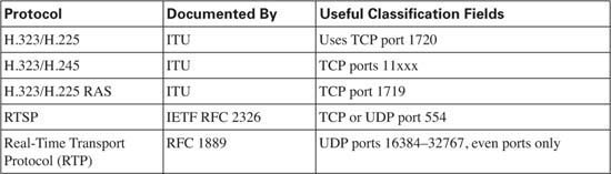
The next few sections of this book examine video more closely in relation to the four QoS characteristics:
![]() Bandwidth
Bandwidth
![]() Delay
Delay
![]() Jitter
Jitter
![]() Loss
Loss
Unlike voice, video uses a variety of packet sizes and packet rates to support a single video stream. Most video codecs take advantage of what can loosely be called “prediction,” by sending an encoded video frame (large packet), followed by a series of vectors describing changes to the previous frame (small packet). Although this type of algorithm greatly reduces the required bandwidth, it does cause video streams to use a dynamic packet rate, with a range of packet sizes. Also the actual average bandwidth required for a section of video depends on the complexity and amount of movement in the video. Table 1-20 lists four popular video codecs and the required bandwidth ranges for each:

Different codecs simply provide different tradeoffs for quality and bandwidth, and many different codecs are needed to support applications of all types. For instance, MPEG includes several standards that were created for different types of applications. ITU H.261 provides a video standard for video conferencing, which works well when the callers do not move around too much! If you have ever been on a video conference and watched someone who used their hands a lot to talk, for instance, you might have seen jerky arm movements. All these codecs operate with dynamic bandwidth, and with different-sized packets. Figure 1-29 shows a packet distribution for percentages of packets at various sizes in an H.261 conference call.

As mentioned earlier, video flows vary both the size of packets sent and the packet rate. In a high-quality video conference that might average 768 kbps of bandwidth, for example, the packet rates might vary from as low as 35 pps to as many as 120 pps. Also, some overhead will be needed for ongoing video signaling traffic. Some QoS tool configuration options might be affected by not only the bandwidth required (kbps), but also by the packet rate (pps). Remember, queue sizes are measured in packets; so to avoid tail drop, a queue holding video traffic may need a much larger queue size than a queue holding voice. Also, Cisco now recommends that when configuring queuing tools for video, you should allow for 20 percent more than the average bandwidth to deal with this small amount of variability in video traffic flows. Cisco also recommends that no more than 33 percent of the link be reserved for video traffic. Table 1-21 summarizes some of the key bandwidth differences between voice and video traffic.

Two-way or interactive packet video experiences the same delay components as does a voice call. However, one-way or streaming packet video tolerates a fairly large amount of delay. Consider Figure 1-30, which shows a packet video device receiving a one-way streaming video stream.

The initial playout delay takes 30 seconds—not 30 ms, but 30 seconds—in the example of Figure 1-30. No interaction occurs, and no video flows back to the video server; by far, the most important feature is that, when the video does play, it has high quality. With a 30-second de- jitter buffer, a cumulative jitter of 30 seconds (not milliseconds) can occur without having playout problems due to delay or jitter.
For two-way interactive packet video, delay of course does impact quality. The previous section about voice and voice delay explains most of what you need to know about video delay. Video experiences codec delay, packetization delay, and de-jitter (initial playout) delay. Of particular note, video delay budgets typically run from 0 to 200 ms for high-quality video conferencing, and de-jitter initial playout delays typically range from 20 to 70 ms.
Just like for delay, one-way video tolerates jitter much more so than two-way, interactive video. When planning for QoS, two-way video should be treated just like voice in terms of minimizing delay. Furthermore, proper and accurate bandwidth allocation/provisioning is recommended. One-way, streaming video should be given enough bandwidth, but extra delay and jitter can be tolerated.
Jitter concerns for video networks can be summarized as follows:
![]() Jitter still happens in packet networks.
Jitter still happens in packet networks.
![]() De-jitter buffers on the receiving side compensate for some jitter.
De-jitter buffers on the receiving side compensate for some jitter.
![]() De-jitter buffers for interactive video typically run in the tens of milliseconds, allowing even small amounts of jitter to affect video quality.
De-jitter buffers for interactive video typically run in the tens of milliseconds, allowing even small amounts of jitter to affect video quality.
![]() De-jitter buffers for streaming video typically run into the tens of seconds, allowing significant jitter to occur without affecting video quality
De-jitter buffers for streaming video typically run into the tens of seconds, allowing significant jitter to occur without affecting video quality
![]() QoS tools, particularly queuing and fragmentation tools, can reduce jitter to low enough values such that the de-jitter buffer for interactive video works effectively.
QoS tools, particularly queuing and fragmentation tools, can reduce jitter to low enough values such that the de-jitter buffer for interactive video works effectively.
Video flows degrade when packets are lost. The picture becomes jerky due to missing frames, the images freeze, and the audio may cut in and out. In short, video does not tolerate loss very well.
Routers drop packets for many reasons; packet loss due to full queues can be addresses with several types of QoS tools. Remember, tail drop describes the situation when a queue fills, another packet needs to be added to the queue, so the router throws away the packet that needs to be added to the tail of the queue. You can use four general QoS strategies to reduce the chance of lost (dropped) video packets:
![]() Enable queuing and putting video in a different queue than bursty data traffic.
Enable queuing and putting video in a different queue than bursty data traffic.
![]() Configure the video queue to be longer.
Configure the video queue to be longer.
![]() Enable CAC to protect the video queue from having too many concurrent video flows in it—in other words, CAC can protect video from other video streams.
Enable CAC to protect the video queue from having too many concurrent video flows in it—in other words, CAC can protect video from other video streams.
![]() Use a Random Early Detect (RED) tool on the loss-tolerant flows (typically data, not video!), which causes those flows to slow down, which in turn reduces overall interface congestion.
Use a Random Early Detect (RED) tool on the loss-tolerant flows (typically data, not video!), which causes those flows to slow down, which in turn reduces overall interface congestion.
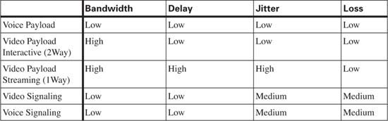
This book, as well as the exams about which this book prepares you, assumes you have a fairly high level of knowledge about data traffic before using this book. In fact, the QoS course assumes that you have been to the ICND and BSCI courses at least, and hopefully the BGP course. In fact, when the Cisco QoS course first came out, the expectation was that students should be CCNPs before attending the course.
QoS has always been important, but QoS has become vitally important with the convergence of data, voice, and video into a single network. As with any convergence of technologies, professionals working in the networking arena come from many different backgrounds. This section about data is intended for those who do not come from a data background.
Note If you want to read more on TCP/IP protocols, take a look at the latest Douglas Comer’s Internetworking with TCP/IP books. Volume 1 is most appropriate for networking engineers. A good alternative is Richard Stevens’s TCP/IP Illustrated, Volume I.
Just like the coverage of voice and video in this chapter, this section breaks down an analysis of data traffic as it relates to the four QoS characteristics: bandwidth, delay, jitter, and loss. The discussion begins with the basics of data application flows, followed by QoS details as they relate to data in terms of the four QoS characteristics.
With voice and video, signaling occurred first in order to create the voice or video call. Although it is not called signaling in the data world, something similar does occur—for instance, when you open a web browser, and browse www.cisco.com, several things happen before the first parts of the web page appear. For our purposes for QoS, this book focuses on the actual payload flows—the actual data—rather than the data equivalent of signaling.
Most applications use one of two TCP/IP transport layer protocols: User Datagram Protocol (UDP) or Transmission Control Protocol (TCP). The person writing the application chooses which transport layer protocol to use. Most of the time the application programmer uses standard protocols, which tell them whether to use TCP or UDP. For instance, web servers use TCP, so if writing a web application, TCP is used.
TCP performs error recovery, but UDP does not. To perform error recovery, TCP sends some initialization messages to create a TCP connection, which coincidentally initializes some counters used to perform the error recovery. Figure 1-31 shows an example of connection establishment.

TCP signals connection establishment using 2 bits inside flags field of the TCP header. Called the SYN and ACK flags, these bits have a particularly interesting meaning. SYN means “synchronize the sequence numbers,” which is one necessary component in initialization for TCP. The ACK field means “the acknowledgment field is valid in this header.”
When the three-way TCP handshake is complete, the TCP connection is up, and error recovery can be performed. Figure 1-32 shows how the sequence and acknowledgment fields are used, after the connection has been established.
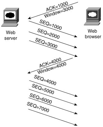
In the figure, the server sends data and labels it with the sequence number. The acknowledgment field in the TCP header sent back to the server by the web client (4,000) implies the next byte to be received; this is called forward acknowledgment. In essence, the browser acknowledged the receipt of all three packets, with sequence numbers 1000, 2000, and 3000. (Each packet contains 1000 bytes of data in this example.) The sequence number reflects the number of the first byte in the segment. Keep in mind that on the packet whose sequence number is 3000, with 1000 bytes, that bytes 3000 to 3999 are in the packet—so the browser should expect to get byte 4000 next.
TCP also controls the rate of sending data using windowing. This window field implies the maximum number of unacknowledged bytes allowed outstanding at any instant in time. Figure 1-34 shows windowing with a current window size of 3000, which increases to a window of 4000 by the end of the example. (Remember, each TCP segment has 1000 bytes of data in this example.) The window then “slides” up and down based on network performance, so it is sometimes called a sliding window. When the sender sends enough bytes to consume the current window, the sender must wait for an acknowledgment, which controls the flow of data. Effectively, the available window decreases as bytes are sent and increases as acknowledgment for those bytes are received.
The biggest difference between TCP and UDP is that TCP performs error recovery. Therefore, some people refer to TCP as reliable, and UDP as unreliable. And remember, voice and video flows that use RTP also use UDP—so why would voice and video use a protocol that is unreliable? The answer is simple: By the time a voice or video packet was sent, and TCP noticed that the packet was lost, and caused a retransmission, far too much delay would have already occurred. Therefore, resending the voice or video packet would be pointless. For data applications, however, where all the data really does need to make it to the other side of the connection, even if it takes additional time, TCP can be very useful. Figure 1-33 outlines the basic error-recovery logic of TCP.

Figure 1-33 depicts a flow where the second TCP segment was lost or was in error. The web client’s reply has an ACK field equal to 2000, implying that the web client is expecting byte number 2000 next. The TCP function at the web server then could recover lost data by resending the second TCP segment. The TCP protocol allows for resending just that segment and then waiting, hoping that the web client will reply with an acknowledgment that equals 4000.
Finally, you should understand one additional feature of TCP and UDP before continuing with your examination of QoS. That feature concerns a part of the TCP and UDP headers called the source and destination port numbers. The main purpose for port numbers can be seen with a simple example; for QoS, port numbers can be used to classify a packet, which in turn allows a router or switch to choose a different QoS action. In this case, Hannah is using three applications, and server Jessie is the server for all three applications. This particular company wrote an Advertising application and a wire-transfer application, both in use. In addition, Hannah is using a web-based application, as shown in Figure 1-34.

After receiving a packet, Jessie needs to know which application to give the data to, but all three packets are from the same Ethernet and IP address. You might think that Jessie could look at whether the packet contains a UDP or a TCP header, but, as you see in the figure, two applications (wire transfer and web) both are using TCP. Well, UDP and TCP designers purposefully included a port number field in the TCP and UDP headers to allow multiplexing. “Multiplexing” is the term generally used to describe the capability to determine which application gets the data for each packet. Each of the applications uses a different port number, so Jessie knows which application to give the data to, as seen in Figure 1-35.
Figure 1-35 Hannah Sending Packets to Jessie, with Three Applications Using Port Numbers to Multiplex

Most well-known applications, such as web, FTP, TFTP, Telnet, SMTP, POP3, and so on, use a well-known port. Using an application would be cumbersome if before you used it you had to call someone to find out what port number it uses. With well-known ports, you can assume that web servers use port 80, for instance. For QoS tools, if you want to classify web traffic, you can just look for packets that use port 80.
Certainly, you could spend a career just learning about, and working with, all the protocols inside the realm of TCP/IP. This brief introduction provides a little background that will help with some of the things you will read about in later sections. Table 1-23 lists the key points to remember about TCP and UDP.

The next few sections of this book examine data more closely in relation to the four QoS characteristics: bandwidth, delay, jitter, and loss.
Unlike voice, which consumes a constant amount of bandwidth, and unlike video, which consumes a range of bandwidth, data bandwidth requirements range wildly. Some applications might literally need less than 1 kbps, whereas others would take literally as much bandwidth as they can get.
The bigger question with data bandwidth revolves around OSI Layer 8—the business layer. For instance, how much bandwidth should web traffic get? Well, in many shops, web traffic consumes 80 percent of the network bandwidth used. However, a better question might be “How much bandwidth does important business web traffic get?” A financial-planning web application ought not to have to compete too hard with my surfing the ESPN.com website to check out the latest scores. A stockbroker might prefer that stock quotes get the lowest latency, for instance, and I would just have to wait a little longer to see the latest sports scores.
The other legitimate question with data application flows concerns whether the application is interactive or not. An interactive application needs less bandwidth typically (not always!) than do the typical noninteractive applications. The traditional comparison between Telnet (very low bandwidth) and FTP (takes as much bandwidth as it can get) implies that interactive implies low bandwidth. Well, many interactive applications today are web based, and if the web pages contain large amounts of graphics, the bandwidth required can also be pretty large.
Bandwidth, delay, jitter, and loss characteristics of data traffic vary based on these factors and others. In fact, one data application’s QoS characteristics might be different at two different companies! Because so many factors must be considered, and because it varies from network to network, no one set of requirements really works.
However, do not despair! You should at least consider one perspective on bandwidth, based on business reasons. Simply put, some applications are business critical, and some are not. At a minimum, a QoS strategy should include identifying the critical applications, and giving these application flows the QoS characteristics they need. The rest of the data traffic can take the crumbs that have fallen off the table—or, in QoS terms, be treated as “best-effort” traffic. Table 1-24 summarizes some of the key bandwidth differences between all three types of traffic.
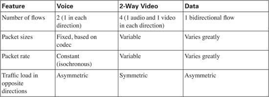
Unlike voice and video, the perceived quality of the data application does not degrade quickly when delay increases by mere hundreds of milliseconds. In fact, relative to voice and interactive video, data applications tolerate delay very well. Also unlike voice and video, data applications tend to have round-trip delay requirements.
Two factors affect the delay requirements of a data application, as summarized in Table 1-25.

Because data QoS requirements vary greatly, more communication happens among the staff when deciding how to treat different applications with QoS. With more communication, the chances of miscommunication increase. If you talk to someone who does not just focus on the network, for instance, he might say “we need consistent 1- to 3-second response time on this mission-critical application!” What he means is that all packets, in both directions, that need to flow, in order for the user to see the complete response from the application, must occur in 1 to 3 seconds. Do not be fooled into thinking that a one-way delay for one packet of 1 to 3 seconds is what the user meant when he asked for 1- to 3-second application response time!
Data applications do not suffer from all the same causes of delay as do voice and video traffic. Earlier in the chapter you learned about the core delay components—queuing, serialization, propagation, network, processing, and shaping. Data does not suffer from the additional delay caused by codec, packetization, and de-jitter buffer delays.
Just like for delay, data application tolerate jitter much more so than voice and video. Interactive applications are much less tolerant of jitter. I learned networking at a large SNA network inside IBM, and the adage when adjusting routes and QoS (built-in to SNA from the early days, but that’s another story!) was that it was okay to have longer response times, as long as the response times were consistent. Human nature for some reason made consistency more important than net response time to most human interactive users, and that fact remains true today.
Interactive data applications cannot tolerate as much jitter or delay as noninteractive applications can. Voice and video applications can tolerate even less jitter or delay than interactive data applications. Because voice and video cannot tolerate any significant delay and jitter, engineers might choose to use QoS tools to decrease jitter for voice and video—which in turn increases delay and jitter for data applications! If a router sends a voice packet next rather than a data packet, for instance, the voice packet has a better chance of meeting its delay budget—but the data packet experiences more delay. Knowing that data can tolerate delay and jitter more than voice enables the engineer to make this tradeoff.
Jitter concerns for data networks can be summarized as follows:
![]() Jitter still happens in packet networks.
Jitter still happens in packet networks.
![]() Data applications do not have a de-jitter buffer—instead, the user always experiences some jitter, perceived simply as variable response times.
Data applications do not have a de-jitter buffer—instead, the user always experiences some jitter, perceived simply as variable response times.
![]() Interactive applications are less tolerant of jitter, but jitter into the hundreds of milliseconds can be tolerated even for interactive traffic.
Interactive applications are less tolerant of jitter, but jitter into the hundreds of milliseconds can be tolerated even for interactive traffic.
![]() In a converged network, QoS tools that improve (lower) jitter are best applied to voice and video traffic; the penalty is longer delays and more jitter for data applications.
In a converged network, QoS tools that improve (lower) jitter are best applied to voice and video traffic; the penalty is longer delays and more jitter for data applications.
Unlike voice and video, data does not always suffer when packets are lost. For most applications, the application needs to get all the data; if the lost packets are re-sent, however, no real damage occurs. Some applications do not even care whether a packet is lost. For perspective, consider applications to fall into one of three categories: those that use UDP and the applications perform error recovery, those that use UDP and the applications do not perform error recovery, and applications that use TCP.
Some applications need error recovery but choose instead to implement the error recovery with application code. For instance, Network File System (NFS) and Trivial File Transfer Protocol (TFTP) both use UDP, and both perform error recovery inside the application. NFS provides the capability to read from and write to remote file servers—certainly guaranteeing that data is not lost would be important to NFS! Likewise, TFTP transfers files, so ensuring that the file was not missing parts would also be important. So, UDP applications that provide application layer recovery tolerate loss.
Some applications simply do not need error recovery. The most popular of these protocols is Simple Network Management Protocol (SNMP), which allows management software to interrogate managed devices for information. Network management stations retrieve huge amounts of individual data, and often times a missed statistic occasionally does not impact the worker using the management software. SNMP designers purposefully avoided TCP and application layer error recovery to keep SNMP simple, and therefore more scalable, knowing that SNMP would be used in large volumes. Because the application does not care whether a packet is lost, these applications tolerate lost packets.
Because TCP-based applications expect TCP to recover lost packets, higher loss rates are acceptable. Although the lost packets may be transparent to the user, the added load on the network caused by retransmission of the packets can actually increase the congestion in the network.

Now you understand bandwidth, delay, jitter, and packet loss, as well as how those things impact voice, video, and data traffic. However, before you can go further with applying these concepts to a real network, you need to step back for a moment and consider a process by which you could examine a network, and then make good choices about how to proceed in implementing QoS.
To that end, the QoS course from Cisco suggests a three-step process for planning and implementing QoS. This is not the only possible process you could use, but it is the one from the QoS course, and the process is directly referenced by one of the exam objectives, so it’s a good one to read through here. While the concepts might be somewhat intuitive, the steps are important. This short section takes a look at that particular process, which runs as follows:

The next few pages examines each step in succession.
When I teach QoS courses, I sometimes jokingly ask if everyone in the room knows all the types of traffic running through their networks. Seldom does anyone confidently say that they really do know what’s running through their network. Do they have a good idea of the main applications, and the protocols they use? Sure. But seldom do people have a real sense for how much bandwidth is being used, or is needed, by a certain set of applications.
Step 1 in this 3-step process suggests that you should identify the traffic, which really boils down to a technical step (Step 1a), and a business step (Step 1b):
Step 1a Perform a network audit by using trace analysis tools, management tools, Network-Based Application Recognition (NBAR), or any other tool to identify protocols and traffic volume
Step 1b Perform a business audit to determine the importance of the discovered traffic types to the business
Step 1b might actually end up being the more difficult of the two because the network audit tends to be a very objective task, whereas the business audit can be a bit subjective.
In Step 1, you need to decide for each type of traffic what “its requirements” are, to quote the actual verbiage. Well, you’ve already read a lot about what different types of traffic need—but that’s not what this step means. Instead, it boils down to service levels. What level of service does each type of traffic need to have in order to meet business goals? That’s a hard question to answer. The concepts you’ve read about in this chapter will certainly be useful in making these choices, but you will also need to look at how much of each type of traffic will go to each site, find out current performance levels, and other analysis before deciding on an appropriate set of service levels for each traffic class.
After completing Step 1, you should have a pretty good idea about the specific different types of traffic in your network. However, there might be lots of different types of traffic. This step suggests that you make decisions about which types of traffic end up in the same traffic class or service class.
The term service class refers to a set of one or more types of traffic that will be treated the same in terms of QoS. For instance, at Step 1 you might have examined five different mission critical applications, and defined service levels for each. However, if all five applications require the same QoS characteristics, then you can place all packets from all five applications into the same service class. You will define service classes in your router and switch configurations so that the router and switch QoS tools can attempt to provide the right levels of bandwidth, delay, jitter, and loss.
So, an expanded definition of this step might be to place each known type of traffic into a service class, with the intent to provide each service class with a unique quality of service.
The number of service classes will vary from site to site. However, for voice and video, you will likely end up with 3 classes:
![]() One for voice payload—The reason that most sites end up with all voice payload in one service class is that the voice calls have the same QoS requirements.
One for voice payload—The reason that most sites end up with all voice payload in one service class is that the voice calls have the same QoS requirements.
![]() One for video payload—Video differs from voice slightly, with variable packet rates, and a slightly variable bit rate, as compared to constant packet and bit rates for a voice call. As a result, it makes sense to separate voice and video into separate service classes
One for video payload—Video differs from voice slightly, with variable packet rates, and a slightly variable bit rate, as compared to constant packet and bit rates for a voice call. As a result, it makes sense to separate voice and video into separate service classes
![]() One for both voice and video signaling traffic—Voice and video signaling traffic is actually more like a data application than voice or video, at least in terms of QoS. The signaling protocols tolerate delay and jitter very well, making them good candidates to be in a separate service class from voice and video.
One for both voice and video signaling traffic—Voice and video signaling traffic is actually more like a data application than voice or video, at least in terms of QoS. The signaling protocols tolerate delay and jitter very well, making them good candidates to be in a separate service class from voice and video.
For data, you might end up with only one or two service classes, or a lot. Cisco tends to highlight the following general classes in the QoS course:
![]() Mission Critical—typically interactive, with significant importance to the business
Mission Critical—typically interactive, with significant importance to the business
![]() Transactional—typically interactive, important to the business
Transactional—typically interactive, important to the business
![]() Best-Effort—General web browsing, e-mail, other unspecified traffic
Best-Effort—General web browsing, e-mail, other unspecified traffic
![]() Scavenger (Less-than-best-effort)—Known types of insignificant or troublesome traffic, for instance, Napster or KaZaa
Scavenger (Less-than-best-effort)—Known types of insignificant or troublesome traffic, for instance, Napster or KaZaa
At the end of this step, you should have a written record of exactly what types of traffic end up in each class. The only exception is the best effort class, which by definition catches all the traffic that was not otherwise specified to be in some other service class.
A QoS policy is a written document that defines the QoS-related service levels for each service class. Essentially, the QoS policy includes the documentation of the work performed in the first two steps, plus the definitions of the QoS actions that should be taken in the routers and switches in order to reach the service levels defined in the QoS policy document.
In order for a QoS policy to actually provide a particular level of service, the policy defines actions to be taken on the packets inside a service class. These actions cause some change in the bandwidth, delay, jitter, and/or loss characteristics of those packets. For instance, a QoS policy might call for a queuing tool to give a guaranteed amount of bandwidth to a class of traffic. Another example might be to more aggressively discard one service class’s packets, in order to reduce packet loss for another service class. A QoS policy might set a limit to the amount of bandwidth allowed for a service class, in order to prevent that service class from taking more bandwidth than it should.
While these steps may seem somewhat intuitive, once you read more about the QoS tools themselves, particular those that use the Modular QoS CLI (MQC), you will see that this 3-step process does provide a good basic framework with which to attack QoS efforts.
The “Foundation Summary” is a collection of tables and figures that provide a convenient review of many key concepts in this chapter. For those of you already comfortable with the topics in this chapter, this summary could help you recall a few details. For those of you who just read this chapter, this review will help solidify some key facts. For any of you doing your final prep before the exam, these tables and figures will be a convenient way to review the day before the exam.
Table 1-27 outlines some of the behaviors seen when no QoS is applied in a network.

As shown in Figure 1-36, with compression, if a ratio of 2:1 is achieved, the 80-kbps flow will only require 40 kbps in order to be sent across the link—effectively doubling the bandwidth capacity of the link.

Figure 1-37 shows a two-queue system where the first queue gets 25 percent of the bandwidth on the link, and the second queue gets 75 percent of the bandwidth.
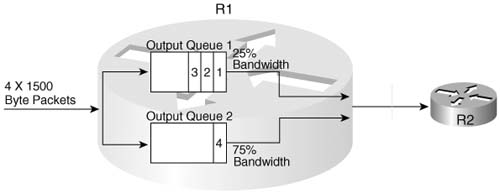
Figure 1-38 shows two contrasting examples of serialization and propagation delay.
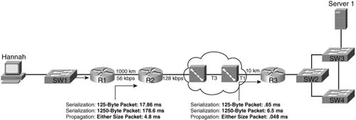
Figure 1-39 lists the queuing, serialization, and propagation delays experienced by data, voice, and video traffic.
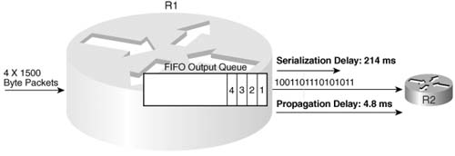
Figure 1-40 depicts LFI operation.
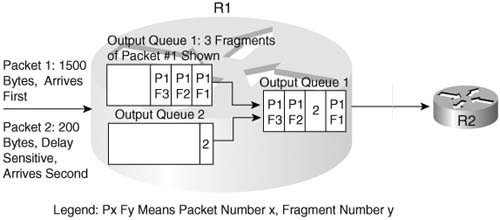
Figure 1-41 shows the jitter experienced by three packets as part of a voice call between phones at extension 301 and 201.
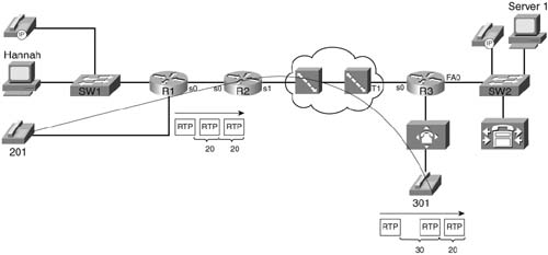
Figure 1-42 outlines the format of an IP packet using RTP.

Table 1-28 lists the bandwidth requirements when using one of two codecs, with varying types of data link protocols.

Figure 1-43 shows an example of delay concepts, with sample delay values shown. When the delay is negligible, the delay is just listed as zero.
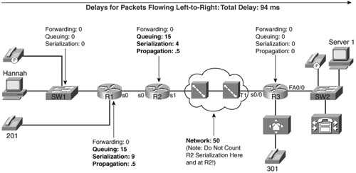
Table 1-29 outlines the suggested delay budgets.

All the delay components for a voice call are summarized in the example in Figure 1-44.

Table 1-30 lists the different delay components and whether they are variable.
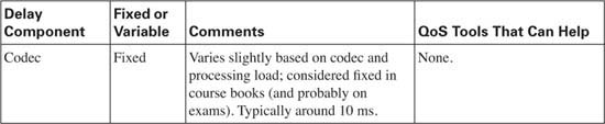
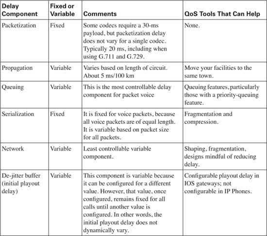
Table 1-31 summarizes the QoS requirements of data, in comparison to voice and video.

As mentioned in the Introduction, you have two choices for review questions. The questions that follow next give you a more difficult challenge than the exam itself by using an open-ended question format. By reviewing now with this more difficult question format, you can exercise your memory better, and prove your conceptual and factual knowledge of this chapter. You can find the answers to these questions in Appendix A.
The second option for practice questions is to use the CD-ROM included with this book. It includes a testing engine and more than 200 multiple-choice questions. You should use this CD-ROM nearer to the end of your preparation, for practice with the actual exam format.
|
1. |
List the four traffic characteristics that QoS tools can affect. |
|
2. |
Describe some of the characteristics of voice traffic when no QoS is applied in a network. |
|
3. |
Describe some of the characteristics of video traffic when no QoS is applied in a network. |
|
4. |
Describe some of the characteristics of data traffic when no QoS is applied in a network. |
|
5. |
Interpret the meaning of the phrase, “QoS is both ‘managed fairness,’ and at the same time ‘managed unfairness’.” |
|
6. |
Define bandwidth. Compare and contrast bandwidth concepts over point-to-point links versus Frame Relay. |
|
7. |
Compare and contrast bandwidth and clock rate in relation to usage for QoS. |
|
8. |
List the QoS tool types that affect bandwidth, and give a brief explanation of why each tool can affect bandwidth. |
|
9. |
Define delay, compare/contrast one-way and round-trip delay, and characterize the types of packets for which one-way delay is important. |
|
10. |
List the categories of delay that could be experienced by all three types of traffic: data, voice, and video. |
|
11. |
Define, compare, and contrast serialization and propagation delay. |
|
12. |
Define network delay. |
|
13. |
List the QoS tool types that affect delay and give a brief explanation of why each tool can affect delay. |
|
14. |
Define jitter. Give an example that shows a packet without jitter, followed by a packet with jitter. |
|
15. |
List the QoS tool types that affect jitter and give a brief explanation of why each tool can affect jitter. |
|
16. |
Define packet loss and describe the primary reason for loss for which QoS tools can help. |
|
17. |
List the QoS tool types that affect loss and give a brief explanation of why each tool can affect loss. |
|
18. |
Describe the contents of an IP packet carrying the payload for a G.729 VoIP call. |
|
19. |
Describe the amount of bandwidth required for G.711 and G.729 VoIP calls, ignoring data-link header/trailer overhead. |
|
20. |
List the delay components that voice calls experience, but which data-only flows do not experience. |
|
21. |
Define the meaning of the term “packetization delay” in relation to a voice call. |
|
22. |
List the different one-way delay budgets as suggested by Cisco and the ITU. |
|
23. |
Define the term “codec delay” and discuss the two components when using a G.729 codec. |
|
24. |
Describe the affects of a single lost packet versus two consecutive lost packets, for a G.729 voice call. |
|
25. |
Describe a typical video payload flow in terms of packet sizes and packet rates. |
|
26. |
Discuss the delay requirements of video traffic. |
|
27. |
List the basic differences between TCP and UDP traffic. |
|
28. |
Contrast the QoS characteristics needed by interactive data applications, as compared to the QoS needs of voice payload flows. |
|
29. |
What are the three steps suggested in this chapter for planning QoS policy implementation? |
|
30. |
The chapter provides a suggested process for planning and implementing QoS policies. The first step involves identifying traffic classes and requirements. That step lists two specific types of audits that should be performed in this step. List and give a brief description of the two audit steps. |
|
31. |
Early in the chapter, a couple of different definitions of QoS were supplied. Paraphrase your own general definition of the term “QoS”. |
|
32. |
What is the purpose of service classes when implementing a QoS policy? |
|
33. |
What are the three steps suggested in this chapter for planning QoS policy implementation? |
|
34. |
The chapter provides a suggested process for planning and implementing QoS policies. The first step involves identifying traffic classes and requirements. That step lists two specific types of audits that should be performed in this step. List and give a brief description of the two audit steps. |
|
35. |
Early in the chapter, a couple of different definitions of QoS were supplied. Paraphrase your own general definition of the term “QoS”. |
|
36. |
What is the purpose of service classes when implementing a QoS policy? |