Chapter 5. Congestion Management
QoS Exam Topics
This chapter covers the following exam topics specific to the QoS exam:
![]() List and explain the different queuing algorithms
List and explain the different queuing algorithms
![]() Explain the components of hardware and software queuing systems on Cisco routers and how they are affected by tuning and congestion
Explain the components of hardware and software queuing systems on Cisco routers and how they are affected by tuning and congestion
![]() Describe the benefits and drawbacks of using WFQ to implement QoS
Describe the benefits and drawbacks of using WFQ to implement QoS
![]() Explain the purpose and features of Class-Based WFQ (CBWFQ)
Explain the purpose and features of Class-Based WFQ (CBWFQ)
![]() Explain the purpose and features of Low Latency Queuing (LLQ)
Explain the purpose and features of Low Latency Queuing (LLQ)
![]() Identify the Cisco IOS commands required to configure and monitor LLQ on a Cisco router
Identify the Cisco IOS commands required to configure and monitor LLQ on a Cisco router
Most people understand the basic concepts of queuing, because most of us experience queuing every day. We wait in line to pay for groceries, we wait for a bank teller, we wait to get into a ride at an amusement park, and so on. So, most of the queuing concepts inside this chapter are intuitive.
Cisco uses the term “congestion management” to refer to queuing systems in their products. This chapter begins with coverage of some queuing concepts inside Cisco routers, including the distinction between hardware and software queues, and where software queues can be used. (Queuing inside LAN switches, particularly the Cisco 2950 series switches, is covered in Chapter 9, “LAN QoS.”)
Following that, the second and third sections of the three major sections in this chapter cover specifics about several Queuing mechanisms available inside Cisco routers. The first of these two sections covers only concepts about several older Queuing tools. The final section covers both concepts and configuration for the three major queuing mechanisms covered by the current QoS exam, namely WFQ, CBWFQ, and LLQ.
The purpose of the “Do I Know This Already?” quiz is to help you decide if you really need to read the entire chapter. If you already intend to read the entire chapter, you do not necessarily need to answer these questions now.
The 12-question quiz, derived from the major sections in “Foundation Topics” portion of the chapter, helps you determine how to spend your limited study time.
Table 5-1 outlines the major topics discussed in this chapter and the “Do I Know This Already?” quiz questions that correspond to those topics.
Caution The goal of self-assessment is to gauge your mastery of the topics in this chapter. If you do not know the answer to a question or are only partially sure of the answer, mark this question wrong for purposes of the self-assessment. Giving yourself credit for an answer you correctly guess skews your self-assessment results and might provide you with a false sense of security.
You can find the answers to the “Do I Know This Already?” quiz in Appendix A, “Answers to the ‘Do I Know This Already?’ Quizzes and Q&A Sections.” The suggested choices for your next step are as follows:
![]() 10 or less overall score—Read the entire chapter. This includes the “Foundation Topics,” the “Foundation Summary,” and the “Q&A” sections.
10 or less overall score—Read the entire chapter. This includes the “Foundation Topics,” the “Foundation Summary,” and the “Q&A” sections.
![]() 11 or 12 overall score—If you want more review on these topics, skip to the “Foundation Summary” section and then go to the “Q&A” section. Otherwise, move to the next chapter.
11 or 12 overall score—If you want more review on these topics, skip to the “Foundation Summary” section and then go to the “Q&A” section. Otherwise, move to the next chapter.
|
1. |
What is the main benefit of the hardware queue on a Cisco router interface? a. Prioritizes latency-sensitive packets so that they are always scheduled next b. Reserves a minimum amount of bandwidth for particular classes of traffic c. Provides a queue so that as soon as the interface is available to send another packet, the packet can be sent, without requiring an interrupt to the router CPU d. Allows configuration of a percentage of the remaining link bandwidth, after allocating bandwidth to the LLQ and the class-default queue |
|
2. |
A set of queues associated with a physical interface, for the purpose of prioritizing packets exiting the interface, are called which of the following? a. Hardware queues b. Software queues d. TX-queues |
|
3. |
Which of the following commands could change the length of a hardware queue? a. hardware queue-length 10 b. tx-queue length 10 c. hardware 10 d. tx-ring-limit 10 |
|
4. |
What is the main benefit of having FIFO queuing enabled on a Cisco router interface? a. Prioritizes latency-sensitive packets so that they are always scheduled next b. Reserves a minimum amount of bandwidth for particular classes of traffic c. Provides a place to hold packets in RAM until space becomes available in the hardware queue for the interface. d. Provides a queue so that as soon as the interface is available to send another packet, the packet can be sent, without requiring an interrupt to the router CPU e. Allows configuration of a percentage of the remaining link bandwidth, after allocating bandwidth to the LLQ and the class-default queue |
|
5. |
What are the main benefits of CQ being enabled on a Cisco router interface? a. Prioritizes latency-sensitive packets so that they are always scheduled next b. Reserves a minimum amount of bandwidth for particular classes of traffic c. Provides a place to hold packets in RAM until space becomes available in the hardware queue for the interface. d. Provides a queue so that as soon as the interface is available to send another packet, the packet can be sent, without requiring an interrupt to the router CPU e. Allows configuration of a percentage of the remaining link bandwidth, after allocating bandwidth to the LLQ and the class-default queue |
|
6. |
What is the main benefit of enabling PQ on a Cisco router interface? a. Prioritizes latency-sensitive packets so that they are always scheduled next b. Reserves a minimum amount of bandwidth for particular classes of traffic c. Provides a place to hold packets in RAM until the interface becomes available for sending the packet d. Provides a queue so that as soon as the interface is available to send another packet, the packet can be sent, without requiring an interrupt to the router CPU e. Allows configuration of a percentage of the remaining link bandwidth, after allocating bandwidth to the LLQ and the class-default queue |
|
7. |
Which of the following are reasons why WFQ might discard a packet instead of putting it into the correct queue? a. The hold-queue limit for all combined WFQ queues has been exceeded. b. The queue length for the flow has passed the WRED minimum drop threshold. c. The WFQ queue length for the queue where the newly-arrived packet should be placed has exceeded the CDT d. ECN feedback has been signaled, requesting that the TCP sender slow down |
|
8. |
Which of the following settings cannot be configured for WFQ on the fair-queue interface subcommand? a. CDT b. Number of queues c. Number of RSVP-reserved queues d. Hold Queue limit e. WRED thresholds |
|
9. |
Examine the following configuration snippet. If a new class, called class3, was added to the policy-map, which of the following commands could be used to reserve 25 kbps of bandwidth for the class? policy-map fred class class1 priority 20 class class2 bandwidth 30 ! interface serial 0/0 bandwidth 100 service-policy output fred a. priority 25 b. bandwidth 25 c. bandwidth percent 25 d. bandwidth remaining-percent 25 |
|
10. |
Examine the following configuration snippet. How much bandwidth does IOS assign to class2? policy-map fred class class1 priority percent 20 class class2 bandwidth remaining percent 20 interface serial 0/0 bandwidth 100 service-policy output fred a. 10 kbps b. 11 kbps c. 20 kbps d. 21 kbps e. Not enough information to tell |
|
11. |
What is the largest number of classes inside a single policy map that can be configured as an LLQ? a. 1 b. 2 c. 3 d. more than 3 |
|
12. |
To prevent non-LLQ queues from being starved, LLQ can police the low-latency queue. Looking at the configuration snippet below, what must be changed or added to cause this policy-map to police traffic in class1? policy-map fred class class1 priority 20 class class2 bandwidth remaining percent 20 interface serial 0/0 bandwidth 100 service-policy output fred a. Change the priority 20 command to priority 20 500, setting the policing burst size b. Add the police 20000 command under class1 c. Nothing – the priority command implies that policing will also be performed d. Add the LLQ-police global configuration command |
Queuing has an impact on all four QoS characteristics directly—bandwidth, delay, jitter, and packet loss. Many people, upon hearing the term “QoS,” immediately think of queuing, but QoS includes many more concepts and features than just queuing. Queuing is certainly the most often deployed and most important QoS tool.
This chapter begins by explaining the core concepts about queuing. Following that, most queuing tools are covered, including additional concepts specific to that tool, configuration, monitoring, and troubleshooting.
Most people already understand many of the concepts behind queuing. First, this section explains the basics and defines a few terms. Afterward, some of the IOS-specific details are covered.
IOS stores packets in memory while processing the packet. When a router has completed all the required work except actually sending the packet, if the outgoing interface is currently busy, the router just keeps the packet in memory waiting on the interface to become available. To manage the set of packets sitting around in memory waiting to exit an interface, IOS creates a queue. A queue just organizes the packets waiting to exit an interface; the queue itself is nothing more than a series of pointers to the memory buffers that hold the individual packets that are waiting to exit the interface.
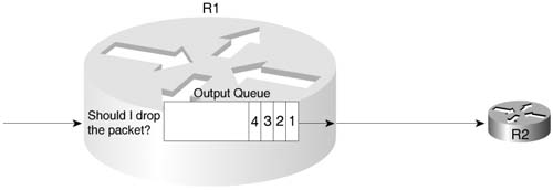
The most basic queuing scheme uses a single queue, with first-in, first-out (FIFO) scheduling. What does that mean? Well, when the IOS decides to take the next packet from the queue, of those packets still in the queue, it takes the one that arrived earlier than all the other packets in the queue. Figure 5-1 shows a router, with an interface using a single FIFO queue.

Although a single FIFO queue seems to provide no QoS features at all, it actually does affect drop, delay, and jitter. Because there is only one queue, the router need not classify traffic to place it into different queues. Because there is only one queue, the router need not worry about how to decide from which queue it should take the next packet — there is only one choice. And because this single queue uses FIFO logic, the router need not reorder the packets inside the queue.
However, the size of the output queue affects delay, jitter, and loss. Because the queue has a finite size, it may fill. If it fills, and another packet needs to be added to the queue, tail drop would cause the packet to be dropped. One solution to the drops would be to lengthen the queue, which decreases the likelihood of tail drop. With a longer queue, however, the average delay increases, because packets may be enqueued behind a larger number of other packets. In most cases when the average delay increases, the average jitter increases as well. The following list summarizes the key concepts regarding queue length:
![]() With a longer queue length, the chance of tail drop decreases as compared with a shorter queue, but the average delay increases, with the average jitter typically increasing as well.
With a longer queue length, the chance of tail drop decreases as compared with a shorter queue, but the average delay increases, with the average jitter typically increasing as well.
![]() With a shorter queue length, the chance of tail drop increases as compared with a longer queue, but the average delay decreases, with the average jitter typically decreasing as well.
With a shorter queue length, the chance of tail drop increases as compared with a longer queue, but the average delay decreases, with the average jitter typically decreasing as well.
![]() If the congestion is sustained such that the offered load of bytes trying to exit an interface exceeds the interface speed for long periods, drops will be just as likely whether the queue is short or long.
If the congestion is sustained such that the offered load of bytes trying to exit an interface exceeds the interface speed for long periods, drops will be just as likely whether the queue is short or long.
To appreciate most queuing concepts, you need to consider a queuing system with at least two queues. Consider Figure 5-2, which illustrates two FIFO output queues.

Figure 5-2 illustrates the questions that are answered by the queuing tool. Step 1, the classification step, works like classification and marking tools, except the resulting action is to place a packet in a queue, as opposed to marking a packet. So, at Step 1, the packet header is examined, and depending on the matched values, the packet is placed into the appropriate queue. Before placing the packet in the queue, the router must make sure that space is available, as shown in Step 2 in Figure 5-2. If no space is available, the packet is dropped. Inside each queue, the packets can be reordered (step 3): in this example, however, each queue uses FIFO logic inside each queue, so the packets would never be reordered inside the queue. Finally, the queuing system must choose to take the next packet for transmission from either Queue 1 or Queue 2 (Step 4). The scheduler makes the decision at Step 4.
Although the classification portion of each queuing tool is relatively obvious, consider two related points when thinking about classification by a queuing tool. First, with a QoS strategy that causes classification and marking to occur near the ingress edge of the network, the queuing tool may enqueue packets that have already been marked. So, the queuing tool can classify based on these marked fields, which was the whole point in marking them in the first place! Second, for each category of traffic for which you want to provide different queuing treatment, you need a different queue. For instance, you may want to classify traffic into six classes for queuing, so each class can get different treatment in a different queue. If the queuing tool only supports four different queues, you may need to consider a different queuing tool to support your QoS policy.
Inside each queue, the queuing methods use FIFO Queuing. The interesting logic for queuing occurs after the packets have been enqueued, when the router decides from which queue to take the next packet. Queue scheduling describes the process of the device, in this case a router, choosing which queue to service next. This process is also called a service algorithm, or a queue service algorithm. The scheduler may reserve amounts of bandwidth, or a percentage of link bandwidth, for a particular queue. The scheduler may always service one queue first, which means the packets in that queue will experience very low delay and jitter.
For the exams, you need to know what each queuing tool’s scheduler accomplishes; for some tools, however, you also need to know the internals of how the scheduler actually works.
Note Cisco leads the industry in making details about their products public (being the first large networking vendor to publish bug reports, for instance). However, Cisco must also protect their intellectual assets. So, for some of the newer queuing tools, Cisco has not yet published every detail about how the scheduling algorithm works. For some of the older queuing tools, the details are published. Frankly, the details of how the scheduling code works inside IOS might be interesting, but it is not really necessary for a deep understanding of what a queuing tool does. For the QoS exams, you need to know what each queuing tool’s scheduler accomplishes; for some tools, however, you also need to know the internals of how the scheduler actually works. When necessary, this book gives you plenty of details about the internal scheduling algorithms to help prepare you for the exams.
A final comment about the core concepts of queuing: The size of each packet does not affect the length of the queue, or how many packets it can hold. A queue of length 10 holds ten 1500-byte packets as easily as it holds ten 64-byte packets. Queues actually do not hold the packets themselves, but instead just hold pointers to the packets, whose contents are held in buffers.
Table 5-2 summarizes the key concepts of queuing. This table is used to compare the various queuing tools in the “Queuing Tools” section of this chapter.

The queues described so far in this chapter are created by the software in a router, namely Cisco IOS. However, when a queuing scheduler decides which packet to send next, the packet does not move directly out the interface. Instead, the router moves the packet from the interface software queue to another small FIFO queue on each interface. Cisco calls this separate, final queue either the Transmit Queue (TX Queue) or Transmit Ring (TX Ring), depending on the model of the router. Regardless of which name is used, for the purposes of this book and the QoS exam, you can call this small FIFO queue a Hardware Queue, TX Queue, or TX Ring. Throughout this book, you can consider all three names for the hardware queue to be equivalent.
The Hardware Queue’s objective is to drive the link utilization to 100 percent when packets are waiting to exit an interface. The Hardware Queue holds outgoing packets so that the interface does not have to rely on the general-purpose processor in the router in order to start sending the next packet. The Hardware Queue can be accessed directly by the application-specific integrated circuits (ASICs) associated with an interface, so even if the general processor is busy, the interface can begin sending the next packet without waiting for the router CPU. Because the most constrained resource in a router is typically the bandwidth on the attached interfaces, particularly on WAN interfaces, the router hopes to always be able to send the next packet immediately when the interface finishes sending the last packet. The Hardware Queue provides a key component to reach that goal.
However, the existence of the Hardware Queue does impact queuing to some extent. Figure 5-3 depicts the Hardware Queue, along with a single FIFO software queue.

Two different examples are outlined in Figure 5-3. In the top part of the figure, the scenario begins with no packets in the software queue, and no packets in the Hardware Queue. Then, four packets arrive. With a Hardware Queue with room for four packets, all four packets are placed into the Hardware Queue.
In the second example, any new packets that arrive will be placed into the software queue. Assuming that the software queue and the Hardware Queue were empty before the seven packets shown in the figure arrived, the first four packets would have been placed in the Hardware queue, and the last three in the software queue. So, any new packets will be placed at the end of the software queue.
All the queuing tools in IOS create and manage interface Software queues, not interface Hardware Queues. Each interface uses one TX Queue (or TX Ring), and the Hardware Queue is a FIFO queue, unaffected by the queuing configuration on the interface.
In Figure 5-3, the packets are sent in the same order that they would have been sent if the Hardware Queue did not exist. In some cases, however, the Hardware Queue impacts the results of the software queuing scheduler. For instance, consider Figure 5-4, where queuing is configured with two software queues. In this scenario, six packets arrive, numbered in the order in which they arrive. The software queuing configuration specifies that the first two packets (1 and 2) should be placed into Queue 2, and the next four packets (numbered 3 through 6) should be placed into Queue 1.

Many people assume that the router behaves as shown in the top part of Figure 5-4, with the scheduler determining the order in which packets exit the interface. In reality, IOS behaves as shown in the bottom half of Figure 5-4. In the top half of the figure, if all six packets were to arrive instantaneously, all six packets would be placed into the appropriate software queue. If this particular queuing tool’s scheduler always serviced packets from Queue 1, and only serviced Queue 2 if Queue 1 was empty, the packets will leave in a different order than they arrived. In fact, packets 3 through 6 would exit in order, and then packets 1 and 2 would be sent. Ultimately, the order would just depend on the logic of the scheduling part of the queuing tool.
In this particular example, however, the packets would actually exit the interface in the same order that the packets were received because of the existence of the Hardware Queue. As mentioned earlier, when the router identifies the output interface for a packet, it checks the Hardware Queue for that interface. If space is available, the packet is placed in the Hardware Queue, and no output queuing is performed for that packet. In the example, because the scenario assumes that no other packets were waiting to exit R1’s S0/0 interface before these six packets arrive, the first two packets are placed in the Hardware Queue. When packet 3 arrives, S0/0’s Hardware Queue is full, so packets 3 through 6 are placed into an interface software queue, based on the queuing configuration for R1’s S0/0 interface. The queuing classification logic places packets 3 through 6 into Queue 1. The router drains the packets in order from the TX Queue, and moves packets 3, 4, 5, and 6, in order, from Queue 1 into the Hardware Queue. The actual order that the packets exit S0 is the same order as they arrived.
IOS automatically attempts to minimize the impact of the Hardware Queue to the IOS queuing tools. The IOS maintains the original goal of always having a packet in the Hardware Queue, available for the interface to immediately send when the interface completes sending the previous packet. When any form of software queuing tool is enabled on an interface, IOS on lower-end routers typically reduces the size of the Hardware Queue to a small value, often times to a length of 2. The smaller the value, the less impact the TX Queue has on the effects of the queuing method.
In some cases, you may want to change the setting for the size of the Hardware Queue. For instance, the QoS course makes a general recommendation of size 3 for slow speed serial interfaces, although I personally believe that size 2 works well, and is the default setting on many router platforms once queuing has been configured. Also, ATM interfaces typically require a little thought for Hardware Queue lengths, as described at http://www.cisco.com/en/US/tech/tk39/tk824/technologies_tech_note09186a00800fbafc.shtml. (If you can’t find the URL, go to www.cisco.com, and search on “Understanding and Tuning the tx-ring-limit Value.”) Example 5-1 lists several commands that enable you to examine the size of the Hardware Queue, and change the size. (Keep in mind the other names for the Hardware Queue—TX Ring and TX Queue.)
Example 5-1 TX Queue Length: Finding the Length, and Changing the Length
Interface Serial0/0
Hardware is PowerQUICC MPC860
DCE V.35, clock rate 1300000
idb at 0x8108F318, driver data structure at 0x81096D8C
SCC Registers:
General [GSMR]=0x2:0x00000030, Protocol-specific [PSMR]=0x8
Events [SCCE]=0x0000, Mask [SCCM]=0x001F, Status [SCCS]=0x06
Transmit on Demand [TODR]=0x0, Data Sync [DSR]=0x7E7E
Interrupt Registers:
Config [CICR]=0x00367F80, Pending [CIPR]=0x00008000
Mask [CIMR]=0x40204000, In-srv [CISR]=0x00000000
Command register [CR]=0x600
Port A [PADIR]=0x1100, [PAPAR]=0xFFFF
[PAODR]=0x0000, [PADAT]=0xEFFF
Port B [PBDIR]=0x09C0F, [PBPAR]=0x0800E
[PBODR]=0x0000E, [PBDAT]=0x3E77D
Port C [PCDIR]=0x00C, [PCPAR]=0x000
[PCSO]=0xC20, [PCDAT]=0xFC0, [PCINT]=0x00F
Receive Ring
rmd(68012830): status 9000 length 1F address 3D3FC84
rmd(68012838): status 9000 length 42 address 3D41D04
rmd(68012840): status 9000 length F address 3D43D84
rmd(68012848): status 9000 length 42 address 3D43084
rmd(68012850): status 9000 length 42 address 3D3E904
rmd(68012858): status 9000 length 157 address 3D43704
Transmit Ring
tmd(680128B0): status 5C00 length 40 address 3C01114
tmd(680128B8): status 5C00 length D address 3C00FD4
tmd(680128C0): status 5C00 length 40 address 3C00FD4
tmd(680128C8): status 5C00 length D address 3C00E94
tmd(680128D0): status 5C00 length 11A address 3D6E394
tmd(680128D8): status 5C00 length 40 address 3C019D4
tmd(680128E0): status 5C00 length 40 address 3C01ED4
tmd(680128E8): status 5C00 length D address 3D58BD4
tmd(680128F0): status 5C00 length 40 address 3D58954
tmd(680128F8): status 5C00 length 40 address 3D59214
tmd(68012900): status 5C00 length D address 3D59494
tmd(68012910): status 5C00 length 40 address 3C00214
tmd(68012918): status 5C00 length D address 3C01C54
tmd(68012920): status 5C00 length 40 address 3C005D4
tmd(68012928): status 7C00 length 40 address 3C00714
SCC GENERAL PARAMETER RAM (at 0x68013C00)
Rx BD Base [RBASE]=0x2830, Fn Code [RFCR]=0x18
Tx BD Base [TBASE]=0x28B0, Fn Code [TFCR]=0x18
Max Rx Buff Len [MRBLR]=1548
Rx State [RSTATE]=0x18008440, BD Ptr [RBPTR]=0x2840
Tx State [TSTATE]=0x18000548, BD Ptr [TBPTR]=0x28C8
SCC HDLC PARAMETER RAM (at 0x68013C38)
CRC Preset [C_PRES]=0xFFFF, Mask [C_MASK]=0xF0B8
Errors: CRC [CRCEC]=0, Aborts [ABTSC]=0, Discards [DISFC]=0
Nonmatch Addr Cntr [NMARC]=0
Retry Count [RETRC]=0
Max Frame Length [MFLR]=1608
Rx Int Threshold [RFTHR]=0, Frame Cnt [RFCNT]=65454
User-defined Address 0000/0000/0000/0000
User-defined Address Mask 0x0000
buffer size 1524
PowerQUICC SCC specific errors:
0 input aborts on receiving flag sequence
0 throttles, 0 enables
0 overruns
0 transmitter underruns
0 transmitter CTS losts
0 aborted short frames
!!!!!!!!!!!!!!!!!!!!!!!!!!!!!!!!!!!!!!!!!!!!!!!!!!!!!!!!!!!!!!!!!
R3#conf t
Enter configuration commands, one per line. End with CNTL/Z.
R3(config)#int s 0/0
!!!!!!!!!!!!!!!!!!!!!!!!!!!!!!!!!!!!!!!!!!!!!!!!!!!!!!!!!!!!!!!!!!
R3#show controllers serial 0/0
01:03:09: %SYS-5-CONFIG_I: Configured from console by console
Interface Serial0/0
!!!!! Lines omitted to save space
R3#conf t
Enter configuration commands, one per line. End with CNTL/Z.
R3(config)#int s 0/0
R3(config-if)#no priority-group 1
R3(config-if)#tx-ring-limit 1
R3(config-if)#^Z
!!!!!!!!!!!!!!!!!!!!!!!!!!!!!!!!!!!!!!!!!!!!!!!!!!!!!!!!!!!!!!!!!!
R3#show controllers serial 0/0
Interface Serial0/0
! Lines omitted to save space
! Lines omitted to save space
The show controllers serial 0/0 command lists the size of the TX Queue or TX Ring. In the shaded output in Example 5-1, the phrase “tx_limited=0(16)” means that the TX Ring (Hardware Queue) holds 16 packets. The zero means that the queue size is not currently limited due to a queuing tool being enabled on the interface. For the first instance of show controllers, no queuing method is enabled on the interface, so a zero signifies that the size of the TX Ring has not been limited automatically.
After enabling Priority Queuing with the priority-group interface subcommand, the next show controllers command lists “tx_limited=1(2).” The new length of the TX Ring is 2, and 1 means that the length is automatically limited as a result of queuing being configured. Next, Priority Queuing is disabled with the no priority-group interface subcommand, but the length of the TX Ring is explicitly defined with the tx-ring-limit 1 interface subcommand. On the final show controllers command, the “tx_limited=0(1)” output implies that the size is not limited, because no queuing is enabled, but that the length of the TX Ring is 1.
The following list summarizes the key points about Hardware Queues in relation to their effect on software queuing:
![]() The Hardware Queue always performs FIFO scheduling, and cannot be changed.
The Hardware Queue always performs FIFO scheduling, and cannot be changed.
![]() The Hardware Queue uses a single queue, per interface.
The Hardware Queue uses a single queue, per interface.
![]() IOS shortens the interface Hardware Queue automatically when an software queuing method is configured.
IOS shortens the interface Hardware Queue automatically when an software queuing method is configured.
![]() The Hardware Queue length can be configured to a different value.
The Hardware Queue length can be configured to a different value.
IOS queuing tools create and manage Software Queues associated with an interface, and then the packets drain into the Hardware Queue associated with the interface. IOS also supports queuing on Frame Relay subinterfaces and individual Frame Relay VCs when traffic shaping is also enabled, as well as for individual ATM VCs. Shaping queues, created by the traffic-shaping feature, drain into the interface output queues, which then drain into the Hardware Queue. Like the interface Software Queues, the shaping queues and ATM per-VC queues can be managed with IOS queuing tools. (In this book, the specific coverage shows queuing tools applied to the queues created by Shaping tools for Frame Relay.)
The interaction between shaping queues associated with a subinterface or VC, and software queues associated with a physical interface, is not obvious at first glance. So, before moving into the details of the various queuing tools, consider what happens on subinterfaces, VCs, and physical interfaces so that you can make good choices about how to enable queuing in a router.
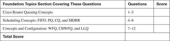
Figure 5-5 provides a reasonable backdrop from which to explain the interaction between queues. R1 has many Frame Relay permanent virtual circuits (PVCs) exiting its S0/0 physical interface. The figure shows queues associated with two of the PVCs, a single software queue for the physical interface, and the Hardware Queue for the interface.
In this particular example, each subinterface uses a single FIFO shaping queue; a single software queue is associated with the physical interface. At first glance, it seems simple enough: a packet arrives, and the forwarding decision dictates that the packet should exit subinterface S0/0.1. It is placed into the subinterface 0/0.1 shaping queue, and then into the physical interface software queue, and then into the Hardware Queue. Then, it exits the interface.
In some cases, the packet moves from the shaping queues directly to the Hardware Queue. You may recall that packets are not even placed in the software queue if the Hardware Ring is not full! If no congestion occurs on the interface, the Hardware Ring does not fill. If no congestion occurs in the Hardware Ring, the interface software queue does not fill, and the queuing tool enabled on the interface has no effect on the packets exiting the interface.
In some cases, IOS does not place the packets into a shaping queue as they arrive, but instead the packets are placed into the Software queue or TX Queue. When the shaping features knows that a newly arrived packet does not exceed the shaping rate, there is no need to delay the packet. In that case, a queuing tool used for managing the shaping queue would also have no effect on that particular packet.
Traffic shaping can cause subinterface shaping queues to fill, even when there is no congestion on the physical interface. Traffic shaping, enabled on a subinterface or VC, slows down the flow of traffic leaving the subinterface or VC. In effect, traffic shaping on the subinterface creates congestion between the shaping queues and the physical interface software queues. On a physical interface, packets can only leave the interface at the physical clock rate used by the interface; similarly, packets can only leave a shaping queue at the traffic-shaping rate.
For example, the VC associated with subinterface S0/0.1 uses a 64 kbps committed information rate (CIR), and S0/0 uses a T/1 circuit. Without traffic shaping, more than 64 kbps of traffic could be sent for that PVC, and the only constraining factor would be the access rate (T/1). The Frame Relay network might discard some of the traffic, because the router may send more (up to 1.5 Mbps) on the VC, exceeding the traffic contract (64-kbps CIR). So, traffic shaping could be enabled on the subinterface or VC, restricting the overall rate for this PVC to 64 kbps, to avoid frame loss inside the Frame Relay network. If the offered load of traffic on the subinterface exceeds 64 kbps for some period, traffic shaping delays sending the excess traffic by placing the packets into the shaping queue associated with the subinterface, and draining the traffic from the shaping queue at the shaped rate.
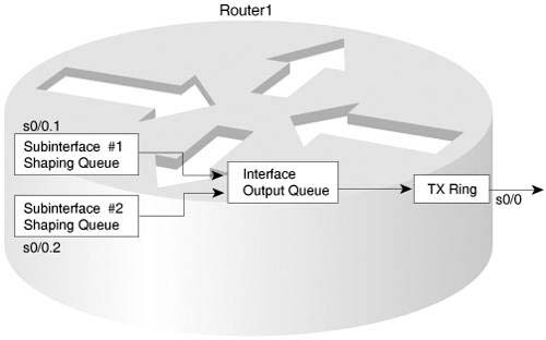
Figure 5-6 shows an updated version of Figure 5-5; this one’s PVC is currently exceeding the shaping rate, and the other PVC is not exceeding the shaping rate. In Figure 5-6, packets arrive and are routed out of each of the two subinterfaces. Traffic for subinterface 0/0.1 exceeds the shaping rate, and packets for subinterface 0/0.2 do not. Therefore, IOS places some packets into the shaping queue for subinterface 0/0.1, because traffic shaping delays packets by queuing the packets. On subinterface 0/0.2, IOS does not queue the packets, because the shaping rate has not been exceeded.
You can configure queuing tools to create and manage the software queues on a physical interface, as well as the shaping queues created by traffic shaping. The concepts in this chapter apply to using software queuing on both the main interface, and on any shaping queues. However, this chapter only covers the configuration of queuing to manipulate the interface software queues. Chapter 6, “Traffic Policing and Shaping,” which covers traffic shaping, explains how to configure queuing for use on shaping queues. When reading the next chapter, keep these queuing concepts in mind and watch for the details of how to enable your favorite queuing tools for shaping queues.
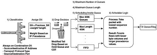
For the remainder of this chapter, queuing tools are compared based on the six general points listed in this section. Figure 5-7 outlines these points in the same sequence that each point is listed in the upcoming sections on each queuing tool.

Scheduling gets the most attention when network engineers choose which queuing tool to use for a particular application. However, the other components of queuing are important as well. For instance, if the classification part of a queuing tool cannot classify the traffic as defined in the QoS policy for the network, either the policy must be changed or another tool must be used. One such example would be that PQ and CQ cannot take direct advantage of network-based application recognition (NBAR), but CBWFQ and LLQ can. In addition, some queuing tools allow a drop policy for each queue, which becomes particularly important when voice and video compete with data traffic in a converged network.
For the purposes of QOS exam preparation, you need to know how Cisco IOS Queuing tools perform scheduling. Scheduling refers to the logic a queuing tool uses to pick the queue from which it will take the next packet. For some Queuing tools, you need to understand only the basic concepts, focusing on the scheduling logic. Those tools and concepts are covered in this section.
Later, in the last and most detailed section of this chapter, you will read about three of the most popular Queuing tools—WFQ, CBWFQ, and LLQ. For these tools, you need to know both the concepts and how to configure the tools.
The first reason that a router needs software queues is to hold a packet while waiting for the interface to become available for sending the packet. Whereas the other queuing tools in this chapter also perform other functions, like reordering packets through scheduling, FIFO Queuing just provides a means to hold packets while they are waiting to exit an interface.
FIFO Queuing does not need the two most interesting features of the other queuing tools, namely classification and scheduling. FIFO Queuing uses a single software queue for the interface. Because there is only one queue, there is no need for classification to decide the queue into which the packet should be placed. Also there is no need for scheduling logic to pick which queue from which to take the next packet. The only really interesting part of FIFO Queuing is the queue length, which is configurable, and how the queue length affects delay and loss.
FIFO Queuing uses tail drop to decide when to drop or enqueue packets. If you configure a longer FIFO queue, more packets can be in the queue, which means that the queue will be less likely to fill. If the queue is less likely to fill, fewer packets will be dropped. However, with a longer queue, packets may experience more delay and jitter. With a shorter queue, less delay occurs, but the single FIFO queue fills more quickly, which in turn causes more tail drops of new packets. These facts are true for any queuing method, including FIFO.
Figure 5-8 outlines simple FIFO Queuing. R1 uses FIFO Queuing on the interface connected to R2. The only decision required when configuring FIFO Queuing is whether to change the length of the queue.
Remember to consider two steps when configuring FIFO Queuing. First, configuring FIFO Queuing actually requires you to turn off all other types of queuing, as opposed to just configuring FIFO Queuing. Cisco IOS uses WFQ as the default queuing method on serial interfaces running at E1 speeds and slower. However, IOS does not supply a command to enable FIFO Queuing; to enable FIFO Queuing, you must first disable WFQ by using the no fair-queue interface subcommand. If other queuing tools have been explicitly configured, you should also disable these. Just by removing all other queuing configuration from an interface, you have enabled FIFO!
The second FIFO configuration step that you might consider is to override the default queue length. To do so, use the hold-queue x out interface subcommand to reset the length of the queue.
Example 5-2 shows a sample FIFO Queuing configuration.
Example 5-2 FIFO Queuing Configuration
Enter configuration commands, one per line. End with CNTL/Z.
R3(config)#int s 0/0
R3(config-if)#no fair-queue
R3(config-if)#^Z
R3#sh int s 0/0
Serial0/0 is up, line protocol is up
Hardware is PowerQUICC Serial
Description: connected to FRS port S0. Single PVC to R1.
MTU 1500 bytes, BW 1544 Kbit, DLY 20000 usec,
reliability 255/255, txload 1/255, rxload 1/255
Encapsulation FRAME-RELAY, loopback not set
Keepalive set (10 sec)
LMI enq sent 80, LMI stat recvd 73, LMI upd recvd 0, DTE LMI up
LMI DLCI 1023 LMI type is CISCO frame relay DTE
Broadcast queue 0/64, broadcasts sent/dropped 171/2, interface broadcasts 155
Last input 00:00:02, output 00:00:03, output hang never
Last clearing of "show interface" counters 00:13:48
Input queue: 0/75/0/0 (size/max/drops/flushes); Total output drops: 0
Output queue :0/40 (size/max)
30 second output rate 0 bits/sec, 0 packets/sec
235 packets input, 14654 bytes, 0 no buffer
Received 0 broadcasts, 0 runts, 0 giants, 0 throttles
2 input errors, 0 CRC, 2 frame, 0 overrun, 0 ignored, 0 abort
264 packets output, 15881 bytes, 0 underruns
0 output errors, 0 collisions, 6 interface resets
0 output buffer failures, 0 output buffers swapped out
10 carrier transitions
DCD=up DSR=up DTR=up RTS=up CTS=up
R3#conf t
Enter configuration commands, one per line. End with CNTL/Z.
R3(config)#int s 0/0
R3(config-if)#hold-queue 50 out
R3(config-if)#^Z
!
R3#sh int s 0/0
Serial0/0 is up, line protocol is up
Hardware is PowerQUICC Serial
! Lines omitted for brevity
Output queue :0/50 (size/max)
Example 5-2 shows FIFO Queuing being configured by removing the default WFQ configuration with the no fair-queue command. The show interface command lists the fact that FIFO Queuing is used, and the output queue has 40 entries maximum. After configuring the output queue to hold 50 packets with the hold-queue 50 out command, the show interface output still lists FIFO Queuing, but now with a maximum queue size of 50.
FIFO Queuing is pretty basic, but it does provide a useful function: It provides the basic queuing function of holding packets until the interface is no longer busy.
Priority Queuing’s most distinctive feature is its scheduler. PQ schedules traffic such that the higher-priority queues always get serviced, with the side effect of starving the lower-priority queues. With a maximum of four queues, called High, Medium, Normal, and Low, the complete logic of the scheduler can be easily represented, as is shown in Figure 5-9.

As seen in Figure 5-9, if the High queue always has a packet waiting, the scheduler will always take the packets in the High queue. If the High queue does not have a packet waiting, but the Medium queue does, one packet is taken from the Medium queue—and then the process always starts over at the High queue. The Low queue only gets serviced if the High, Medium, and Normal queues do not have any packets waiting.
The PQ scheduler has some obvious benefits and drawbacks. Packets in the High queue can claim 100 percent of the link bandwidth, with minimal delay, and minimal jitter. The lower queues suffer, however. In fact, when congested, packets in the lower queues take significantly longer to be serviced than under lighter loads. When the link is congested, user applications may stop working if their packets are placed into lower-priority queues.
The fact that PQ starves lower priority queues makes it a relatively unpopular choice for queuing today. Also, LLQ tends to be a better choice, because LLQ’s scheduler has the capability to service high priority packets first while preventing the higher priority queues from starving the lower priority queues. If you would like to read more about the concepts behind PQ, as well as how to configure it, refer to Appendix B, “Additional QoS Reference Materials,” (found on the book’s accompanying CD-ROM).
Historically, Custom Queuing (CQ) followed PQ as the next IOS queuing tool added to IOS. CQ addresses the biggest drawback of PQ by providing a queuing tool that does service all queues, even during times of congestion. It has 16 queues available, implying 16 classification categories, which is plenty for most applications. The negative part of CQ, as compared to PQ, is that CQ’s scheduler does not have an option to always service one queue first — like PQ’s High queue — so CQ does not provide great service for delay- and jitter-sensitive traffic.
As with most queuing tools, the most interesting part of the tool is the scheduler. The CQ scheduler reserves an approximate percentage of overall link bandwidth to each queue. CQ approximates the bandwidth percentages, as opposed to meeting an exact percentage, due to the simple operation of the CQ scheduler. Figure 5-10 depicts the CQ scheduler logic.
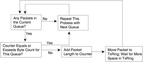
The CQ scheduler performs round-robin service on each queue, beginning with Queue 1. CQ takes packets from the queue, until the total byte count specified for the queue has been met or exceeded. After the queue has been serviced for that many bytes, or the queue does not have any more packets, CQ moves on to the next queue, and repeats the process.
CQ does not configure the exact link bandwidth percentage, but rather it configures the number of bytes taken from each queue during each round-robin pass through the queues. Suppose, for example, that an engineer configures CQ to use five queues. The engineer assigns a byte count of 10,000 bytes for each queue. With this configuration, the engineer has reserved 20 percent of the link bandwidth for each queue. (If each queue sends 10,000 bytes, a total of 50,000 bytes are sent per cycle, so each queue sends 10,000/50,000 of the bytes out of the interface, or 20 percent.) If instead the engineer has assigned byte counts of 5,000 bytes for the first 2 queues, 10,000 for the next 2 queues, and 20,000 for the fifth queue, the total bytes sent in each pass through the queues would again total 50,000 bytes. Therefore, Queues 1 and 2 would get 5,000/50,000, or 10 percent of the link bandwidth. Queues 3 and 4 would get 10000/50000, or 20 percent of the bandwidth, and Queue 5 would get 20000/50000, or 40 percent. The following formula calculates the implied bandwidth percentage for Queue x:
(Byte Count for Queue x)/Sum of Byte Counts for All Queues
The CQ scheduler essentially guarantees the minimum bandwidth for each queue, while allowing queues to have more bandwidth under the right conditions. Imagine that 5 queues have been configured with the byte counts of 5,000, 5,000, 10,000, 10,000, and 20,000 for queues 1 through 5, respectively. If all 5 queues have plenty of packets to send, the percentage bandwidth given to each queue is 10 percent, 10 percent, 20 percent, 20 percent, and 40 percent, as described earlier. However, suppose that Queue 4 has no traffic over some short period of time. For that period, when the CQ scheduler tries to service Queue 4, it notices that no packets are waiting. The CQ scheduler moves immediately to the next queue. Over this short period of time, only Queues 1 through 3 and Queue 5 have packets waiting. In this case, the queues would receive 12.5 percent, 12.5 percent, 25 percent, 0 percent, and 50 percent of link bandwidth, respectively. (The math to get these percentages is number-of-bytes-per-cycle/40,000 because around 40,000 bytes should be taken from the four active queues per cycle.) Note also that queues that have not been configured are automatically skipped.
Unlike PQ, CQ does not name the queues, but it numbers the queues 1 through 16. No single queue has a better treatment by the scheduler than another, other than the number of bytes serviced for each queue. So, in the example in the last several paragraphs, Queue 5, with 20000 bytes serviced on each turn, might be considered to be the “best” queue with this configuration. Do not be fooled by that assumption! If the traffic classified into Queue 5 comprises 80 percent of the offered traffic, the traffic in Queue 5 may get the worst treatment among all 5 queues. And of course, the traffic patterns will change over short periods of time, and over long periods. Therefore, whereas understanding the scheduler logic is pretty easy, choosing the actual numbers requires some traffic analysis, and good guessing to some degree.
If you would like to read more about CQ, refer to Appendix B.
Modified Deficit Round-Robin (MDRR) is specifically designed for the Gigabit Switch Router (GSR) models of Internet routers. In fact, MDRR is supported only on the GSR 12000 series routers, and the other queuing tools (WFQ, CBWFQ, PQ, CQ, and so on) are not supported on the GSRs. Don’t worry—you won’t have to know the details of MDRR configuration, but you should at least know how the MDRR scheduler works.
The MDRR scheduler is similar to the CQ scheduler in that it reserves a percentage of link bandwidth for a particular queue. As you probably recall, the CQ scheduler uses a round-robin approach to services queues. By taking one or more packets from each configured queue, CQ gives the packets in each queue a chance to be sent out the interface.
The MDRR scheduler uses a round-robin approach, but the details differ slightly from CQ in order to overcome a negative effect of CQ’s scheduler. The CQ scheduler has a problem with trying to provide an exact percentage bandwidth.
For example, suppose a router uses CQ on an interface, with three queues, with the byte counts configured to 1500, 1500, and 1500. Now suppose that all the packets in the queues are 1500 bytes. (This is not going to happen in real life, but it is useful for making the point.) CQ takes a 1500-byte packet, notices that it has met the byte count, and moves to the next queue. In effect, CQ takes one 1500-byte packet from each queue, and each queue gets one third of the link bandwidth. Now suppose that Queue 3 has been configured to send 1501 bytes per queue service, and all the packets in all queues are still 1500 bytes long. CQ takes 1 packet from Queue 1, 1 from Queue 2, and then 2 packets from Queue 3! CQ does not fragment the second 1500-byte packet taken from Queue 3. In effect, Queue 3 sends two 1500-byte packets for every one packet sent from Queues 1 and 2, effectively giving 25 percent of the bandwidth each to Queues 1 and 2, and 50 percent of the link bandwidth to Queue 3.
MDRR supports two types of scheduling, one of which uses the same general algorithm as CQ. MDRR removes packets from a queue, until the quantum value (QV) for that queue has been removed. The QV quantifies a number of bytes, and is used much like the byte count is used by the CQ scheduler. MDRR repeats the process for every queue, in order from 0 through 7, and then repeats this round-robin process. The end result is that each queue gets some percentage bandwidth of the link.
MDRR deals with the CQ scheduler’s problem by treating any “extra” bytes sent during a cycle as a “deficit.” If too many bytes were taken from a queue, next time around through the queues, the number of “extra” bytes sent by MDRR is subtracted from the QV. In effect, if more than the QV is sent from a queue in one pass, that many less bytes are taken in the next pass. As a result, the MDRR scheduler provides an exact bandwidth reservation.
Figure 5-11 shows an example of how MDRR works. In this case, MDRR is using only two queues, with QVs of 1500 and 3000, respectively, and with all packets at 1000 bytes in length.
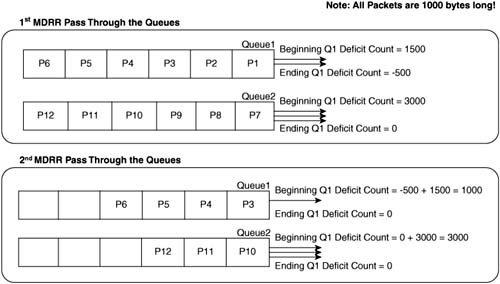
First, some extra information on how to interpret Figure 5-11 might help. The figure shows the action during the first round-robin pass in the top half of the figure, and the action during the second pass in the lower half of the figure. The example begins with six packets (labeled P1 through P6) in Queue 1, and six packets (labeled P7 through P12) in Queue 2. Each arrowed line, attached to the right sides of the queues, and pointing to the right, represents the choice by MDRR to send a single packet.
When a queue first fills, the queue’s deficit counter (DC) is set to the QV for that queue, which is 1500 for Queue 1, and 3000 for Queue 2. In Figure 5-11, MDRR begins by taking one packet from Queue 1, decrementing the DC to 500, and deciding that the DC has not been decremented to 0 (or less). MDRR takes a second packet from Queue 1, decrementing the DC to -500. MDRR then moves on to Queue 2, taking three packets, after which the DC for Queue 2 has decremented to 0.
That concludes the first round-robin pass through the queues. MDRR has taken 2000 bytes from Queue 1, and 3000 from Queue 2, giving the queues 40 percent and 60 percent of link bandwidth, respectively.
In the second round-robin pass, shown in the lower half of Figure 5-11, the process begins by MDRR adding the QV for each queue to the DC for each queue. Queue 1’s DC becomes 1500 + -500, or 1000, to begin the second pass. During this pass, MDRR takes P3 from Queue 1, decrements DC to 0, and then moves on to Queue 2. After taking three more packets from Queue 3, decrementing Queue 2’s DC to 0, MDRR completes the second pass. Over these two round-robin passes, MDRR has taken 3000 bytes from Queue 1, and 6000 from Queue 2—which is the same ratio as the ratio between the QVs.
With the deficit feature of MDRR, over time each queue receives a guaranteed bandwidth based on the following formula:
![]()
Note For additional examples of the operation of the MDRR deficit feature, refer to http://www.cisco.com/warp/public/63/toc_18841.html. Alternatively, you can go to www.cisco.com and search for “Understanding and Configuring MDRR and WRED on the Cisco 12000 Series Internet Router.”
The previous section explained four different types of queuing, focusing on the scheduler for each tool. Of those schedulers, one of the best features is the low latency treatment of packets in PQ’s high priority queue. Packets in PQ’s high queue always get serviced first, and spend very little time sitting in the queue. The other very useful scheduling feature was the capability to essentially reserve bandwidth for a particular queue with CQ or MDRR.
In this section, you will read about both the concepts and configuration for the three most commonly used Queuing tools in Cisco routers. CBWFQ uses a scheduler similar to CQ and MDRR, reserving link bandwidth for each queue. LLQ combines the bandwidth reservation feature of CBWFQ with a PQ-like high priority queue, called a Low Latency Queue, which allows delay-sensitive traffic to spend little time in the queue. But first, this section begins with WFQ, which uses a completely different scheduler.
Weighted Fair Queuing differs from PQ and CQ in several significant ways. The first and most obvious difference is that WFQ does not allow classification options to be configured! WFQ classifies packets based on flows. A flow consists of all packets that have the same source and destination IP address, and the same source and destination port numbers. So, no explicit matching is configured. The other large difference between WFQ versus PQ and CQ is the scheduler, which simply favors low-volume, higher-precedence flows over large-volume, lower-precedence flows. Also because WFQ is flow based, and each flow uses a different queue, the number of queues becomes rather large—up to a maximum of 4096 queues per interface. And although WFQ uses tail drop, it really uses a slightly modified tail-drop scheme—yet another difference.
Ironically, WFQ requires the least configuration of all the queuing tools in this chapter, yet it requires the most explanation to achieve a deep understanding. The extra work to read through the conceptual details will certainly help on the exam, plus it will give you a better appreciation for WFQ, which may be the most pervasively deployed QoS tool in Cisco routers.
Flow-Based WFQ, or just WFQ, classifies traffic into flows. Flows are identified by at least five items in an IP packet:
![]() Source IP address
Source IP address
![]() Destination IP address
Destination IP address
![]() Transport layer protocol (TCP or UDP) as defined by the IP Protocol header field
Transport layer protocol (TCP or UDP) as defined by the IP Protocol header field
![]() TCP or UDP source port
TCP or UDP source port
![]() TCP or UDP destination port
TCP or UDP destination port
![]() IP Precedence
IP Precedence
Depending on what document you read, WFQ also classifies based on the ToS byte, or more specifically, the IP Precedence field inside the ToS byte. Most documentation just lists the first five fields in the preceding list.
Whether WFQ uses the ToS byte or not when classifying packets, practically speaking, does not matter much. Good design suggests that packets in a single flow ought to have their Precedence or DSCP field set to the same value — so the same packets would get classified into the same flow, regardless of whether WFQ cares about the ToS byte or not for classification. (Regardless of whether you think of WFQ as classifying on ToS, or precedence, it is definitely true that the precedence of a packet impacts how the WFQ scheduler works.)
The term “flow” can have a couple of different meanings. For instance, imagine a PC that is downloading a web page. The user sees the page appear, reads the page for 10 seconds, and clicks a button. A second web page appears, the user reads the page for 10 seconds, and clicks another button. All the pages and objects came from a single web server, and all the pages and objects were loaded using a single TCP connection between the PC and the server. How many different combinations of source/destination, address/port, and transport layer protocol, are used? How many different flows?
From a commonsense perspective, only one flow exists in this example, because only one TCP connection is used. From WFQ’s perspective, no flows may have occurred, or three flows existed, and possibly even more. To most people, a single TCP flow exists as long as the TCP connection stays up, because the packets in that connection always have the same source address, source port, destination address, and destination port information. However, WFQ considers a flow to exist only as long as packets from that flow need to be enqueued. For instance, while the user is reading the web pages for 10 seconds, the routers finish sending all packets sent by the web server, so the queue for that flow is empty. Because the intermediate routers had no packets queued in the queue for that flow, WFQ removes the flow. Similarly, even while transferring different objects that comprise a web page, if WFQ empties a flow’s queue, it removes the queue, because it is no longer needed.
Why does it matter that flows come and go quickly from WFQ’s perspective? With class-based schemes, you always know how many queues you have, and you can see some basic statistics for each queue. With WFQ, the number of flows, and therefore the number of queues, changes very quickly. Although you can see statistics about active flows, you can bet on the information changing before you can type the show queue command again. The statistics show you information about the short-lived flow — for instance, when downloading the third web page in the previous example, the show queue command tells you about WFQ’s view of the flow, which may have begun when the third web page was being transferred, as opposed to when the TCP connection was formed.
Cisco publishes information about how the WFQ scheduler works. Even with an understanding of how the scheduler works, however, the true goals behind the scheduler are not obvious. This section reflects on what WFQ provides, and the following sections describe how WFQ accomplishes the task.
The WFQ scheduler has two main goals. The first is to provide fairness among the currently existing flows. To provide fairness, WFQ gives each flow an equal amount of bandwidth. If 10 flows exist for an interface, and the bandwidth is 128 kbps, each flow effectively gets 12.8 kbps. If 100 flows exist, each flow gets 1.28 kbps. In some ways, this goal is similar to a time-division multiplexing (TDM) system, but the number of time slots is not preset, but instead based on the number of flows currently exiting an interface. Also keep in mind that the concept of equal shares of bandwidth for each flow is a goal — for example, the actual scheduler logic used to accomplish this goal is much different from the bandwidth reservation using byte counts with CQ.
With each flow receiving its fair share of the link bandwidth, the lower-volume flows prosper, and the higher-volume flows suffer. Think of that 128-kbps link again, for instance, with 10 flows. If Flow 1 needs 5 kbps, and WFQ allows 12.8 kbps per flow, the queue associated with Flow 1 may never have more than a few packets in it, because the packets will drain quickly. If Flow 2 needs 30 kbps, then packets will back up in Flow 2’s queue, because WFQ only gives this queue 12.8 kbps as well. These packets experience more delay and jitter, and possibly loss if the queue fills. Of course, if Flow 1 only needs 5 kbps, the actual WFQ scheduler allows other flows to use the extra bandwidth.
The second goal of the WFQ scheduler is to provide more bandwidth to flows with higher IP precedence values. The preference of higher-precedence flows is implied in the name — “Weighted” implies that the fair share is weighted, and it is weighted based on precedence. With 10 flows on a 128-kbps link, for example, if 5 of the flows use precedence 0, and 5 use precedence 1, WFQ might want to give the precedence 1 flows twice as much bandwidth as the precedence 0 flows. Therefore, 5 precedence 0 flows would receive roughly 8.5 kbps each, and 5 precedence 1 flows would receive roughly 17 kbps each. In fact, WFQ provides a fair share roughly based on the ratio of each flow’s precedence, plus one. In other words, precedence 7 flows get 8 times more bandwidth than does precedence 0 flows, because (7 + 1) / (0 + 1) = 8. If you compare precedence 3 to precedence 0, the ratio is roughly (3 + 1) / (0 + 1) = 4.
So, what does WFQ accomplish? Ignoring precedence for a moment, the short answer is lower-volume flows get relatively better service, and higher-volume flows get worse service. Higher-precedence flows get better service than lower-precedence flows. If lower-volume flows are given higher-precedence values, the bandwidth/delay/jitter/loss characteristics improve even more.
In a network where most of the delay-sensitive traffic is lower-volume traffic, WFQ is a great solution. It takes one command to enable it, and it is already enabled by default! Its default behavior favors lower-volume flows, which may be the more important flows. In fact, WFQ came out when many networks’ most important interactive flows were Telnet and Systems Network Architecture (SNA) encapsulated in IP. These types of flows used much less volume than other flows, so WFQ provided a great default, without having to worry about how to perform prioritization on encapsulated SNA traffic.
WFQ gives each flow a weighted percentage of link bandwidth. However, WFQ does not predefine queues like class-based queuing tools do, because WFQ dynamically creates queues to hold the packets in each flow. And although WFQ ends up causing each flow to get some percentage of link bandwidth, the percentage changes, and changes rapidly, because flows come and go frequently. Because each flow may have different precedence values, the percentage of link bandwidth for each flow will change, and it will change very quickly, as each flow is added or removed. In short, WFQ simply could not be implemented by assigning a percentage of bandwidth, or a byte count, to each queue.
The WFQ scheduler is actually very simple. When the Hardware Queue frees a slot, WFQ can move one packet to the Hardware Queue, just like any other queuing tool. The WFQ scheduler takes the packet with the lowest sequence number (SN) among all the queues, and moves it to the Hardware Queue. The SN is assigned when the packet is placed into a queue, which is where the interesting part of WFQ scheduling takes place.
Caution The Cisco QoS course uses the term “Finish Time” (FT) instead of Sequence Number, but its usage is identical to the coverage shown here. You should be aware of both terms for the exam.
For perspective on the sequence of events, marking the SN, and serving the queues, examine Figure 5-12.
WFQ calculates the SN before adding a packet to its associated queue. In fact, WFQ calculates the SN before making the drop decision, because the SN is part of the modified tail-drop logic. The WFQ scheduler considers both packet length and precedence when calculating the SN. The formula for calculating the SN for a packet is as follows:
![]()
Where “weight” is calculated as follows:
![]()
The formula considers the length of the new packet, the weight of the flow, and the previous SN. By considering the packet length, the SN calculation results in a higher number for larger packets, and a lower number for smaller packets. The formula considers the SN of the most recently enqueued packet in the queue for the new sequence number. By including the SN of the previous packet enqueued into that queue, the formula assigns a larger number for packets in queues that already have a larger number of packets enqueued.
The third component of the formula, the weight, is the most interesting part. The WFQ scheduler sends the packet with the lowest SN next, and WFQ wants to give more bandwidth to the higher-precedence flows. So, the weight values are inversely proportional to the precedence values. Table 5-5 lists the weight values used by WFQ as of 12.0(5)T/12.1.

As seen in the table, the larger the precedence value, the lower the weight, in turn making the SN lower. An example certainly helps for a fuller understanding. Consider the example in Figure 5-13, which illustrates one existing flow and one new flow.

When adding new packet 1 to the queue for Flow 1, WFQ just runs the formula against the length of the new packet (100) and the weight, adding the SN of the last packet in the queue to which the new packet will be added. For new flows, the same formula is used; because there are no other packets in the queue, however, the SN of the most recently sent packet, in this case 100, is used in the formula. In either case, WFQ assigns larger SN values for larger packets and for those with lower IP precedence.
A more detailed example can show some of the effects of the WFQ SN assignment algorithm and how it achieves its basic goals. Figure 5-14 shows a set of four flow queues, each with four packets of varying lengths. For the sake of discussion, assume that the SN of the previously sent packet is zero in this case. Each flow’s first packet arrives at the same instant in time, and all packets for all flows arrive before any more packets can be taken from the WFQ queues.

In this example, each flow had four packets arrive, all with a precedence of zero. The packets in Flow 1 were all 1500 bytes in length; in Flow 2, the packets were 1000 bytes in length; in Flow 3, they were 500 bytes; and finally, in Flow 4, they were 100 bytes. With equal precedence values, the Flow 4 packets should get better service, because the packets are much smaller. In fact, all four of Flow 4’s packets would be serviced before any of the packets in the other flows. Flow 3’s packets are sent before most of the packets in Flow 1 and Flow 2. Thus, the goal of giving the lower-volume flows better service is accomplished, assuming the precedence values are equal.
Note For the record, the order the packets would exit the interface, assuming no other events occur, is 13 first, then 14, followed by 15, 16, 9, 5, 10, 1, 11, 6, 12, 2, 7, 8, 3, 4.
To see the effect of different precedence values, look at Figure 5-15, which lists the same basic scenario but with varying precedence values.

The SNs for Flow 1 and Flow 2 improve dramatically with the higher precedence values of 3 and 5, respectively. Flow 4 still gets relatively good service, even at precedence 0. Two packets from Flow 2, and one from Flow 1, will be serviced before Flow 4’s fourth packet (SN 12,953,600), which is an example of how the higher precedence value gives the packets in this flow slightly better service. So, the lower-volume, but lower-precedence flows will have some degradation in service relative to the higher-volume, but higher-precedence flows.
Note For the record, the order the packets would exit the interface, assuming no other events occur, is 13, 5, 14, 15, 6, 1, 16, 7, 9, 8, 2, 10, 3, 4, 11, 12.
Finally, a router using WFQ can experience a phenomenon called too fair. With many flows, WFQ will give some bandwidth to every flow. In the previous example, what happens if 200 new flows begin? Each of those new flows will get a relatively low SN, because the SN of the most recently sent packet is used in the formula. The packets that are already in the existing queues will have to wait on all the new packets. In an effort to give each flow some of the link bandwidth, WFQ may actually not give some or most of the flows enough bandwidth for them to survive.
WFQ uses a slightly modified tail-drop policy for choosing when to drop packets. The decision is based on several factors, one being the SN of the packet.
WFQ places an absolute limit on the number of packets enqueued among all queues; this value is called the hold-queue limit. If a new packet arrives, and the hold-queue limit has been reached, the packet is discarded. That part of the decision is based not on a single queue, but on the whole WFQ queuing system for the interface.
The next decision is based on an individual queue. If a packet needs to be placed into a queue, and that queue’s congestive discard threshold (CDT) has been reached, the packet may be thrown away. CDT is a little like a maximum queue length for each flow’s queue, but WFQ puts a little twist on how the concept is used (hence the use of another term, instead of just calling it the maximum queue length). To appreciate how the CDT is used, examine Figure 5-16.

The hold-queue size limits the total number of packets in all of the flow or conversation queues. However, CDT limits the number of packets in each individual queue. If CDT packets are already in the queue into which a packet should be placed, WFQ considers discarding the new packet. Normally, the new packet is discarded. If a packet with a larger SN has already been enqueued in a different queue, however, WFQ instead discards the packet with the larger SN! It’s like going to Disneyland, getting in line, and then being told that a bunch of VIPs showed up, so you cannot ride the ride, and you will have to come back later. (Hopefully Disney would not take you out of the line and send you to the bit bucket, though!) In short, WFQ can discard a packet in another flow when the queue for a different flow has exceeded CDT but still has lower sequence numbers. You can configure the CDT to a value between 1 and 4096, inclusive.
Finally, WFQ can be configured for a maximum of 4096 queues, but interestingly, the actual value can only be a power of 2 between 16 and 4096, inclusive. The IOS restricts the values because WFQ performs a hash algorithm to classify traffic, and the hash algorithm only works when the number of queues is one of these valid values.
Although you do not really need to know much detail for the QOS exam, there are a couple of types of WFQ queues about which you should at least be aware. First, WFQ keeps eight hidden queues for overhead traffic generated by the router. WFQ uses a very low weight for these queues in order to give preference to the overhead traffic.
The other type of queue isn’t really hidden, but most people simply don’t notice them. You can configure RSVP on the same interface as WFQ. As you might recall from Chapter 2, “QoS Tools and Architectures,” RSVP reserves bandwidth on an interface. To reserve the bandwidth, RSVP asks WFQ to create a queue for each RSVP-reserved flow, and to give it a very low weight. As you will read in the next section, you can configure WFQ for the number of concurrent RSVP queues that can be used on an interface.
Although WFQ requires a little deeper examination to understand all the underlying concepts, configuration is simple. IOS uses WFQ by default on all serial interfaces with bandwidths set at T/1 and E/1 speeds and below. None of WFQ’s parameters can be set for an individual queue, so at most, the WFQ configuration will be one or two lines long. An example configuration for WFQ follows Tables 5-6 and 5-7. Tables 5-6 and 5-7 list the configuration and exec commands related to WFQ respectively.


In the next example, R3 uses WFQ on its S0/0 interface. R3 marks the packets as they enter E0/0, using CB marking. Two voice calls, plus one FTP download, and a large web page download generate the traffic. The web page is the same one used throughout the book, with competing frames on the left and right side of the page. Note that each of the two frames in the web page uses two separate TCP connections. The marking logic performed by CB marking is as follows:
![]() VoIP payload—DSCP EF
VoIP payload—DSCP EF
![]() HTTP traffic for web pages with “important” in the URL—DSCP AF21
HTTP traffic for web pages with “important” in the URL—DSCP AF21
![]() HTTP traffic for web pages with “not” in the URL—DSCP AF23
HTTP traffic for web pages with “not” in the URL—DSCP AF23
![]() All other—DSCP BE
All other—DSCP BE
Repetitive examples do not help much with WFQ, because there is little to configure. Example 5-3 shows the basic configuration, followed by some show commands. After that, it shows a few of the optional parameters being set. The example uses the familiar network diagram, as repeated in Figure 5-17.

Example 5-3 WFQ Configuration and show Commands
Enter configuration commands, one per line. End with CNTL/Z.
R3(config)#int s 0/0
R3(config-if)#fair-queue
R3(config-if)#^Z
R3#sh int s 0/0
Serial0/0 is up, line protocol is up
Hardware is PowerQUICC Serial
Description: connected to FRS port S0. Single PVC to R1.
MTU 1500 bytes, BW 1544 Kbit, DLY 20000 usec,
reliability 255/255, txload 9/255, rxload 8/255
Encapsulation FRAME-RELAY, loopback not set
Keepalive set (10 sec)
LMI enq sent 171, LMI stat recvd 163, LMI upd recvd 0, DTE LMI up
LMI enq recvd 0, LMI stat sent 0, LMI upd sent 0
LMI DLCI 1023 LMI type is CISCO frame relay DTE
Broadcast queue 0/64, broadcasts sent/dropped 378/2, interface broadcasts 347
Last input 00:00:01, output 00:00:00, output hang never
Last clearing of "show interface" counters 00:28:46
Input queue: 0/75/0/0 (size/max/drops/flushes); Total output drops: 8249
Output queue: 126/1000/64/8249 (size/max total/threshold/drops)
Conversations 6/7/256 (active/max active/max total)
Reserved Conversations 0/0 (allocated/max allocated)
5 minute input rate 52000 bits/sec, 97 packets/sec
5 minute output rate 58000 bits/sec, 78 packets/sec
36509 packets input, 2347716 bytes, 0 no buffer
Received 0 broadcasts, 0 runts, 0 giants, 0 throttles
1 input errors, 0 CRC, 1 frame, 0 overrun, 0 ignored, 0 abort
28212 packets output, 2623792 bytes, 0 underruns
0 output errors, 0 collisions, 5 interface resets
0 output buffer failures, 0 output buffers swapped out
10 carrier transitions
DCD=up DSR=up DTR=up RTS=up CTS=up
R3#show queueing fair
Current fair queue configuration:
Interface Discard Dynamic Reserved Link Priority
threshold queues queues queues queues
Serial0/0 64 256 0 8 1
Serial0/1 64 256 0 8 1
R3#show queueing fair int s 0/0
Current fair queue configuration:
Interface Discard Dynamic Reserved Link Priority
threshold queues queues queues queues
Serial0/0 64 256 0 8 1
R3# show queue s 0/0
Queueing strategy: weighted fair
Output queue: 79/1000/64/11027 (size/max total/threshold/drops)
Conversations 4/8/256 (active/max active/max total)
Reserved Conversations 0/0 (allocated/max allocated)
Available Bandwidth 1158 kilobits/sec
(depth/weight/total drops/no-buffer drops/interleaves) 37/5397/1359/0/0
Conversation 15, linktype: ip, length: 64
source: 192.168.3.254, destination: 192.168.2.251, id: 0x013B, ttl: 253,
TOS: 184 prot: 17, source port 16772, destination port 19232
! Next stanza lists info about one of the VoIP calls
Conversation 125, linktype: ip, length: 64
source: 192.168.3.254, destination: 192.168.2.251, id: 0x0134, ttl: 253,
Conversation 33, linktype: ip, length: 1404
source: 192.168.3.100, destination: 192.168.1.100, id: 0xFF50, ttl: 127,
Conversation 34, linktype: ip, length: 1404
source: 192.168.3.100, destination: 192.168.1.100, id: 0xFF53, ttl: 127,
R3#configure terminal
Enter configuration commands, one per line. End with CNTL/Z.
R3(config)#int s 0/0
R3(config-if)#fair-queue 100 64 10
R3(config-if)#hold-queue 500 out
R3(config-if)#^Z
!
R3#show interface serial 0/0
Serial0/0 is up, line protocol is up
Hardware is PowerQUICC Serial
Description: connected to FRS port S0. Single PVC to R1.
MTU 1500 bytes, BW 1544 Kbit, DLY 20000 usec,
reliability 255/255, txload 9/255, rxload 8/255
Encapsulation FRAME-RELAY, loopback not set
Keepalive set (10 sec)
LMI enq sent 198, LMI stat recvd 190, LMI upd recvd 0, DTE LMI up
LMI enq recvd 0, LMI stat sent 0, LMI upd sent 0
LMI DLCI 1023 LMI type is CISCO frame relay DTE
Broadcast queue 0/64, broadcasts sent/dropped 442/2, interface broadcasts 406
Last input 00:00:01, output 00:00:00, output hang never
Last clearing of "show interface" counters 00:33:14
Input queue: 0/75/0/0 (size/max/drops/flushes); Total output drops: 12474
Output queue: 95/500/100/12474 (size/max total/threshold/drops)
Conversations 5/6/64 (active/max active/max total)
Available Bandwidth 1158 kilobits/sec
! lines omitted for brevity
R3#show queueing fair
Interface Discard Dynamic Reserved Link Priority
threshold queues queues queues queues
Serial0/1 64 256 0 8 1
Input queue: 0/75/0/0 (size/max/drops/flushes); Total output drops: 13567
Output queue: 125/500/100/13567 (size/max total/threshold/drops)
Conversations 5/7/64 (active/max active/max total)
Reserved Conversations 0/0 (allocated/max allocated)
Available Bandwidth 1158 kilobits/sec
(depth/weight/total drops/no-buffer drops/interleaves) 61/5397/654/0/0
Conversation 61, linktype: ip, length: 64
source: 192.168.3.254, destination: 192.168.2.251, id: 0x0134, ttl: 253,
TOS: 184 prot: 17, source port 16638, destination port 19476
(depth/weight/total drops/no-buffer drops/interleaves) 61/5397/653/0/0
Conversation 15, linktype: ip, length: 64
source: 192.168.3.254, destination: 192.168.2.251, id: 0x013B, ttl: 253,
TOS: 184 prot: 17, source port 16772, destination port 19232
(depth/weight/total drops/no-buffer drops/interleaves) 1/10794/15/0/0
Conversation 34, linktype: ip, length: 1404
source: 192.168.3.100, destination: 192.168.1.100, id: 0x00A5, ttl: 127,
TOS: 88 prot: 6, source port 80, destination port 1068
(depth/weight/total drops/no-buffer drops/interleaves) 1/10794/15/0/0
Conversation 33, linktype: ip, length: 1404
source: 192.168.3.100, destination: 192.168.1.100, id: 0x00A7, ttl: 127,
TOS: 72 prot: 6, source port 80, destination port 1067
(depth/weight/total drops/no-buffer drops/interleaves) 1/32384/12/0/0
Conversation 29, linktype: ip, length: 1404
source: 192.168.3.100, destination: 192.168.1.100, id: 0x00A1, ttl: 127,
TOS: 0 prot: 6, source port 1353, destination port 1065
To enable WFQ, the fair-queue interface subcommand is used. After enabling WFQ, the show interface command output shows the fact that WFQ is enabled. (See the highlighted portion of the first show interface command in Example 5-3.) Note that the hold queue default size of 1000 is shown in the show interface output as well. The show interface command and the show queueing fair commands both list the CDT (default 64), along with the maximum number of queues (256).
The most interesting show command for WFQ is the show queue command. Note that a summary section is listed first, followed by a stanza of output for each active flow. Each stanza lists statistics about the current queue size, number of drops, and so on. Each stanza also lists the details used for classification. For instance, each stanza of the first show queue command includes a comment added by me. Knowing that two voice calls, one TCP connection for FTP, and two TCP connections for HTTP were being used, I could look at the source and destination addresses and ports numbers and decide which WFQ flows correlated to each of these user flows.
You can understand the usage of the ToS byte by WFQ with a little closer examination of the output of the show queue command. You may recall that the two HTTP transfers were marked with different DSCP values; note that the two HTTP flows in the command output have ToS byte values of 72 and 80. Which of these values corresponds to DSCP AF21 (important HTTP URLs per CB marking) and AF23 (“not” important URLs per CB marking)? Table 5-8 lists the pertinent details needed to correlate DSCP, ToS, and precedence values used in the example.
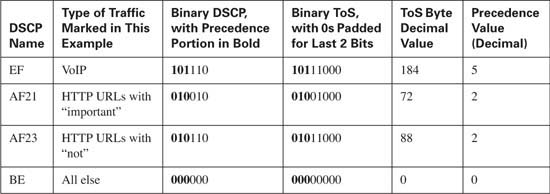
WFQ always weights the packets based on the first 3 bits of the ToS byte — in other words, based on the Precedence field. However, the show queue command output lists the entire contents of the ToS byte, which in this case included 6 bits marked by CB marking, and two trailing binary 0s. Therefore, the ToS byte values in the command lists the same values shown in the table. Even though CB marking marked a different DSCP for each type of HTTP traffic, as far as WFQ is concerned, each receives the same amount of weight. This is because WFQ does not look past the Precedence field when determining the weight.
Finally, the second half of Example 5-3 just shows some configuration changes and the resulting changes in the show command output. The configuration changes the CDT, the maximum number of queues, and the length of the hold queue. The highlighted portions of the show interface, show queueing, and show queue commands reflect the details of the configuration changes.
WFQ works well for networks where the most delay-sensitive traffic requires less bandwidth than the average flow. Also flows with higher precedence work well, with low-volume, high-precedence flows receiving exceptional treatment. Best of all, WFQ requires no classification configuration. As a result, WFQ provides a great default queuing choice, particularly when traffic characteristics are unpredictable and difficult to qualify.
WFQ works poorly for voice and interactive video traffic, because both need low delay and low jitter. WFQ does not provide a priority queue in order to minimize delay and jitter. Also delay can increase when too many concurrent flows occur, due to WFQ being “too fair,” allowing some bandwidth to each flow, which may cause the voice or video flows to not get enough bandwidth.
Table 5-9 summarizes some of the key features of WFQ.
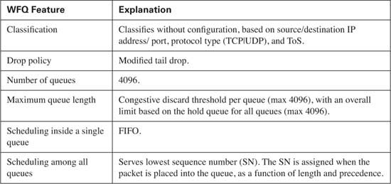
Of the other Queuing tools covered in this chapter, CBWFQ is most like CQ, in that it can be used to reserve minimum bandwidth for each queue. It does differ from CQ in that you can configure the actual percentage of traffic, rather than a byte count. CBWFQ is like WFQ in that CBWFQ can actually use WFQ inside one particular queue, but it differs from WFQ in that it does not keep up with flows for all the traffic.
To begin the coverage of CBWFQ, examine Figure 5-18, which outlines the typical queuing features in sequence.

Starting left to right in the figure, CBWFQ classifies packets using the exact same set of fields that CB marking uses to classify packets. In fact, CBWFQ uses the exact same configuration commands, all of which are part of the Modular QoS CLI (MQC) commands described in Chapter 3, “MQC, QPM, and AutoQoS.” CBWFQ’s use of MQC makes learning the configuration for CBWFQ easy, assuming you remember how to configure CB marking from the preceding chapter. And unlike WFQ, which use flow-based classifiers, CBWFQ does not classify based on the flow, but on anything you can match with the MQC commands.
Note CBWFQ uses the terms “class” and “queue” to refer to the single queue that is associated with a class that can be defined with CBWFQ. The terms “class” and “queue” are often used interchangeably when describing CBWFQ.
CBWFQ supports two types of drop policy, namely tail drop and WRED. Chapter 7, “Congestion Avoidance Through Drop Policies,” covers WRED in detail, but the general idea is to discard packets before the queue actually fills, with the intent of making some TCP connections react to the lost packet and slow down sending packets. By having a few TCP connections slow down, the queue may not fill, reducing congestion.
You can enable WRED on any of the 64 queues available with CBWFQ. However, WRED is a good option for some queues, and not for others. If a queue holds on to VoIP payload, for example, you do not really want to drop any packets, because if you drop voice packets, the voice quality degrades. In queues holding less-drop-sensitive traffic, such as data, WRED is a good option, but WRED works poorly in queues holding voice and video traffic.
CBWFQ supports 64 queues, with a maximum and default queue length varying depending on the model of router and the amount of memory installed. All 64 queues can be configured, but one class queue, called class-default, is automatically configured. If the explicitly configured classification does not match a packet, IOS places the packet into the class-default class. You are allowed to change the configuration details regarding this default class, but this one class always exists.
So far, the other queuing tools in this chapter supported only FIFO logic inside a single queue. In fact, some of you may have been wondering why “step 5” was included in illustrations such as the one shown in Figure 5-19. Currently, CBWFQ can use either FIFO or WFQ inside the class-default queue. With Flow-Based WFQ in the class-default queue, when CBWFQ decides to take one or more packets from the queue, it takes the packet with the best sequence number (SN) — just like WFQ normally does.

Note Cisco 7500 series routers support either FIFO or WFQ inside each and every CBWFQ queue, whereas other platforms only support both FIFO and WFQ inside CBWFQ’s class-default queue.
CBWFQ provides a great advantage by allowing WFQ to be used in the class-default queue. You may recall that WFQ is actually a very good default choice for queuing, because it treats low-volume flows well, and many low-volume flows are also interactive flows. WFQ also treats packets with high precedence well. So, with CBWFQ, for the traffic you know about, you classify it, and reserve the right amount of bandwidth for the class. For the traffic you cannot characterize, you let it default into the class-default queue, where you can dynamically apply some fairness to the default traffic by using WFQ. The capability to reserve bandwidth for some packets, and fairly assign the rest of the bandwidth with WFQ, makes CBWFQ a very powerful queuing tool.
Finally, Cisco does tell us the general idea behind how the CBWFQ scheduler works. The scheduler gives a percentage of the bandwidth to each class, based on the configured values. For instance, four classes, including class-default, may be configured with bandwidth percentages that total 100 percent. The scheduler ensures that each queue receives that percentage of bandwidth. If some queues do not need their bandwidth for a short period, the bandwidth is spread across the other classes. Cisco does not really offer more details about how the scheduler works—so you do not need to worry more about how CBWFQ works for the exams!
Table 5-8 summarizes some of the key features of CBWFQ.
Table 5-8 CBWFQ Functions and Features

* Except on 7500 series, where you can use FIFO or WFQ in all the CBWFQ queues.
CBWFQ configuration uses many of the same MQC commands as covered in Chapter 3 and Chapter 4. As a result, CBWFQ configuration should be relatively easy to understand. The commands used for CBWFQ configuration are listed Tables 5-11 and 5-12.
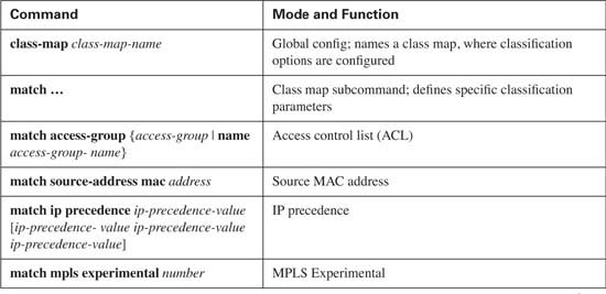
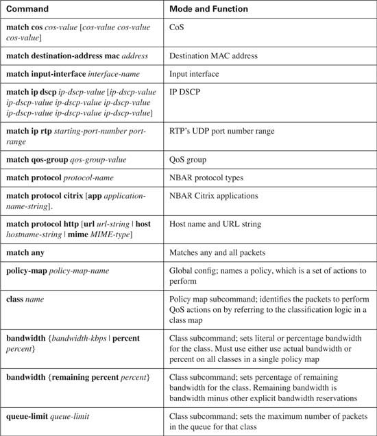
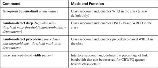
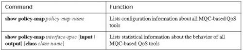
The remainder of this section includes several familiar lab scenarios, with example configurations and show commands. In the first CBWFQ example, R3 uses CBWFQ on its S0/0 interface. The engineer configuring R3 decided that voice traffic could benefit from being placed into a different queue than all other traffic, so a simple QoS policy has been devised, which includes the following:
![]() All VoIP payload traffic is placed in a queue.
All VoIP payload traffic is placed in a queue.
![]() All other traffic is placed in another queue.
All other traffic is placed in another queue.
![]() Give the VoIP traffic 50 percent of the bandwidth.
Give the VoIP traffic 50 percent of the bandwidth.
![]() WFQ and WRED should be used on the non-VoIP traffic.
WFQ and WRED should be used on the non-VoIP traffic.
Figure 5-19 reminds you of the now-familiar example network, which shows the router in which the configuration is applied. Example 5-4 shows the configuration and show commands.
Example 5-4 CBWFQ, VoIP in High Queue, Everything Else in Normal Queue
Building configuration...
match ip rtp 16384 16383
class voip-rtp
bandwidth percent 50
class class-default
fair-queue
!
interface Serial0/0
description connected to FRS port S0. Single PVC to R1.
no ip address
encapsulation frame-relay
bandwidth 128
service-policy output queue-voip
!
interface Serial0/0.1 point-to-point
description point-point subint global DLCI 103, connected via PVC to DLCI 101 (
ip address 192.168.2.253 255.255.255.0
frame-relay interface-dlci 101
! Portions omitted for brevity
R3#show policy-map int s 0/0
Serial0/0
Service-policy output: queue-voip
30 second offered rate 51000 bps, drop rate 0 bps
Match: ip rtp 16384 16383
Weighted Fair Queueing
Output Queue: Conversation 265
(depth/total drops/no-buffer drops) 14/0/0
Weighted Fair Queueing
Flow Based Fair Queueing
Maximum Number of Hashed Queues 256
R3#show policy-map int s 0/0 output class class-default Serial0/0
Service-policy output: queue-voip
Class-map: class-default (match-any)
2217 packets, 1417985 bytes
30 second offered rate 71000 bps, drop rate 0 bps
Match: any
Weighted Fair Queueing
Flow Based Fair Queueing
Maximum Number of Hashed Queues 256
(total queued/total drops/no-buffer drops) 10/0/0
R3#show policy-map
Class voip-rtp
Weighted Fair Queueing
Class class-default
Flow based Fair Queueing Max Threshold 64 (packets)
R3#show interface s 0/0
Serial0/0 is up, line protocol is up
Hardware is PowerQUICC Serial
Description: connected to FRS port S0. Single PVC to R1.
MTU 1500 bytes, BW 1544 Kbit, DLY 20000 usec,
reliability 255/255, txload 9/255, rxload 8/255
Encapsulation FRAME-RELAY, loopback not set
Keepalive set (10 sec)
LMI enq sent 132, LMI stat recvd 132, LMI upd recvd 0, DTE LMI up
LMI enq recvd 0, LMI stat sent 0, LMI upd sent 0
LMI DLCI 1023 LMI type is CISCO frame relay DTE
FR SVC disabled, LAPF state down
Broadcast queue 0/64, broadcasts sent/dropped 307/0, interface broadcasts 285
Last input 00:00:02, output 00:00:00, output hang never
Last clearing of "show interface" counters 00:22:02
Input queue: 0/75/0/0 (size/max/drops/flushes); Total output drops: 0
Output queue: 16/1000/64/0 (size/max total/threshold/drops)
Reserved Conversations 1/1 (allocated/max allocated)
Available Bandwidth 1158 kilobits/sec
30 second input rate 52000 bits/sec, 102 packets/sec
30 second output rate 59000 bits/sec, 101 packets/sec
126301 packets input, 8141304 bytes, 0 no buffer
Received 0 broadcasts, 0 runts, 0 giants, 0 throttles
0 input errors, 0 CRC, 0 frame, 0 overrun, 0 ignored, 0 abort
126197 packets output, 8550371 bytes, 0 underruns
0 output errors, 0 collisions, 2 interface resets
0 output buffer failures, 0 output buffers swapped out
0 carrier transitions
DCD=up DSR=up DTR=up RTS=up CTS=up
R3#configure terminal
Enter configuration commands, one per line. End with CNTL/Z.
R3(config)#policy-map queue-voip
R3(config-pmap)#class class-default
R3(config-pmap-c)#no fair-queue
R3(config-pmap-c)#^Z
R3#show policy-map
Policy Map queue-voip
Class voip-rtp
Weighted Fair Queueing
Bandwidth 50 (%) Max Threshold 64 (packets)
The configuration for CBWFQ requires many commands, but the logic is straightforward. class-map voip-rtp matches all VoIP payload by matching with the match ip rtp 16384 16383 command. The policy-map queue-voip policy assigns VoIP traffic 50 percent of the bandwidth based on the bandwidth percent 50 command. But 50 percent of what? Well, the actual bandwidth is derived from the percentage of the bandwidth configured on the bandwidth interface subcommand. In this case, the bandwidth is set to 128, so the voip-rtp class gets 64 kbps, which is enough for the two G.729a VoIP calls. Just like with CB marking, the service-policy output command enables the policy on the interface, in this case S0/0.
The show policy-map interface serial 0/0 command lists the most interesting statistical information about CBWFQ. (This paragraph, and the rest of the text that describes Example 5-4, explains the commands in the example in the same sequence as they are shown in the example.) It lists a stanza of information for each class, listing the configured matching parameters and bandwidth percentages. The offered rate of traffic that has been classified into each queue is listed, along with drop statistics. These values are useful when monitoring the configuration to decide whether the configuration values should be changed. Also note that in class-default, the output implies that Flow-Based WFQ is in use inside the queue.
The show policy-map command also has other options that reduce the amount of output, which can be large. For instance, the show policy-map int s 0/0 output class class-default shown in the example lists only information about class class-default.
The show policy-map command just lists a summary of the configured policy maps. Interestingly, the class-default stanza of the command output lists Weighted Fair Queuing, and then says it is “flow based.” In this case, the command output is reminding you that inside the class-default queue, Flow-Based WFQ is applied to each flow. For comparison, at the end of the example, the configuration has been changed to disable WFQ in the class-default queue. The show policy-map command no longer lists Flow-Based WFQ for class-default.
Although some of the CBWFQ command output references WFQ in sections describing queues other than class-default, CBWFQ does not use Flow-Based WFQ inside any of these queues. CBWFQ on most Cisco router models can only use Flow-Based WFQ inside one queue—the class-default queue. (On the 7500, WFQ can be used inside each CBWFQ queue.)
Good QoS design calls for the marking of packets close to the source of the packet. Example 5-5 accomplishes the same queuing goals as the preceding example, but CBWFQ relies on the fact that the packets have been marked before reaching R3’s S0/0 interface. In a real network, the packets could be marked on one of the LAN switches, or in an IP Phone, or by the computers in the network.
This example shows the packets being marked upon entering R3’s E0/0 interface, just like Example 4-1 in Chapter 4. Example 5-5 shows the revised configuration based on the following criteria:
![]() All VoIP payload traffic has been marked with DSCP EF; place this traffic in a queue.
All VoIP payload traffic has been marked with DSCP EF; place this traffic in a queue.
![]() All other traffic has been marked with DSCP BE; place this traffic in a different queue.
All other traffic has been marked with DSCP BE; place this traffic in a different queue.
![]() Give the VoIP traffic 58 kbps of the bandwidth on the link.
Give the VoIP traffic 58 kbps of the bandwidth on the link.
![]() Use WRED and WFQ on the non-VoIP traffic.
Use WRED and WFQ on the non-VoIP traffic.
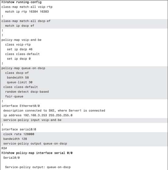
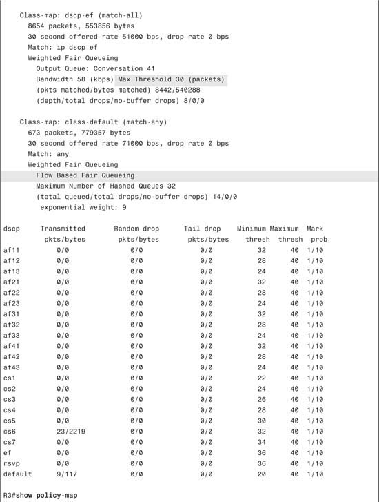

The configuration is again detailed, but straightforward. policy-map voip-and-be marks packets as they enter E0/0, matching and marking VoIP packets with DSCP EF, and matching and marking all other packets, marking them with DSCP BE. The class-map match-all dscp-ef command creates a class that matches all DSCP EF traffic. policy-map queue-on-dscp refers to class dscp-ef in order to match all VoIP traffic, giving the voice traffic 58 kbps with the bandwidth 58 command. That same class includes the queue-limit 30 command, which changes the maximum queue size to 30. CBWFQ uses tail drop in each class by default, so under the class class-default command, the random-detect dscp-based command is used to enable WRED in the default class. In addition, of course, the service-policy command enables the service policy on the interface.
The show commands do not provide much new information, other than the statistics about WRED operation. The details about this part of the output are covered in Chapter 6.
You may have found it strange to see a configuration with classification and marking happening as the packet entered E0/0 in R3, and then another round of classification for packets exiting R3’s S0/ 0 interface. One of the great advantages of classification and marking is that after the packets are marked, the configuration of the tools providing each per-hop behavior (PHB) is simple. Another advantage is that after the packet has been marked, other devices can perform the simpler matching of just looking for DSCP or IP precedence.
If the QoS policy calls for applying PHBs only for packets exiting WAN interfaces, and the policy does not call for PHBs between packets entering and exiting LAN interfaces, the classification and marking, and the queuing, may be performed with a single configuration. Example 5-6 shows a similar configuration to the preceding example, but with both the marking and queuing performed for packets exiting R3’s S0/0 interface.
Example 5-6 CBWFQ and CB Marking Combined
class-map match-all voip-rtp
match ip rtp 16384 16383
!
policy-map mark-and-queue
class voip-rtp
bandwidth 58
fair-queue
!
interface Ethernet0/0
description connected to SW2, where Server1 is connected
interface serial0/0
clock rate 128000
bandwidth 128
Two classes are used in this example: voip-rtp, which matches all VoIP payload UDP ports; and class-default, which matches all other packets. Inside policy-map mark-and-queue, each class includes a set command to set the DSCP value. The voip-rtp class includes a bandwidth command to reserve bandwidth; class-default automatically gets 25 percent of the bandwidth. The service-policy output mark-and-queue command enables the policy for packets exiting R3’s S0/0 interface. In this example, you get the benefits of classification and marking, a shorter configuration, and only one classification step inside this router, reducing overhead.
CBWFQ provides several variations of how to configure the bandwidth reserved for each queue. For instance, the bandwidth 64 class subcommand reserves 64 kbps of bandwidth, regardless of the bandwidth setting on the interface. The bandwidth percent 25 class subcommand would also reserve 64 kbps for a class if the interface bandwidth had been set to 256 kbps, using the bandwidth 256 interface subcommand.
Both styles of the bandwidth commands do the same thing in this case, but which is better? Well, if your intent is to truly give a particular queue 25 percent of the bandwidth, regardless of the actual bandwidth, use the percent option. That way, if you actually increase the speed of the link in the future, all you have to do is change the setting for the bandwidth interface subcommand to reflect the increased bandwidth into CBWFQ. However, if you specifically engineer a queue to use a set amount of bandwidth, and that bandwidth requirement should not be increased even if the link speed increases, then use the bandwidth class subcommand without the percent option.
Example 5-7 shows these two variations on the bandwidth class subcommand, along with a few caveats.
Example 5-7 Use of the Bandwidth Command, with and without the Percent Option
Enter configuration commands, one per line. End with CNTL/Z.
R3(config)#class-map class1
R3(config-cmap)#match ip dscp af31
R3(config-cmap)#class-map class2
R3(config-cmap)#match ip dscp af32
R3(config-cmap)#class-map class3
R3(config-cmap)#match ip dscp af33
R3(config-cmap)#class-map class4
R3(config-cmap)#match ip dscp af21
R3(config-cmap)#policy-map explicit-bw
R3(config-pmap)#class class1
R3(config-pmap-c)#bandwidth 64
R3(config-pmap-c)#class class2
R3(config-pmap-c)#bandwidth percent 25
All classes with bandwidth should have consistent units
R3(config-pmap-c)#bandwidth 32
!
R3(config-pmap-c)#policy-map percent-bw
R3(config-pmap)#class class3
R3(config-pmap-c)#bandwidth percent 25
R3(config-pmap-c)#class class4
R3(config-pmap-c)#bandwidth 64
All classes with bandwidth should have consistent units
R3(config-pmap-c)#bandwidth percent 25
R3(config-pmap-c)#int s 0/1
R3(config-if)#bandwidth 64
R3(config-if)#service-policy output explicit-bw
I/f Serial0/1 class class1 requested bandwidth 64 (kbps), available only 48 (kbps)
R3(config-if)#service-policy output percent-bw
R3(config-if)#^Z
R3#show running-config
00:05:05: %SYS-5-CONFIG_I: Configured from console by console
Building configuration...
! Portions omitted for brevity
!
class-map match-all class4
match ip dscp af21
class-map match-all class3
match ip dscp af33
class-map match-all class2
match ip dscp af32
class-map match-all class1
match ip dscp af31
!
policy-map explicit-bw
class class1
bandwidth 64
class class2
bandwidth 32
!
policy-map percent-bw
class class3
bandwidth percent 25
class class4
bandwidth percent 25
!
R3#show policy-map interface s 0/1
Serial0/1
Service-policy output: percent-bw
Class-map: class3 (match-all)
5 minute offered rate 0 bps, drop rate 0 bps
Match: ip dscp af33
Queueing
Output Queue: Conversation 25
Bandwidth 25 (%)
Bandwidth 16 (kbps) Max Threshold 64 (packets)
(pkts matched/bytes matched) 0/0
(depth/total drops/no-buffer drops) 0/0/0
Class-map: class4 (match-all)
0 packets, 0 bytes
5 minute offered rate 0 bps, drop rate 0 bps
Match: ip dscp af21
Queueing
Output Queue: Conversation 26
Bandwidth 25 (%)
Bandwidth 16 (kbps) Max Threshold 64 (packets)
(pkts matched/bytes matched) 0/0
(depth/total drops/no-buffer drops) 0/0/0
Class-map: class-default (match-any)
0 packets, 0 bytes
5 minute offered rate 0 bps, drop rate 0 bps
Match: any
This example shows a couple of important points about the options on the bandwidth class subcommand. First, inside a single policy map, you cannot use bandwidth commands with an explicitly stated bandwidth as well as a percent bandwidth. The error message, shown in the example, doesn’t state it quite so exactly, but in both the explicit-bw and percent-bw policy maps, you can see that once one style of bandwidth command was used, the other style was rejected.
The other problem relates to the bandwidth interface subcommand setting, which tells IOS how much bandwidth is considered to be available to the interface. In the example, under interface serial 0/1, the bandwidth 64 command specified 64 kbps of bandwidth. When the service-policy output explicit-bw command was attempted, IOS rejected it. That’s because CBWFQ defaults to a max-reserved-bandwidth setting of 75 percent on each interface, meaning that by default a policy map cannot reserve more than 75 percent of the bandwidth defined on an interface. In this case, 48 kbps is 75 percent of the interface’s configured 64-kbps bandwidth, and the explicit-bw policy map has attempted to reserve 64 kbps inside class class1, so the service-policy command was rejected.
However, the service-policy output percent-bw command was not rejected. Because it only uses percentages, the two classes took their configured percentages (25 percent each) from the interface’s configured (64 kbps) bandwidth, giving each queue 16 kbps. If you look to the end of the example, you will see a show policy-map command that lists the percentages as well as the calculated 16 kbps for each queue.
CBWFQ combines some of the best features of the various queuing tools into a single tool. Like CQ, CBWFQ can reserve a guaranteed amount of bandwidth per queue, but without the negative side effects of the CQ scheduler. CBWFQ can use WFQ as the default behavior for unclassified traffic inside class class-default. Packet loss behavior can take advantage of WRED for each queue, which reduces the possibilities of global synchronization. In addition, of all the queuing tools, CBWFQ has the largest variety of directly matchable fields for classifying packets.
CBWFQ does have some drawbacks, however. Most drawbacks are minor, but one negative is the lack of a PQ-like feature. Delay- and jitter-sensitive traffic still suffers, even when enough bandwidth has been reserved by CBWFQ, because the CBWFQ scheduler can serve other queues when a VoIP or video packet is waiting in a queue. The next feature covered in the book, namely Low Latency Queuing (LLQ), overcomes this problem.
Low Latency Queuing sounds like the best queuing tool possible, just based on the name. What packet wouldn’t want to experience low latency? As it turns out, for delay (latency) sensitive traffic, LLQ is indeed the queuing tool of choice.
LLQ is simple to understand and simple to configure, assuming you already understand CBWFQ. LLQ is not really a separate queuing tool, but rather a simple option of CBWFQ applied to one or more classes. CBWFQ treats these classes as strict-priority queues. In other words, CBWFQ always services packets in these classes if a packet is waiting, just as PQ does for the High queue.
Note This section uses examples with only a single LLQ class in most cases. However, you can have more than one low-latency priority queue at the same time. It is very important that you read the section titled “LLQ with More Than One Priority Queue,” just before the section about configuring LLQ. This section not only explains why you might want more than one low-latency queue, but it also covers some important information for the exam.
LLQ introduces some new lingo that you may find a little tricky. From one perspective, something like PQ has been added to CBWFQ, so you can expect to read or hear phrases that refer to the low-latency queue as “the PQ.” Someone might say, “What did you put in the PQ?” What he really wants to know is what type of packets you classified and placed into the queue in which you enabled the LLQ feature of CBWFQ. In addition, the queue in which LLQ is enabled is sometimes just called “the LLQ.” Therefore, if you use CBWFQ, and use the priority command to enable LLQ in one of the classes, you are really using LLQ, and a class with the priority command is “the LLQ” or “the PQ.”
Terminology aside, the simple addition of LLQ logic to CBWFQ is depicted in Figure 5-20.
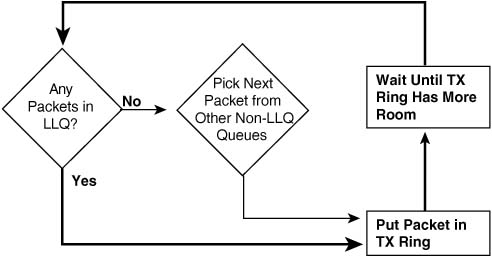
Note that like PQ, the LLQ scheduler always checks the low-latency queue first, and takes a packet from that queue. If there are no packets in the low-latency queue, the normal, scheduler logic applies to the other non-low-latency queue queues, giving them their guaranteed bandwidth.
For delay-sensitive traffic, the addition of a low-latency queue overcomes the one big negative of CBWFQ. In fact, with all the other queuing tools covered in this chapter so far, only PQ gave voice traffic the best quality. Of course, PQ had the negative side effect of almost destroying the performance of the lower-priority applications when the link was congested. With LLQ, you get the best of both worlds — low latency for the traffic in one queue, and guaranteed bandwidth for the traffic in other queues. Notice the thicker lines in Figure 5-21. If you follow these lines, you can see a path through the logic for LLQ in which only the low-latency queue gets any service. How can LLQ guarantee the other queues their respective bandwidths, with logic that never lets those queues get serviced? Well, the real answer is that Figure 5-21 is only part of the story. To prevent LLQ from having the same problem as PQ, where packets in the highest-priority queue could dominate and take all the available bandwidth, LLQ’s scheduler actually operates as shown in Figure 5-21.
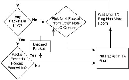
LLQ actually polices the PQ based on the configured bandwidth. By doing so, the packets in the queue that are forwarded still have very low latency, but LLQ also prevents the low-latency traffic from consuming more than its configured amount of bandwidth. By discarding excess traffic, LLQ can still provide bandwidth guarantees to the non-priority queues. The policing function works like policing as described in Chapter 6, but it is automatic in the low-latency queue — no additional policing configuration is required.
The policing function of LLQ takes care of protecting the other queues from the low-latency queue, but it does discard packets to accomplish that goal. Take a moment to reflect on the types of traffic that need to be classified into the low-latency queue. VoIP traffic, and in most cases, video traffic, need the low-latency, low-jitter performance of the low-latency queue. However, these are the same types of traffic that are most sensitive to dropped packets. So, although putting voice and interactive video into the low-latency queue may be good for queuing, discarding packets that exceed the configured rate for the queue would be harmful to those types of traffic. (Remember, interactive video needs low latency, but one-way video does not.)
The solution to the LLQ policing feature’s bad effect on VoIP and interactive video traffic lies outside the control of LLQ. The solution requires the engineer to use whatever means necessary to prevent more than the reserved bandwidth for a low-latency queue from getting introduced into the network. If the low-latency queue has 30 kbps reserved, for example, a single G.729 call will never cause the policer to discard a packet. If a second call occurs, the policer will discard packets, and both voice calls will sound bad. The solution requires some engineering, and some use of call admission control (CAC) tools, to prevent the low-latency queue from being oversubscribed.
LLQ configuration requires one more command in addition to the commands used for CBWFQ configuration. Instead of using the bandwidth command on a class, use the priority command. The syntax of the priority command is as foloows:
This class subcommand enables LLQ in this class, reserves bandwidth, and enables the policing function. You can also configure the burst for the policer with this command, and it defaults to 20 percent of the configured policing rate.
The priority command sets the guaranteed minimum bandwidth, which is also the maximum bandwidth! As mentioned earlier, LLQ polices the traffic in a class that uses the priority command and discards excess traffic. The burst parameter works just like bursts do for policing tools described in Chapter 6; refer to Chapter 6 for more details on the concepts behind policing.
In the following example, the final lab scenario used in the CBWFQ section is repeated, except that LLQ is also enabled. The class with VoIP traffic has reserved 58 kbps again, but this time using the priority command. With two VoIP calls, the voice sounds fine. The same familiar traffic flows are used — two VoIP calls, a NetMeeting video conference, HTTP with two different frames (important.jpg and not-so.jpg), and an FTP download. The configuration shows CB marking on ingress of R3’s E0/0, and CBWFQ on egress at R3’s S0/0. The criteria for each type of traffic is as follows:
![]() R3’s S0/0 is clocked at 128 kbps.
R3’s S0/0 is clocked at 128 kbps.
![]() VoIP payload is marked with DSCP EF, and placed in its own queue, using tail drop. This class gets 58 kbps.
VoIP payload is marked with DSCP EF, and placed in its own queue, using tail drop. This class gets 58 kbps.
![]() NetMeeting voice and video from Server1 to Client1 is marked with DSCP AF41, and placed in its own queue, using tail drop. This class gets 22 kbps.
NetMeeting voice and video from Server1 to Client1 is marked with DSCP AF41, and placed in its own queue, using tail drop. This class gets 22 kbps.
![]() Any HTTP traffic whose URL contains the string “important” anywhere in the URL is marked with AF21, and placed in its own queue. This class gets 20 kbps.
Any HTTP traffic whose URL contains the string “important” anywhere in the URL is marked with AF21, and placed in its own queue. This class gets 20 kbps.
![]() Any HTTP traffic whose URL contains the string “not-so” anywhere in the URL is marked with AF23, and placed in its own queue. This class gets 8 kbps.
Any HTTP traffic whose URL contains the string “not-so” anywhere in the URL is marked with AF23, and placed in its own queue. This class gets 8 kbps.
![]() All other traffic is marked with DSCP BE, and placed in its own queue, using WRED and WFQ. This class gets the remaining 20 kbps.
All other traffic is marked with DSCP BE, and placed in its own queue, using WRED and WFQ. This class gets the remaining 20 kbps.
Example 5-8 shows the configuration.
Example 5-8 LLQ for VoIP, CBWFQ for NetMeeting, HTTP “important,” HTTP “not-so” Important, and Everything Else
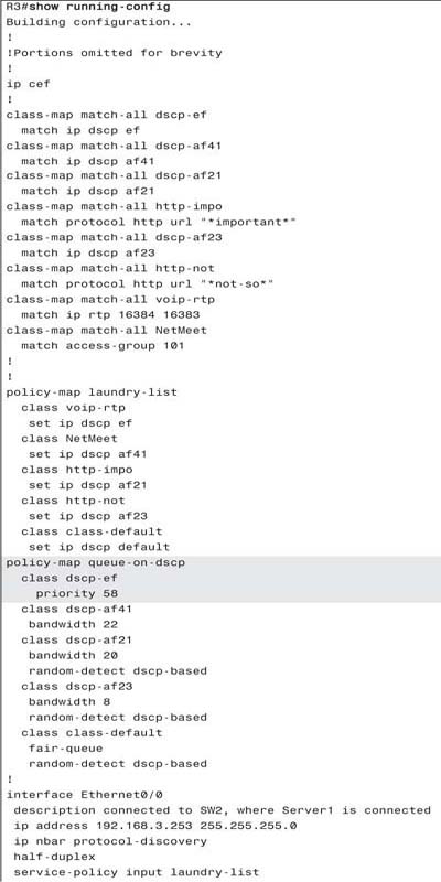

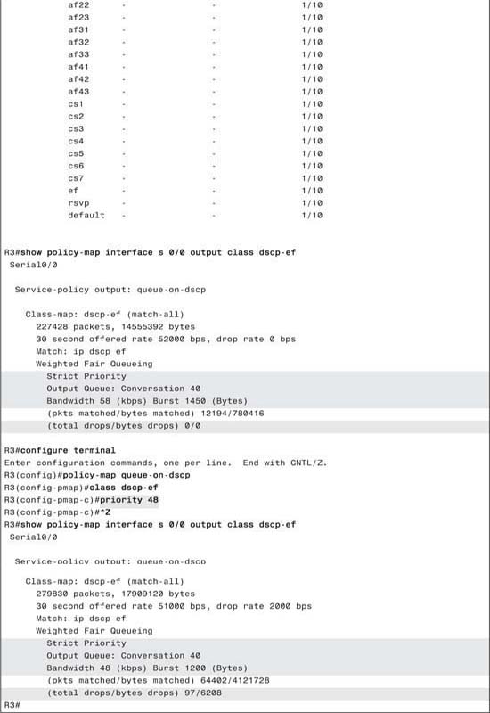
The only change to this configuration, when compared with the CBWFQ configuration in Example 5-8 is that in the dscp-ef class, inside policy-map queue-on-dscp, the priority command rather than the bandwidth command was used to reserve bandwidth. As seen in the output from the show policy-map command, IOS now performs strict-priority queuing on the traffic in class dscp-ef. Also note that the show policy-map output shows a burst value was defined (1450 bytes), which is used by the policing function of LLQ. The default burst size is equal to 200 milliseconds of traffic; 58000 bits/second * .2 seconds equals 11600 bits, or 1450 bytes.
Note also the drops experienced by the voice traffic as shown with the show policy-map interface s 0/0 output class dscp-ef command. The low-latency queue in this example has experienced zero drops, while providing the lowest possible latency for the voice traffic — which is exactly what you want for voice.
At the end of the example, the priority command was changed to reserve only 48 kbps. The two G.729 calls need about 52 kbps, and we know that LLQ polices. Notice that some packets have been dropped according to the final show policy command; this particular command was issued less than 10 seconds after changing the priority command to use only 48 kbps! In the time it took me to write this paragraph, the number of dropped packets had increased to 2000. Thus, the counters reinforce the fact that LLQ does indeed police the traffic. Therefore, you would need to use CAC mechanisms to prevent oversubscription of the low-latency queue.
Some Cisco documentation claims that you can only have one low-latency queue inside a single policy map. In other words, only one class can use the priority command, making it a low-latency queue. Other Cisco documentation claims that you can have more than one low-latency queue in a single policy map.
As it turns out, you can have multiple low-latency queues in a single policy map. Why would you need more than one low-latency queue in a policy map, and how would it work? Well, it’s actually pretty simple, now that you know how to configure LLQ.
First, imagine a policy map that has one low-latency queue configured with the priority 400 command. This queue needs 320 kbps for a single video conference call, plus three G.729 voice calls totaling about 80 kbps. If only the three voice calls and the single video-conference call occur, the LLQ configuration works fine, the policer does not drop any packets, and the voice and video packets are processed as FIFO within that LLQ class. As always, packets in the low- latency queue get serviced ahead of packets in the other non-LLQ classes.
Compare that configuration to a policy map with two low-latency queues defined — one for voice with a priority 80 command, and another for video conferencing with priority 320 configured. What’s really different about this than the first configuration? The policing, but not the queuing.
With multiple low-latency queues, each class is policed at the configured rate. For instance, with all voice calls going into the class with priority 80, three G.729 calls are supported, but not more than that. With video-conferencing traffic going into the class with priority 320, only that single video call is supported.
The fact that the different types of traffic are policed separately in the second example provides the motivation to use multiple low-latency queues. Suppose that a fourth voice call were made, and the CAC tools in place did not prevent the call, meaning that more than 80 kbps of voice traffic was being sent. With a single low-latency queue, both video and some voice packets would be discarded due to policing, because the cumulative rate for all traffic would exceed 400 kbps. The policer would have no way to decide to discard just the extra voice, but not video, because the policer acts on all traffic in the class. However, with the two low-latency queues configuration, only the voice calls would lose packets due to policing, and the video conference would not have any packets dropped by the policer.
In effect, with multiple low-latency queues, you get more granularity in what you police. In fact, the most typical reason to use multiple low-latency queues is to support voice in one queue, and video in another.
Queuing does not differ when comparing using a single low-latency queue with multiple low-latency queues in a single policy map. IOS always takes packets from the low-latency queues first, as compared with the non-low-latency queues (those with a bandwidth command), just like before. However, IOS does not reorder packets between the various low-latency queues inside the policy map. In other words, IOS treats all traffic in all the low-latency queues with FIFO logic.
In short, using multiple low-latency queues in one policy map does enable you to police traffic more granularly, but it does not reorder packets among the various low-latency queues.
When planning an LLQ configuration, you might frequently think of the LLQ traffic as needing an explicit amount of bandwidth. For instance, you plan for two G.729 calls, so you reserve 56 kbps for the call with the priority 56 class subcommand. In that case, you need a specific amount of bandwidth, not a percentage of the interface bandwidth.
Alternatively, if the interface had a bandwidth 256 command configured under it, you could have chosen to configure the priority percent 22 command, which would also reserve 56 kbps. However, if you ever increased the speed of the link, and updated the interface to use bandwidth 384, then the LLQ would end up with more bandwidth—22 percent of 384 kbps, or 84 bbps—but you might have still just wanted to support two voice calls. As a result, LLQ priority commands oftentimes show the explicitly configured bandwidth. So, more often than not, LLQ configurations define an explicit amount of link bandwidth, rather than a percentage.
Conversely, when reserving bandwidth for data, engineers often simply want to distribute the bandwidth by percentage. Earlier in this chapter, you read that you could use either the bandwidth class subcommand to reserve an explicit amount of bandwidth (for instance, bandwidth 56), or a percentage of the bandwidth defined for the interface (for instance, bandwidth percent 25). You can use either style of command. Either way works, but for data applications, a percentage of the bandwidth tends to work well.
Cisco provides yet another option for allocated bandwidth inside a policy map—an option that is particularly useful in many LLQ configurations. The command is bandwidth remaining percent, and it is particularly useful when an engineer wants a policy map that meets the following general concepts:
1. One or more LLQ classes need to be included in the policy map.
2. Some bandwidth is allocated for the class-default queue (that’s not a choice by the engineer—IOS always does this.)
3. For all the rest of the bandwidth, it would be best to subdivide the bandwidth based on a percentage of the bandwidth that was not already allocated — in other words, subdivide the remaining bandwidth after meeting the first two bandwidth requirements.
In short, if the goal is to create an LLQ configuration, with some non-LLQ queues, and you want to subdivide the bandwidth amongst the non-LLQs based on percentages, the bandwidth remaining percent command does the job. Example 5-9 shows an example configuration, along with some discussion of the numbers following the example.
Example 5-9 Examples Using the bandwidth remaining percent Command
Building configuration...
! Portions omitted for brevity
policy-map remaining-2
class class1
priority 55
class class2
bandwidth remaining percent 25
class class3
bandwidth remaining percent 35
class class4
bandwidth remaining percent 40
!
! Output omitted for brevity
!
interface Serial0/1
bandwidth 256
service-policy output remaining-2
R3#show policy-map interface s0/1
Serial0/1
Service-policy output: remaining-2
Class-map: class1 (match-all)
0 packets, 0 bytes
5 minute offered rate 0 bps, drop rate 0 bps
Match: ip dscp af41
Queueing
Strict Priority
Output Queue: Conversation 72
Bandwidth 55 (kbps) Burst 1375 (Bytes)
(pkts matched/bytes matched) 0/0
(total drops/bytes drops) 0/0
Class-map: class2 (match-all)
0 packets, 0 bytes
5 minute offered rate 0 bps, drop rate 0 bps
Match: ip dscp af42
Queueing
Output Queue: Conversation 73
Bandwidth remaining 25 (%) Max Threshold 64 (packets)
(pkts matched/bytes matched) 0/0
Class-map: class3 (match-all)
0 packets, 0 bytes
5 minute offered rate 0 bps, drop rate 0 bps
Match: ip dscp af43
Queueing
Output Queue: Conversation 74
Bandwidth remaining 35 (%) Max Threshold 64 (packets)
(pkts matched/bytes matched) 0/0
(depth/total drops/no-buffer drops) 0/0/0
Class-map: class4 (match-all)
0 packets, 0 bytes
5 minute offered rate 0 bps, drop rate 0 bps
Match: ip dscp af31
Queueing
Output Queue: Conversation 75
Bandwidth remaining 40 (%) Max Threshold 64 (packets)
(pkts matched/bytes matched) 0/0
(depth/total drops/no-buffer drops) 0/0/0
Class-map: class-default (match-any)
0 packets, 0 bytes
5 minute offered rate 0 bps, drop rate 0 bps
Match: any
In this example, the policy map provides the following bandwidth to the queues:
![]() 55 kbps to the LLQ (explicitly defined)
55 kbps to the LLQ (explicitly defined)
![]() 64 kbps for the class-default queue (25 percent of interface bandwidth)
64 kbps for the class-default queue (25 percent of interface bandwidth)
![]() 34 kbps (25 percent of 137 kbps) to class 2
34 kbps (25 percent of 137 kbps) to class 2
![]() 48 kbps (35 percent of 137 kbps) to class 3
48 kbps (35 percent of 137 kbps) to class 3
![]() 55 kbps (40 percent of 137 kbps) to class 4
55 kbps (40 percent of 137 kbps) to class 4
Two items are subtracted from the configured interface bandwidth in order to find the remaining bandwidth. As a quick review, the max-reserved-bandwidth command can be used to define how much interface bandwidth can be assigned to CBWFQ and LLQ classes, with the remainder being reserved for the class-default queue. In this case, 75 percent of 256 kbps is available to the all the non-class-default queues (192 kbps), with the rest (64 kbps) for the class-default queue. While you could change the max-reserved-bandwidth command setting under the interface, it is not generally recommended.
In this case, the remaining bandwidth for the non-LLQ queues ends up at 137 kbps. The logic flows like this:
1. Find the interface bandwidth as set with the bandwidth interface subcommand—in this case 256 kbps.
2. Subtract the bandwidth reserved for the class-default queue—in this case 64 kbps.
3. Subtract all bandwidth defined in LLQs—in this case 55 kbps.
4. The remaining amount of bandwidth is the bandwidth that is subdivided using the bandwidth remaining percent class subcommand, in this case, 137kbps.
Note The example showed how to use the bandwidth remaining percent class subcommand in conjunction with an LLQ configuration. However, you can also use it without LLQ, with a standard CBWFQ configuration. In that case, only the class-default bandwidth is subtracted from the interface bandwidth, with the remaining bandwidth being allocated using the bandwidth remaining percent command.
WFQ, CBWFQ, and LLQ each have an important role to play with QoS implementations in Cisco routers. WFQ works well as a default queuing mechanism when there are no low-latency requirements due to its very simple configuration and fair treatment of typically more important low volume flows. When an engineer takes the time to figure out what types of traffic need particular levels of service, CBWFQ provides bandwidth reservation with each class. When those types of traffic include classes with low latency and low jitter requirements, LLQ allows bandwidth reservation, priority service, with protection for the lower priority queues. Table 5-11 lists a few of the more important points about these queuing tools, with comments about their support of each point.

The “Foundation Summary” is a collection of tables and figures that provide a convenient review of many key concepts in this chapter. For those of you already comfortable with the topics in this chapter, this summary could help you recall a few details. For those of you who just read this chapter, this review should help solidify some key facts. For any of you doing your final preparation before the exam, these tables and figures are a convenient way to review the day before the exam.
The following list summarizes the key points about TX Rings and TX Queues in relation to their effect on queuing:
![]() The TX Queue/TX Ring always performs FIFO scheduling, and cannot be changed.
The TX Queue/TX Ring always performs FIFO scheduling, and cannot be changed.
![]() The TX Queue/TX Ring uses a single queue, per interface.
The TX Queue/TX Ring uses a single queue, per interface.
![]() IOS shortens the interface TX Queue/TX Ring automatically when an output queuing method is configured
IOS shortens the interface TX Queue/TX Ring automatically when an output queuing method is configured
![]() You can configure the TX Ring/TX Queue length to a different value.
You can configure the TX Ring/TX Queue length to a different value.
Figure 5-22 shows how Hardware Queues affect queuing. With queuing configured with two queues, seven packets arrive, numbered in the order in which they arrive. The output queuing configuration specifies that the first two packets (1 and 2) should be placed into Queue 2, and the next four packets (numbered 3 through 6) should be placed into Queue 1.
Figure 5-22 Two Output Queues, with Scheduler Always Servicing Queue 1 Rather Than Queue 2 When Packets Are in Queue 1

To delay the traffic, traffic shaping places the packets into the queue associated with the subinterface or DLCI and drains the traffic from the shaping queue at the shaped rate. Figure 5-23 shows the structure of the queues on a subinterface, interface, and the TX Queue, when shaping is enabled.
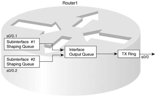
Flow-Based WFQ, or simply WFQ, classifies traffic into flows. Flows are identified by at least five items in an IP packet.
![]() Source IP address
Source IP address
![]() Destination IP address
Destination IP address
![]() Transport layer protocol (TCP or UDP) as defined by the IP Protocol header field
Transport layer protocol (TCP or UDP) as defined by the IP Protocol header field
![]() TCP or UDP source port
TCP or UDP source port
![]() TCP or UDP destination port
TCP or UDP destination port
![]() IP Precedence
IP Precedence
WFQ calculates the sequence number (SN) (also called Finish Time (FT)) before adding a packet to its associated queue. The formula for calculating the SN for a packet is as follows:
![]()
Table 5-12 lists the weight values used by WFQ as of 12.0(5)T/12.1.

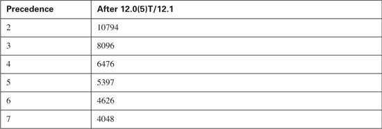
WFQ discards some packet when a queue’s congestive discard threshold (CDT) has been reached. To appreciate how the CDT is used, examine Figure 5-24.
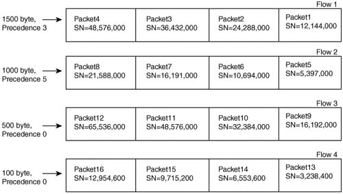
Table 5-13 summarizes some of the key features of WFQ.


Table 5-14 summarizes some of the key features of CBWFQ.

To prevent LLQ from having the same problem as PQ, where packets in the highest-priority queue could dominate, LLQ’s scheduler actually works as shown in Figure 5-25.

Table 5-15 lists a few of the more important points about these queuing tools, with comments about their support of each point.

This book attempts to cover the breadth and depth of QoS as covered on the QoS exam (642-642). However, you may want to read more about topics in this chapter, or other classification and marking topics.
For more on the topics in this chapter:
![]() Cisco IOS 12.3 QOS Configuration Guide (http://www.cisco.com/univercd/cc/td/doc/product/software/ios123/123cgcr/qos_vcg.htm)
Cisco IOS 12.3 QOS Configuration Guide (http://www.cisco.com/univercd/cc/td/doc/product/software/ios123/123cgcr/qos_vcg.htm)
For more on other Classification and Marking topics:
![]() Appendix B, “Additional QoS Reference Materials” (found on the book’s accompanying CD-ROM):
Appendix B, “Additional QoS Reference Materials” (found on the book’s accompanying CD-ROM):
— Priority Queuing (PQ)
— Custom Queuing (CQ)
— Modified Deficit Round Robin (MDRR)
For design related guidance:
![]() Cisco’s document “Cisco AVVID Network Infrastructure Enterprise Quality of Service Design” document at http://cisco.com/application/pdf/en/us/guest/netsol/ns17/c649/ccmigration_09186a00800d67ed.pdf
Cisco’s document “Cisco AVVID Network Infrastructure Enterprise Quality of Service Design” document at http://cisco.com/application/pdf/en/us/guest/netsol/ns17/c649/ccmigration_09186a00800d67ed.pdf
As mentioned in the Introduction, you have two choices for review questions. The questions that follow next give you a more difficult challenge than the exam itself by using an open-ended question format. By reviewing now with this more difficult question format, you can exercise your memory better, and prove your conceptual and factual knowledge of this chapter. You can find the answers to these questions in Appendix A.
The second option for practice questions is to use the CD included with this book. It includes a testing engine and more than 200 multiple-choice questions. You should use this CD nearer to the end of your preparation, for practice with the actual exam format.
|
1. |
Describe the benefits of having a single FIFO output queue. |
|
2. |
Explain the effects of changing a single FIFO queue’s length to twice its original value. Include comments about how the change affects bandwidth, delay, jitter, and loss. |
|
3. |
Explain the purpose of a TX Ring and TX Queue in a Cisco router. |
|
4. |
Explain how a long TX Ring might affect the behavior of a queuing tool. |
|
5. |
Describe the command output that identifies the length of the TX Ring or TX Queue, and whether the length was automatically lowered by IOS. |
|
6. |
Explain under what circumstances the TX Ring, interface output queues, and subinterface output queues both fill and drain, and to where they drain. |
|
7. |
Assume a queuing tool has been enabled on interface S0/0. Describe the circumstances under which the queuing tool would actually be used. |
|
8. |
Explain the circumstances under which it would be useful to enable a queuing tool on a subinterface. |
|
9. |
Describe the process and end result of the scheduling feature of Priority Queuing. |
|
10. |
Describe the process and end result of the scheduling feature of Custom Queuing. |
|
11. |
Describe how the Modified Deficit Round-Robin scheduler works, and specifically why the word “deficit” refers to part of the scheduler logic. |
|
12. |
WFQ classifies packets based on their flow. Other than a typical flow from an end user device, identify the other two types of flows recognized by WFQ. |
|
13. |
Characterize the effect the WFQ scheduler has on different types of flows. |
|
14. |
Describe the WFQ scheduler process. Include at least the concept behind any formulas, if not the specific formula. |
|
15. |
You previously disabled WFQ on interface S0/0. List the minimum number of commands required to enable WFQ on S0/0. |
|
16. |
What commands list statistical information about the performance of WFQ? |
|
17. |
Define what comprises a flow in relation to WFQ. |
|
18. |
You just bought and installed a new 3600 series router. Before adding any configuration to the router, you go ahead and plug in the new T1 Frame Relay access link to interface S0/0. List the minimum number of commands required to enable WFQ on S0/0. |
|
19. |
Describe the CBWFQ scheduler process, both inside a single queue and among all queues. |
|
20. |
Describe how LLQ allows for low latency while still giving good service to other queues. |
|
21. |
Compare and contrast the CBWFQ command that configures the guaranteed bandwidth for a class with the command that enables LLQ for a class. |
|
22. |
Describe the CBWFQ classification options. List at least five fields that can be matched without using an ACL. |
|
23. |
Name the two CBWFQ global configuration commands that define classification options, and then the per-hop behaviors, respectively. Also list the command that enables CBWFQ on an interface. |
|
24. |
Examine the following configuration (Example 5-10). Which of the five policy maps would certainly enable LLQ for voice payload traffic, based only of the information in the configuration? |
Example 5-10 Exhibit for CBWFQ Configuration Questions
class-map match-all class1
match ip rtp 16384 16383
class-map match-all class2
match access-group 101
class-map match-all class3
match ip rtp 16384 32767
class-map match-all class4
match ip dscp ef
match access-group 102
!
policy-map pmap1
class class1
priority 60
policy-map pmap2
class class2
priority 60
policy-map pmap3
class class3
priority 60
policy-map pmap4
class class4
priority 60
policy-map pmap5
class class5
priority 60
!
interface Serial0/0
service-policy output ?????
!
access-list 101 permit udp any gt 16383 any gt 16383
access-list 102 permit udp any range 16383 32767 any range 16383 32767
!
|
25. |
Using the same exhibit as in the preceding example, describe what must also be true for pmap4 to queue voice payload traffic successfully, and only voice payload traffic, in a low-latency queue. |
|
26. |
Which of the following queuing tools can always service a particular queue first, even when other queues have packets waiting? First-In, First-Out Queuing (FIFO); Priority Queuing (PQ); Custom Queuing (CQ); Weighted Fair Queuing (WFQ); Class-Based WFQ (CBWFQ); Low Latency Queuing (LLQ). |
|
27. |
Which of the following queuing tools allows for a percentage bandwidth to be assigned to each queue? First-In, First-Out Queuing (FIFO); Priority Queuing (PQ); Custom Queuing (CQ); Weighted Fair Queuing (WFQ); Class-Based WFQ (CBWFQ); Low Latency Queuing (LLQ). |
|
28. |
Which queuing tools could be configured to provide the lowest possible latency for voice traffic? Of these, which does Cisco recommend as the best option for voice queuing today? |
|
29. |
Which of the following queuing tools can use flow-based classification? First-In, First-Out Queuing (FIFO); Priority Queuing (PQ); Custom Queuing (CQ); Weighted Fair Queuing (WFQ); Class-Based WFQ (CBWFQ); Low Latency Queuing (LLQ). |
|
30. |
Which of the following queuing tools uses the Modular QoS CLI? First-In, First-Out Queuing (FIFO); Priority Queuing (PQ); Custom Queuing (CQ); Weighted Fair Queuing (WFQ); Class-Based WFQ (CBWFQ); Low Latency Queuing (LLQ). |
|
31. |
Which of the following queuing tools allows for a value to be configured, which then results in a specific number of bytes being taken from each queue during a round-robin pass through the queues? First-In, First-Out Queuing (FIFO); Priority Queuing (PQ); Custom Queuing (CQ); Weighted Fair Queuing (WFQ); Class-Based WFQ (CBWFQ); Low Latency Queuing (LLQ). |
|
32. |
What model of Cisco router supports WFQ inside CBWFQ classes other than class-default? |
|
33. |
Give an explanation for the following comment: “WFQ can become too fair when it has a large number of active flows”? |
|
34. |
Imagine the following commands in Example 5-11 were typed in configuration mode, in order. Also assume that class maps class1, class2, and class3 have already been correctly defined. How much bandwidth will class class3 be assigned on interface S0/0? |
Example 5-11 Exhibit for CBWFQ Configuration Questions
policy-map pmap1
class class1
priority 60
class class2
bandwidth percent 30
class class3
bandwidth percent 45
!
policy-map pmap2
class class1
priority percent 20
class class2
bandwidth remaining percent 30
class class3
bandwidth remaining percent 70
!
policy-map pmap3
class class1
priority percent 20
class class2
bandwidth 30
class class3
bandwidth percent 30
!
interface Serial0/0
service-policy output pmap1
!
|
35. |
In the same example, what could be done so that the service-policy output pmap1 command would be accepted under interface serial0/0—without changing the policy map? Assuming that was done, what actual bandwidth could be assigned to class3? |
|
36. |
In the same example, how much bandwidth would class1 be assigned on interface serial 0/1? |
|
37. |
In the same example, how much bandwidth would class2 and class3 be assigned on interface serial 0/1? |
|
38. |
In the same example, how much bandwidth would class2 and class3 be assigned on interface serial 0/2? |