Appendix B. Additional QoS Reference Materials
A few years ago, Cisco introduced a couple of different QoS courses, along with a couple of different QoS exams, called DQOS and QOS. The two exams had about 60 percent overlap with each other, but the DQOS exam and course focused more on Enterprises and VoIP, whereas the QoS exam and course focused more on QoS issues in Service Provider networks.
To support the exams, Cisco Press also came out with the first edition of this book, which focused on the DQOS exam, but included coverage of most of the topics on the QoS exam that weren’t also on the DQOS exam.
Later, mainly early in 2004, Cisco changed to have a single QoS course and exam (642-642). The two courses essentially merged, with some topics being removed, and with several new topics being added. Also, topics that were in the older courses were updated based on the Cisco IOS Software Release 12.2T/12.3 revisions.
Personally, I think Cisco definitely had the right idea with the update to the new QoS course and exam. The course and exam focus on the most appropriate QoS tools today, at least when running the latest IOS releases. So, for people just looking to build skills for today’s new networks, the scope of the topics on the exam is well chosen.
However, for a couple of reasons, we decided to include several topics from the First Edition of this book in an appendix. The first reason is that a lot of CCIE Route/Switch and CCIE Voice candidates had been looking for a good QoS book to use to study for their labs, and the materials in the First Edition were popular with those folks.
Another justification for the inclusion of this appendix is that a few topics are good background for people deploying QoS in real networks. According to Cisco’s website, Cisco IOS Software Release 12.2 reached General Deployment (GD) status in February of 2004. Some customers tend to wait on GD status before migrating to a new IOS release. So, for partner engineers, some customers simply won’t be able to take advantage of some of the newer QoS features. So, this appendix might be a nice reference.
Finally, we wanted to keep the FRTS configuration section around. The current QoS exam (642-642) does not cover Frame Relay Traffic Shaping (FRTS) as an end to itself, but it does cover FRF.12 Fragmentation[md]which requires FRTS. This appendix provides a little more background on FRTS.
Finally, a word of disclaimer. The topics in appendix were taken from the first edition of this book, which was based on features available with Cisco IOS Software Release 12.1(5)T. for the most part. We did not update these topics based on later IOS releases. We offer this appendix for those people who might find it useful, but please be aware that it is outdated compared to the later IOS releases. In fact, there may be a few cases where this appendix contradicts the core chapters in the book because of those changes; when in doubt, trust the core chapters, and not this appendix, in regards to the QoS exam.
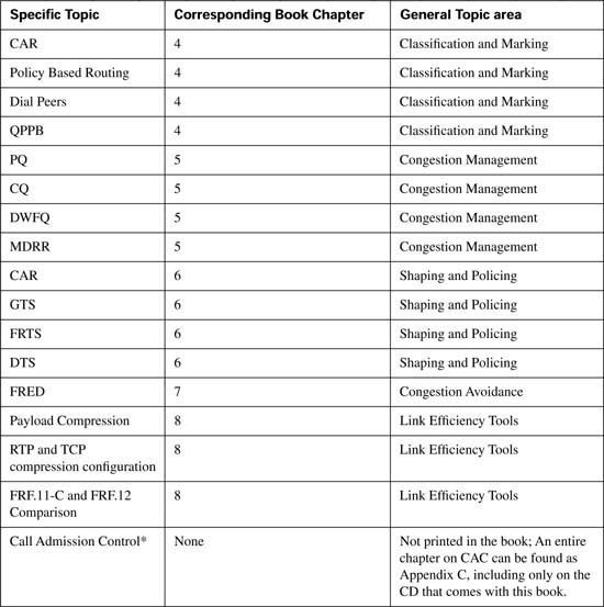
The topics in this chapter are organized in the same general order as the topics in the core of the book. However, keep in mind that the topics are essentially a collection of short topics. Table B-1 lists the topics in this chapter.
This section covers CAR (as a marking tool), Policy Based Routing (as a marking tool), Dial-peers, and QoS Policy Propagation with BGP.
CAR provides policing functions and marking. Chapter 5, “Traffic Policing and Shaping,” covers the policing details of CAR and CB policing. However, a quick review of policing before getting into CAR’s marking features will help you appreciate why CAR includes marking.
Policing, in its most basic form, discards traffic that exceeds a particular traffic contract. The contract has two components: a rate, stated either in bits per second or bytes per second; and a burst size, stated in either bits or bytes. The traffic conforms to the contract if it sends at the rate, or below, and it does not send a burst of traffic greater than the burst size. If the traffic exceeds the traffic rate over time, or exceeds the single burst size limit, the policing function drops the traffic in excess of the rate and the burst size. Therefore, the simplest form of policing has two rigid actions: either to forward packets or to drop them.
CAR’s marking function allows for additional policing action besides just forwarding or dropping a packet. Consider a typical case where policing is used, as in Figure B-1. ISP1 needs to police traffic to protect customers who conform to their contracts from congestion created by customers who do not conform. If the network is not congested, however, it might be nice to go ahead and forward the nonconforming customer traffic. Doing so doesn’t really cost the ISP anything, so long as the network is not congested. If the network is congested, however, ISP1 wants to discard the traffic that exceeds the contract before discarding traffic that is within its respective contract.

For instance, the conforming traffic can be marked with DSCP AF41, and the nonconforming traffic with DSCP Default. The congestion-avoidance QoS tools in ISP1 can be configured to aggressively discard all DSCP Default traffic at the first signs of congestion. So, when ISP1 experiences congestion, policing indirectly causes the excess traffic to be discarded; in periods of no congestion, ISP1 provides service beyond what the customer has paid for.
You can also use CAR to just mark the traffic. CAR classifies traffic based on a large number of fields in the packet header, including anything that can be matched with an IP ACL. Once matched, CAR can be configured to do one action for conforming traffic, and another for excess traffic. If the two actions (conform and exceed actions) are the same action, in effect, CAR has not policed, but rather has just marked packets in the same way.
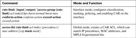
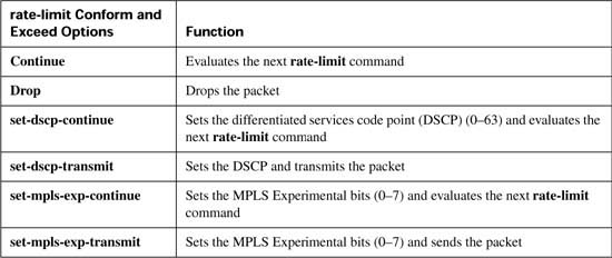
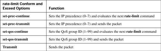
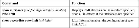
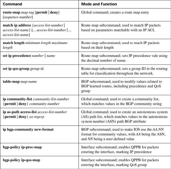
CAR configuration includes the classification, marking, and enabling features all in a single configuration command: the rate-limit interface subcommand. (CB marking, you may recall, separates classification, marking, and enabling on an interface into three separate commands.) Tables B-2, B-3, and B-4 list the pertinent CAR configuration and exec commands, respectively.
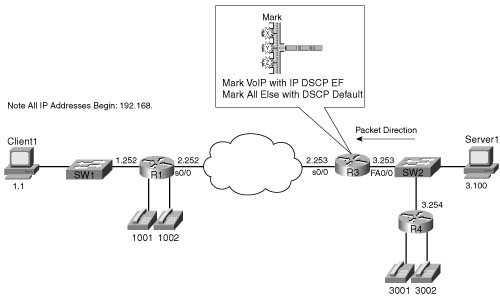
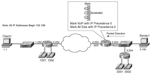
The first CAR marking example, shown in Example B-1, uses the following criteria for marking packets. In this example, R3 is marking packets that flow right to left in Figure B-2.
![]() All VoIP payload traffic is marked with DSCP EF.
All VoIP payload traffic is marked with DSCP EF.
![]() All other traffic is marked with DSCP Default.
All other traffic is marked with DSCP Default.
Example B-1 CAR Marking, VoIP as DSCP EF, Everything Else as BE
no ip cef
!
access-list 102 permit udp any range 16384 32768 any range 16384 32768
!
interface fastethernet 0/0
rate-limit input access-group 102 10000 20000 30000 conform-action
set-dscp-transmit 46 exceed-action set-dscp-transmit 46
rate-limit input 10000 20000 30000 conform-action set-dscp-transmit 0
exceed-action set-dscp-transmit 0
end
The configuration does not take nearly as many different commands as the CB marking example, because most of the interesting parameters are contained in the rate-limit commands. Cisco Express Forwarding (CEF) is disabled, just to make the point that although you can use CEF with CAR, it is not required. ACL 102 defines some classification parameters that CAR will use to match VoIP packets, looking at UDP ports between 16,384 and 32,767. The ACL logic matches all VoIP payload, but it will also match VoIP Real Time Control Protocol (RTCP) traffic, which uses the odd-numbered UDP ports in the same port range. Finally, two rate-limit commands under FA0/0 enable CAR, define policing limits, classification details, and marking details.
The first of the two rate-limit commands matches a subset of all traffic using classification, whereas the second rate-limit command just matches all traffic. CAR uses the information configured in these two commands sequentially; in other words, if a packet matches the first CAR statement’s classification details, the statement is matched, and its actions are followed. If not, CAR compares the next statement, and so on. In this example, the first CAR rate-limit command matches VoIP packets by referring to ACL 102, and the second statement, because it does not refer to an ACL, matches all packets.
Note CAR can actually match multiple statements on the same interface. Some CAR actions include the keyword continue, which means that even after the statement is matched, CAR should keep searching the statements for further matches. This allows CAR to nest statements, to perform features such as “police all traffic at 500 kbps, but police subsets at 250 kbps, 200 kbps, and 150 kbps.”
Now examine the first rate-limit command, rate-limit input access-group 102 10000 20000 30000 conform-action set-dscp-transmit 46 exceed-action set-dscp-transmit 46, in detail. The input keyword means that CAR examines traffic entering the interface. The access-group 102 command means that packets permitted by ACL 102 are considered to match this rate-limit command. The next three values represent the committed rate, the burst size, and the excess size, which make up the traffic contract. The conform-action keyword identifies that the next parameter defines the action applied to conforming traffic, and the exceed-action keyword identifies that the next parameter defines the action applied to traffic that exceeds the traffic contract. In this example, both the conform and exceed actions are identical: set-dscp-transmit 46, which marks the DSCP value to decimal 46, or DSCP EF. (The rate-limit command does not allow the use of DSCP names.)
In this example, the actual traffic contract does not matter, because the actions for conforming traffic and excess traffic are the same. The true goal of this example is just to use CAR to mark packets VoIP—not to actually police the traffic. Chapter 5 includes CAR examples with different conform and exceed actions. The three values represent the committed rate (bps), the committed burst size (bytes), and the committed burst plus the excess burst (bytes). The excess burst parameter essentially provides a larger burst during the first measurement interval after a period of inactivity. (Chapter 5 covers the details of these settings.)
The second rate-limit command, rate-limit input 10000 20000 30000 conform-action set-dscp-transmit 0 exceed-action set-dscp-transmit 0, matches all remaining traffic. The only way that CAR can classify packets is to refer to an IP ACL, or a CAR rate-limit ACL, from the rate-limit command. The second rate-limit command does not refer to an ACL with the access-group keyword, so by implication, the statement matches all packets. Both actions set the DSCP value to zero. Essentially, this example uses CAR to mark traffic with either DSCP 46 or 0 (decimal), without discarding any packets due to policing.
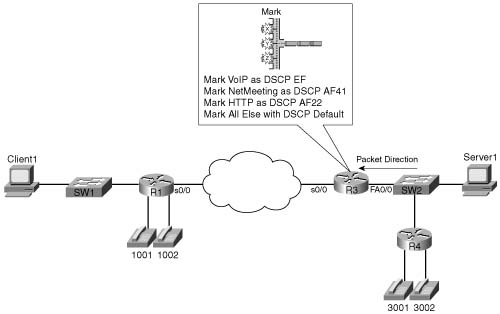
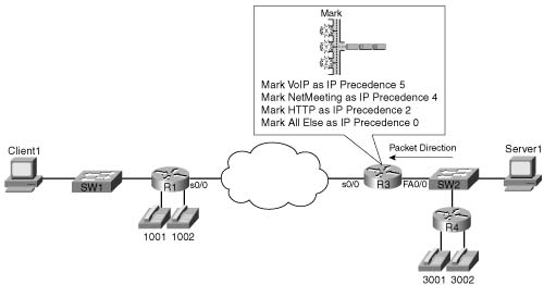
Because CAR cannot take advantage of NBAR, CAR cannot look at the URL for HTTP requests, as the CB marking example did. The slightly modified criteria for CAR marking in Example B-2 is as follows:
![]() VoIP payload is marked with DSCP EF.
VoIP payload is marked with DSCP EF.
![]() NetMeeting voice and video from Server1 to Client1 is marked with DSCP AF41.
NetMeeting voice and video from Server1 to Client1 is marked with DSCP AF41.
![]() Any HTTP traffic is marked with AF22.
Any HTTP traffic is marked with AF22.
![]() All other traffic is marked with DSCP Default.
All other traffic is marked with DSCP Default.
Figure B-3 shows the network in which the configuration is applied, and Example B-2 shows the configuration.
Example B-2 CAR Marking Sample 2: VoIP, NetMeeting Audio/Video, HTTP URLs, and Everything Else
no ip cef
!
access-list 110 permit udp any range 16384 32768 any range 16384 32768
!
access-list 111 permit udp host 192.168.1.100 gt 16383 192.168.3.0 0.0.0.255 gt 16383
!
access-list 112 permit tcp any eq www any
access-list 112 permit tcp any any eq www
!
!
rate-limit input access-group 111 8000 20000 30000 conform-action
set-dscp-transmit 34 exceed-action set-dscp-transmit 34
rate-limit input access-group 110 8000 20000 30000 conform-action
set-dscp-transmit 46 exceed-action set-dscp-transmit 46
rate-limit input access-group 112 8000 20000 30000 conform-action
set-dscp-transmit 20 exceed-action set-dscp-transmit 20
rate-limit input 8000 20000 30000 conform-action set-dscp-transmit 0
exceed-action set-dscp-transmit 0
end
R3#show interface fastethernet 0/0 rate-limit
Fastethernet0/0 connected to SW2, where Server1 is connected
Input
matches: access-group 111
params: 8000 bps, 20000 limit, 30000 extended limit
conformed 1346 packets, 341169 bytes; action: set-dscp-transmit 34
exceeded 2683 packets, 582251 bytes; action: set-dscp-transmit 34
last packet: 56ms ago, current burst: 29952 bytes
last cleared 00:07:11 ago, conformed 6000 bps, exceeded 10000 bps
matches: access-group 110
params: 8000 bps, 20000 limit, 30000 extended limit
conformed 6118 packets, 452856 bytes; action: set-dscp-transmit 46
exceeded 34223 packets, 2552218 bytes; action: set-dscp-transmit 46
last packet: 12ms ago, current burst: 29989 bytes
last cleared 00:07:11 ago, conformed 8000 bps, exceeded 47000 bps
matches: access-group 112
params: 8000 bps, 20000 limit, 30000 extended limit
conformed 677 packets, 169168 bytes; action: set-dscp-transmit 20
exceeded 3631 packets, 5084258 bytes; action: set-dscp-transmit 20
last packet: 8ms ago, current burst: 29638 bytes
last cleared 00:07:12 ago, conformed 3000 bps, exceeded 94000 bps
matches: all traffic
params: 8000 bps, 20000 limit, 30000 extended limit
conformed 671 packets, 279572 bytes; action: set-dscp-transmit 0
The show interface Fastethernet 0/0 rate-limit command lists the pertinent statistical information about CAR’s performance. The output has one stanza correlating to each rate-limit command on the interface, as highlighted in the example. Under each stanza, the number of packets and bytes that conformed, and the number of packets and bytes that exceeded the traffic contract, are listed. Because this CAR configuration was intended only for marking traffic, the number of packets and bytes in each category does not matter; Chapter 6, “Traffic Policing and Shaping,” takes a closer look at the two values. For comparison purposes, however, consider the bps rates of the combined conformed and exceeded values. For instance, the second rate-limit command referenced ACL 110, which matched the two VoIP calls between R1 and R4. These two values total 55 kbps, which is the amount of traffic expected from a pair of G.729a calls over an Ethernet network.
CAR is another tool that examines packet header information to classify and mark packets. CAR provides fewer options for classification and marking than does CB marking, but CAR is considered to be DiffServ compliant because it can classify DSCP using an ACL and mark the DSCP field directly. CAR, along with CB marking and PBR, makes classification decisions based on the contents of packet headers and marks QoS fields based on those classifications. Dial peers provide very different classification options, so fewer direct comparisons can be drawn.
Refer to Table B-3 for a complete list of classification and marking fields used by CAR.
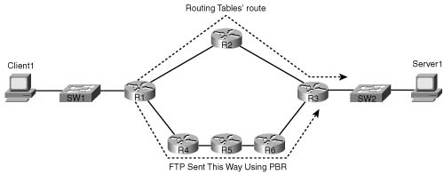
PBR enables you to route a packet based on other information, in addition to the destination IP address. In most cases, engineers are happy with the choices of routes made by the routing protocol, with routing occurring based on the destination IP address in each packet. For some specialized cases, however, an engineer may want some packets to take a different path. One path through the network may be more secure, for instance, so some packets could be directed through a longer, but more secure, path. Some packets that can tolerate high latency may be routed through a path that uses satellite links, saving bandwidth on the lower-latency terrestrial circuits for delay-sensitive traffic. Regardless of the reasons, PBR can classify packets and choose a different route. Figure B-4 shows a simple example, where FTP traffic is directed over the longer path in the network.
PBR supports packet marking and policy routing. As you learned in previous sections, CAR supports marking because CAR’s main feature, policing, benefits from having the marking feature available as well. Similarly, PBR includes a marking feature, because in some cases, PBR is used to pick a different route for QoS reasons—for instance, to affect the latency of a packet. So, PBR’s core function can benefit from marking a packet, so that the appropriate QoS action can be taken as the packet traverses the network. Just as with CAR, you can use PBR’s marking feature without actually using its core feature. In other words, you can use PBR just for classification and marking, without choosing a different route. The examples in this chapter focus only on PBR as a marking tool.
Unlike CB marking and CAR, PBR only processes packets entering an interface; you cannot enable it for packets exiting an interface. The reason PBR only processes incoming packets relates to its core function: policy routing. PBR needs to process packets before a routing decision has been made. Therefore, PBR processes packets entering an interface, preempting the normal routing logic based on destination IP address.
Finally, one other difference between PBR and the other classification and marking tools covered so far (CB marking and CAR) is that PBR can classify based on routing information, instead of totally relying on information in the frame or packet header. PBR can look up the entry in the routing table that matches a packet’s destination address, for instance, and then classify based on information about that route. For example, the metric associated with that route, the source of the routing information, or the next-hop interface associated with the route can be checked. In most cases, this routing information does not help you with differentiating between different types of traffic. An FTP server, an IP Phone, a video server, and some web servers may all be in the same subnet, for instance, but the routing information about that subnet could not help PBR distinguish between those different types of traffic. Therefore, typically the most useful classification feature of PBR, when used for marking, is just to refer to an IP ACL.
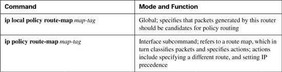
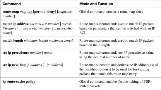
PBR configuration uses yet another totally different set of configuration commands as compared to CB marking and CAR. PBR does separate the classification, marking, and enabling features into different commands. Tables B-5 and B-6 list the pertinent PBR configuration and exec commands, respectively. Following the tables, two example PBR configurations are shown. The two examples use the same criteria as the two CAR samples.
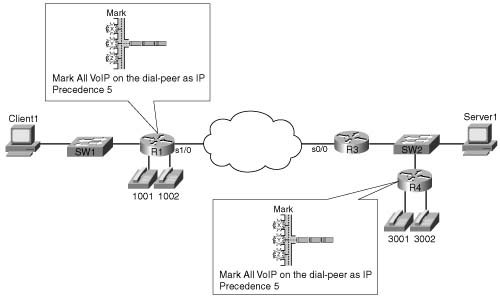
Example B-3 shows the first PBR marking example, which uses the same criteria as Example B-1 for CAR. In this example, R3 is marking packets that flow right to left in Figure B-5.
![]() All VoIP payload traffic is marked with IP precedence 5.
All VoIP payload traffic is marked with IP precedence 5.
![]() All other traffic is marked with IP precedence 0.
All other traffic is marked with IP precedence 0.
Figure B-5 PBR Marking Sample 1: VoIP Marked with IP Precedence 5, Everything Else Marked IP Precedence 0
PBR uses route-map commands, along with match and set route-map subcommands, to classify and mark the packets. This configuration uses a route map named voip-routemap, which includes two clauses. The first clause, clause 10, uses a match command that refers to VoIP-ACL, which is a named IP ACL. VoIP-ACL matches UDP port numbers between 16,384 and 32,767, which matches all VoIP traffic. If the ACL permits a packet, the route map’s first clause acts on the set command, which specifies that IP precedence should be set to 5.
The second route map clause, clause 20, matches the rest of the traffic. The route map could have referred to another IP ACL to match all packets; however, by not specifying a match statement in clause 20, all packets will match this clause by default. By not having to refer to another IP ACL to match all packets, less processing overhead is required. The set command then specifies to set precedence to zero.
The ip policy route-map voip-routemap command enables PBR on interface FA0/0 for incoming packets. Notice that the direction, input or output, is not specified, because PBR can only process incoming packets.
The last PBR-specific command is ip route-cache policy. IOS process-switches PBR traffic by default; to use fast switching on PBR traffic, use the ip route-cache policy command.
The second PBR configuration (Example B-4) includes classification options identical to CAR example 2 (see Example B-2). A major difference between PBR and CAR is that PBR cannot set the DSCP field, so it sets the IP Precedence field instead. The slightly modified criteria, as compared with CAR example 2, for PBR example 2 is as follows:
![]() VoIP payload is marked with precedence 5.
VoIP payload is marked with precedence 5.
![]() NetMeeting voice and video from Server1 to Client1 is marked with precedence 4.
NetMeeting voice and video from Server1 to Client1 is marked with precedence 4.
![]() Any HTTP traffic is marked with precedence 2.
Any HTTP traffic is marked with precedence 2.
![]() All other traffic is marked with precedence 0.
All other traffic is marked with precedence 0.
Figure B-6 shows the network in which the configuration is applied, and Example B-4 shows the configuration.
Example B-4 PBR Marking Sample 2: VoIP, NetMeeting Audio/Video, HTTP URLs, and Everything Else
ip route-cache policy
!
ip access-list extended VoIP-ACL
permit udp any range 16384 32768 any range 16384 32768
!
ip access-list extended NetMeet-ACL
permit udp host 192.168.1.100 range 16384 32768 192.168.3.0 0.0.0.255 range 16384 32768
!
!
ip access-list extended http-acl
permit tcp any eq www any
permit tcp any any eq www
!
interface fastethernet 0/0
ip policy route-map voip-routemap
!
route-map voip-routemap permit 10
match ip-address NetMeet-ACL
set ip precedence 4
!
route-map voip-routemap permit 20
match ip-address VoIP-ACL
set ip precedence 5
!
route-map voip-routemap permit 30
match ip-address http-acl
set ip precedence 2
!
route-map voip-routemap permit 40
set ip precedence 0
!
end
R3#sh ip policy
Interface Route map
Fastethernet0/0 voip-routemap
R3#show route-map
route-map voip-routemap, permit, sequence 10
Match clauses:
ip address (access-lists): NetMeet-ACL
Set clauses:
ip precedence flash-override
Policy routing matches: 3 packets, 222 bytes
route-map voip-routemap, permit, sequence 20
Match clauses:
Set clauses:
ip precedence critical
Policy routing matches: 14501 packets, 1080266 bytes
route-map voip-routemap, permit, sequence 30
Match clauses:
ip address (access-lists): http-acl
Set clauses:
ip precedence immediate
Policy routing matches: 834 packets, 1007171 bytes
route-map voip-routemap, permit, sequence 40
Match clauses:
Set clauses:
ip precedence routine
Policy routing matches: 8132 packets, 11263313 bytes
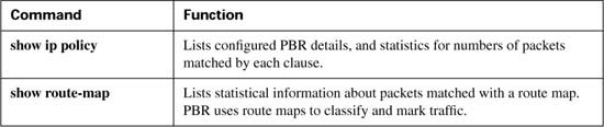
The output of the show ip policy command lists only sparse information. The show route-map command enables you to view statistical information about what PBR has performed. This command lists statistics for any activities performed by a route map, including when one is used for PBR. Notice that the four sets of classification criteria seen in the configuration are listed in the highlighted portions of the show route-map output, as are packet and byte counters.
PBR provides another classification and marking tool that examines packet header information to classify and mark packets. PBR is unique compared to the other tools in that it can classify based on information about the route that would be used for forwarding a packet. However, PBR has fewer options for matching header fields for classification as compared with the other tools.
PBR can mark IP precedence, QoS group, as well as the ToS bits. Refer to Table B-5, in the summary for this chapter, for a complete list of classification and marking fields used by PBR.
PBR provides a strong option for classification and marking in two cases. For applications when marking based on routing information is useful, PBR can look at details about the route used for each packet, and make marking choices. The other application for PBR marking is when policy routing is already needed, and marking needs to be done at the same time. For more general cases of classification and marking, CB marking or CAR is recommended.
IOS voice gateways provide many services to connect the packetized, VoIP network to nonpacketized, traditional voice services, including analog and digital trunks. IOS gateways perform many tasks, but one of the most important tasks is to convert from packetized voice to nonpacketized voice, and vice versa. In other words, voice traffic entering a router on an analog or digital trunk is not carried inside an IP packet, but the IOS gateway converts the incoming voice to a digital signal (analog trunks only) and adds the appropriate IP, UDP, and RTP headers around the digital voice (both analog and digital trunks). Conversely, when a VoIP packet arrives, and the voice needs to be sent out a trunk, the IOS gateway removes the packet headers, converts the voice to analog (analog trunks only), and sends the traffic out the trunk.
Although this book does not attempt to explain voice configuration and concepts to much depth, some appreciation for IOS gateway configuration is required for some of the functions covered in this book. In particular, Chapter 8, “Call Admission Control and QoS Signaling,” which covers Voice call admission control (CAC), requires a little deeper examination of voice. To understand classification and marking using dial peers, however, only a cursory knowledge of voice configuration is required. Consider Figure B-7, for instance, which shows two analog IOS voice gateways, R1 and R4, along with Examples B-5 and B-6, which show the pertinent configuration on R1 and R4.
Example B-5 R1 Voice Gateway Configuration
hostname R1
!
int fastethernet 0/0
ip address 192.168.1.251 255.255.255.0
!
dial-peer voice 3001 voip
destination-pattern 3001
session target ipv4:192.168.3.254
!
dial-peer voice 3002 voip
destination-pattern 3002
session target ipv4:192.168.3.254
!
dial-peer voice 1001 pots
destination-pattern 1001
port 3/0
!
dial-peer voice 1002 pots
destination-pattern 1002
port 3/1
Example B-6 R4 Voice Gateway Configuration
hostname R4
!
int fastethernet 0/0
ip address 192.168.3.254 255.255.255.0
!
dial-peer voice 1001 voip
destination-pattern 1001
session target ipv4:192.168.1.251
!
dial-peer voice 1002 voip
destination-pattern 1002
session target ipv4:192.168.1.251
!
dial-peer voice 3001 pots
destination-pattern 3001
port 3/0
!
dial-peer voice 3002 pots
destination-pattern 3002
port 3/1
The highlighted portions of the examples focus on the configuration for the physical voice ports on R1, and the VoIP configuration on R4. Both R1 and R4 use dial-peer commands to define their local analog voice trunks and to define peers to which VoIP calls can be made. In Example B-5, for instance, the highlighted portion of the configuration shows R1’s configuration of the two local analog lines. The two highlighted dial-peer statements use the keyword pots, which stands for plain-old telephone service. The pots keyword implies that the ports associated with this dial peer are traditional analog or digital telephony ports. The physical analog ports are correlated to each dial peer with the port command; in each of these configurations, a two-port FXS card sits inside slot 3 of a 1760-V router. Finally, on R1, the phone number, or dial pattern, associated with each of the analog ports is configured. With just the highlighted configuration in R1, voice calls could be placed between the two extensions (x1001 and x1002).
To place calls to extensions 1001 and 1002 from R4, the dial-peer commands highlighted in Example B-6 are required. These two dial-peer commands use a voip keyword, which means this dial peer configures information about an entity to which VoIP calls can be placed. The phone number, or dial pattern, is defined with the destination-pattern command again—notice that extensions 1001 and 1002 are again configured. Finally, because these two dial peers configure details about a VoIP call, a local physical port is not referenced. Instead, the session- target ipv4:192.168.1.251 command implies that when these phone numbers are called, to establish a VoIP call, using the IP version 4 IP address shown.
Similarly, R4 defines the local phone numbers and ports for the locally connected phones, and R1 defines VoIP dial peers referring to R4’s phones, so that calls can be initiated from R1.
Dial-peer classification and marking, when you know how to configure the basic dial-peer parameters, is easy. POTS dial peers refer to analog or digital trunks, over which no IP packet is in use—so there is nothing to mark. On VoIP dial peers, the dial peer refers to the IP address of another gateway to which a call is placed. So, by placing the ip precedence 5 dial-peer subcommand under each voip dial-peer, the packets generated for calls matching each dial peer will be marked with IP precedence 5. Example B-7 lists the R4 configuration, with these changes made; the equivalent changes would be made to R1 as well.
Example B-7 R4 Voice Gateway Configuration
hostname R4
!
interface fastethernet 0/0
ip address 192.168.3.254 255.255.255.0
!
dial-peer voice 1001 voip
session target ipv4:192.168.1.251
ip precedence 5
no vad
!
dial-peer voice 1002 voip
destination-pattern 1002
session target ipv4:192.168.1.251
ip precedence 5
no vad
!
dial-peer voice 3001 pots
destination-pattern 3001
port 3/0
!
dial-peer voice 3002 pots
destination-pattern 3002
port 3/1
In the example, the highlighted text shows the ip precedence 5 commands under each voip dial-peer. Packets created for VoIP calls for the configured dial patterns of 1001 and 1002 will be marked with IP precedence 5. The identical commands would be added to R1’s configuration on the VoIP dial peers to achieve the same effect.
Beginning in IOS Releases 12.2(2)XB and 12.2(2)T the ip precedence command has been replaced with the ip qos dscp command. This allows the dial peer to set the IP precedence or the DSCP value for VoIP payload and signaling traffic. Also keep in mind that the current DQOS exam, at the time this book was published, was based on IOS 12.1(5)T—so this command would not be on the current exam. Check the URLs listed in the Introduction for any possible changes.
The command uses the following syntax:
Table B-7 outlines the meaning of the parameters of the command.
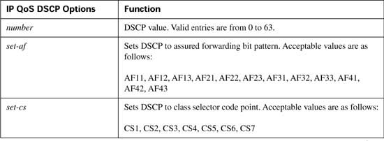
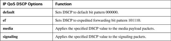
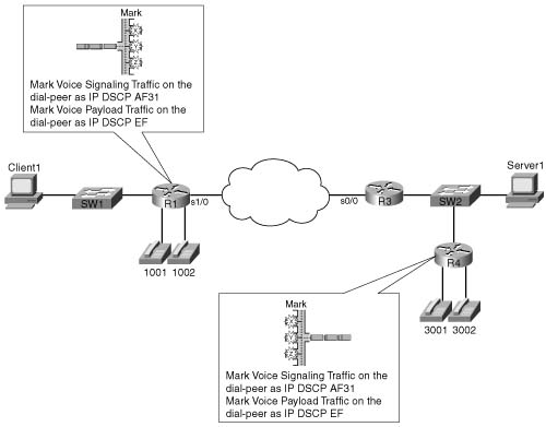
The ip qos dscp command enables you to have much more granular control of how a VoIP packet is marked than the ip precedence command, while providing a method to preserve backward compatibility. Examples B-8 and B-9 show how R1 and R4 can be configured to use the ip qos dscp command to mark voice payload traffic with a DSCP value of EF and voice signaling traffic with a DSCP value of AF31. Figure B-8 shows the now-familiar network, with the new criteria listed.
Example B-8 R1 IP QoS DSCP Dial-Peer Configuration
!
int fastethernet 0/0
ip address 192.168.1.251 255.255.255.0
!
dial-peer voice 3001 voip
destination-pattern 3001
ip qos dscp ef media
ip qos dscp af31 signaling
session target ipv4:192.168.3.254
!
dial-peer voice 3002 voip
destination-pattern 3002
ip qos dscp ef media
ip qos dscp af31 signaling
session target ipv4:192.168.3.254
!
dial-peer voice 1001 pots
destination-pattern 1001
port 3/0
!
dial-peer voice 1002 pots
destination-pattern 1002
port 3/1
Example B-9 R4 IP QoS DSCP Dial-Peer Configuration
!
int fastethernet 0/0
ip address 192.168.3.254 255.255.255.0
!
dial-peer voice 1001 voip
destination-pattern 1001
ip qos dscp ef media
ip qos dscp af31 signaling
session target ipv4:192.168.1.251
!
dial-peer voice 1002 voip
destination-pattern 1002
ip qos dscp ef media
ip qos dscp af31 signaling
session target ipv4:192.168.1.251
!
dial-peer voice 3001 pots
destination-pattern 3001
port 3/0
In this example, the highlighted text shows the ip qos dscp commands used to mark voice signaling with DSCP AF31 and voice payload with DSCP EF. For networks that cannot yet support DSCP markings, you can use the set-cs option to mark the voice traffic with IP precedence, providing backward-compatible support.
For voice traffic passing through an IOS gateway, marking the traffic using dial peers provides an easy-to-configure, low-overhead way to mark the packets. Prior to IOS Releases 12.2(2)XB and 12.2(2)T the ip precedence command was used to mark all VoIP traffic with an IP precedence value. After these IOS releases, you can use the ip qos dscp command to separate and individually mark the voice signaling and voice payload traffic. These markings can be DCSP values, or IP precedence values if backward compatibility is needed. Refer to Tables B-5 and B-6 for ip qos dscp command options.
QoS policies that differentiate between different types of traffic can be most easily defined for a single enterprise network. For instance, one enterprise may want to treat important web traffic, not-important web traffic, and all other data traffic as three different classes, and use different classes for voice and video traffic. For the Internet, however, a single QoS policy would never work. Differentiated services (DiffServ), which was designed specifically to address QoS over the Internet, defines the role of ingress boundary nodes to re-mark traffic as it enters a different DiffServ domain, essentially changing the differentiated services code point (DSCP) to reflect the QoS policies of each respective DiffServ domain. This practice allows each DiffServ domain to set its own QoS policies.
QoS policies that classify traffic based on the characteristics of the flow—voice, video, different data applications, and so on—can be defined and used in enterprises and by service providers. Enterprises can afford to be more selective, because a single group can often set the QoS policies. For instance, an enterprise could classify based on the IP addresses of some mission- critical servers. QoS policies for Internet service providers (ISPs) tend to be less specific than those for an enterprise, because ISPs have many customers. However, ISPs can still implement QoS policies based on the type of traffic contained in the packet.
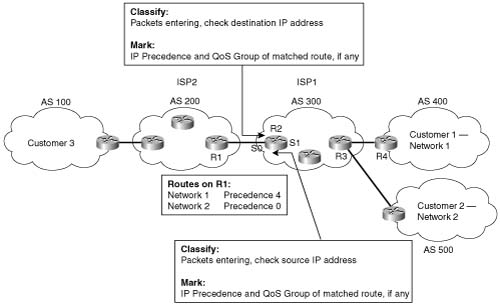
ISPs may want a QoS policy just to prefer one customer’s traffic over another. In Figure B-9, for instance, consider ISP 1, which has two customers. Customer 1 has agreed to pay a premium for its Internet service, in return for ISP 1 agreeing to provide better latency and delay characteristics for the traffic. Customer 2 keeps paying the same amount as always, and still gets best- effort service.
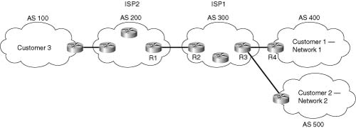
The QoS tools only need to differentiate between Customer 1 and Customer 2 traffic to support this policy. So, for packets flowing from right to left, if the source IP address is an IP address in Customer 1’s network, the packet might be marked with precedence 4, for instance. Similarly, when packets flow left to right, these same tools could examine the destination IP address, and if it’s part of Customer 1’s network, precedence 4 could be marked. Packets to or from Customer 2 could be marked with precedence 0.
Class-based (CB) marking, policy-based routing (PBR), and committed access rate (CAR) could perform the necessary marking to support premium and best-effort customer services. However, each of these three tools has some negative side effects. For all three tools, that classification would require an IP ACL for matching the packets, for all packets. For an ISP with many customers, however, classifying and marking packets based on referencing ACLs for a large number of packets may induce too much overhead traffic. Suppose further that ISP 1 and ISP 2 agree to support each other’s premium and best-effort customers in a similar manner. The two ISP’s would have to continually exchange information about which networks are premium, and which are not, if they are using IP ACLs to classify the traffic. Additionally, when new customers are added, ISP 1 may be waiting on ISP 2 to update their QoS configuration before the desired level of service is offered to the new customer.
To overcome the two issues—the scalability of classifying based on ACLs, and the administrative problems of just listing the networks that need premium services—QPPB was created. QPPB allows marking of packets based on an IP precedence or QoS group value associated with a Border Gateway Protocol (BGP) route. For instance, the BGP route for Customer 1’s network, Network A, could be given a BGP path attribute that both ISP 1 and ISP 2 agree should mean that this network receives better QoS service. Because BGP already advertises the routes, and the QoS policy is based on the networks described in the routes, QPPB marking can be done more efficiently than with the other classification and marking tools.
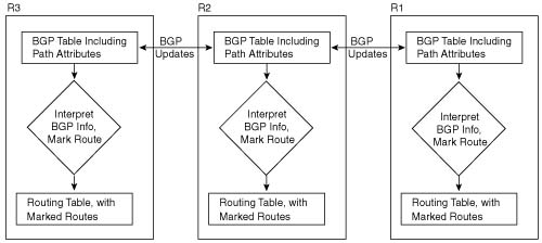
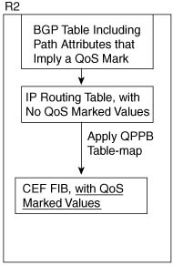
Figure B-10 shows the basic process in action. In this example, R3 is configured to use QPPB, although it would likely be used in several places around the network.
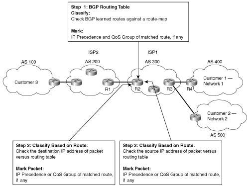
QPPB follows two steps: marking routes, and then marking packets based on the values marked on the routing entries. BGP routing information includes the network numbers used by the various customers, and other BGP path attributes. Because Cisco has worked hard over the years to streamline the process of table lookup in the routing table, to reduce per-packet processing for the forwarding process, QPPB can use this same efficient table-lookup process to reduce classification and marking overhead.
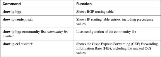
For reference, Tables B-8 and B-9 summarize the QPPB configuration and exec commands, respectively.
QPPB can be a confusing topic. The rest of this section discusses more detail about how QPPB works and how to configure it. One key to understanding QPPB, in spite of some of the detail, is to keep these two key points in mind as you read the following sections:
![]() QPPB classifies BGP routes based on the BGP routes’ attributes, and marks BPG routes with an IP precedence or QoS group value.
QPPB classifies BGP routes based on the BGP routes’ attributes, and marks BPG routes with an IP precedence or QoS group value.
![]() QPPB classifies packets based on the associated routing table entries, and marks the packets based on the marked values in the routing table entry.
QPPB classifies packets based on the associated routing table entries, and marks the packets based on the marked values in the routing table entry.
Because QPPB involves quite a few detailed concepts and configuration, some of the true details of how QPPB works are glossed over during the initial discussions. These details are explained at the end of this section in the subsection titled “QPPB: The Hidden Details.”
QPPB allows routers to mark packets based on information contained in the routing table. Before packets can be marked, QPPB first must somehow associate a particular marked valued with a particular route. QPPB, as the name implies, accomplishes this task using BGP. This first step can almost be considered as a separate classification and marking step by itself, because BGP routes are classified, based on information that describes the route, and marked with some QoS value.
The classification feature of QPPB can examine many of the BGP path attributes. The two most useful BGP attributes for QPPB are the autonomous system number (ASN) sequence, referred to as the autonomous system path, and the community string. The autonomous system path contains the ordered list of ASNs, representing the ASNs between a router and the autonomous system of the network described in the route. In Figure B-10, R1 receives a BGP update for Network 1, listing ASNs 300 and 400 in the autonomous system path and a BGP update for Network 2, listing ASNs 300 and 500 in the autonomous system path. QPPB can be used to mark the route to Network 1 (Customer 1) with one precedence value, while marking the route to Network 2 (Customer 2) with another precedence value, based on the autonomous system path received for the route to each customer.
The community attribute provides a little more control than does the autonomous system path. The autonomous system path is used to avoid routing loops, and the contents of the autonomous system path changes when aggregate routes are formed. The community attribute, however, allows the engineer to essentially mark any valid value. For instance, R3 could set the community attribute to 10:200 for the route to Network 1, and advertise that route toward the left side of the network diagram. Other routers could then use QPPB to classify based on the community attribute of 10:200, and assign the appropriate precedence value to the route to Network 1. QPPB configuration would essentially create logic as follows: “If the community attribute contains 10:200, mark the route with precedence 4.”
Example B-10 lists the QPPB configuration just for marking the route based on the autonomous system number. With this configuration, no packets are marked, because the QPPB configuration is not complete. (The complete configuration appears in the next section.) QPPB is a two- step process, and Example B-1 just shows the configuration for the first step.
Example B-10 QPPB Route Marking with BGP Table Map: R2
table-map mark-prec4-as400
!
route-map mark-prec4-as400 10
match as-path 1
set ip precedence 4
!
route-map mark-prec4-as400 20
set ip precedence 0
!
ip as-path access-list 1 permit _400_
This example shows R2’s configuration for QPPB. (Note that the entire BGP configuration is not shown, just the configuration pertinent to QPPB.) The table-map BGP router subcommand tells IOS that, before adding BGP routes to the routing table, it should examine a route map called mark-prec4-as400. Based on the match and set commands in the route map, when BGP adds routes to the routing table, it also associates either precedence 4 or precedence 0 with each route.
The route map has two clauses—one that matches routes that have autonomous system 400 anywhere in the autonomous system path sequence attribute, and a second clause that matches all routes. Clause 10 matches ASN 400 by referring to autonomous system path ACL 1, which matches any autonomous system path containing ASN 400, and sets the precedence to 4 for those routes. Clause 20 matches all packets, because no specific match command is configured, and sets the precedence to 0.
After QPPB has marked routes with IP precedence or QoS group values, the packet marking part must be performed. After the packets have been marked, traditional QoS tools can be used to perform queuing, congestion avoidance, policing, and so on, based on the marked value.
QPPB’s packet-marking logic flows as follows:
1. Process packets entering an interface.
2. Match the destination or source IP address of the packet to the routing table.
3. Mark the packet with the precedence or QoS group value shown in the routing table entry.
The three-step logic for QPPB packet marking follows the same general flow as the other classification and marking tools; in this case, however, the classification options, and the marking options, are quite limited. QPPB packet classification is based on the routing table entry that matches the packet, and QPPB packet marking just marks the packet with the same value found marked in the route.
Figure B-11 shows with the same network, but with the marking logic on R2 shown.
QPPB allows for marking of packets that have been sent to Customer 1, and for marking packets that have been sent by Customer 1. For packets entering R2’s S0 interface, for instance, the packet is going toward Customer 1, so the destination IP address is in Network 1. Therefore, the QPPB logic on R2’s S0 should compare the packet’s destination IP address to the routing table; if the appropriate QoS field has been set in the route, the packet is marked with the same value. That takes care of packets passing through R3 that are headed to Customer 1.
For packets that Customer 1 has sent, going from right to left in the figure, QPPB on R2 can still mark the packets. These packets typically enter R2’s S1 interface, however, and the packets have a source IP addresses in Network 1. To associate these packets with Network 1, QPPB examines the routing table entry that matches the packet’s source IP address. This match of the routing table is not used for packet forwarding; it is used only for finding the precedence or the QoS group value to set on the packet. In fact, the table lookup for destination addresses does not replace the normal table lookup for forwarding the packet, either. Because the routing table entry for Network 1 has IP precedence set to 4, QPPB marks these packets with precedence 4.
Example B-11 shows the completed configuration on R2, with the additional configuration for per-packet marking highlighted.
Example B-11 QPPB: Completed Example on R2
!
Router bgp 300
table-map mark-prec4-as400
!
route-map mark-prec4-as400 10
match as-path 1
set ip precedence 4
!
route-map mark-prec4-as400 20
set ip precedence 0
!
ip as-path access-list 1 permit _400_
!
interface Serial0
bgp-policy destination ip-prec-map
!
interface serial1
bgp-policy source ip-prec-map
The bgp-policy interface subcommand enables QPPB for packets entering the interface. The destination or source keyword identifies whether QPPB should perform table lookup on the packets’ destination or source addresses, respectively. On S0, the destination keyword is used, because the packets entering S0 presumably are going toward Customer 1. Conversely, on S1 the source keyword is used, because the packets entering S1 presumably were sent by Customer 1. Finally, the ip-prec-map keyword implies that the precedence should be set based on the routing table entry, and not the QoS group.
QPPB can classify based on both the autonomous system path and the community string. BGP considers the autonomous system path as a well-known mandatory path attribute; therefore, in the earlier examples, R3 could just examine the autonomous system path. Conversely, BGP considers the community string to be an optional transitive attribute—which means that the community string does not have to be set, and is not set without some additional configuration causing it to be set.
Example B-12 shows the same network, with the same goal of giving Customer 1 premium service. In this example, however, the BGP community attribute is used. The community attribute is set by R3, for routes received from Customer 1 via BGP. With the community attribute set, other routers can use it for classifying the BGP routes and marking the routes with precedence 4. The example shows R3’s QPPB configuration. Example B-12 lists the configuration on R3, and Example B-13 lists the configuration on R2.
Example B-12 QPPB Sample Based on BGP Community: R3 Configuration
neighbor 192.168.1.1 remote-as 400
neighbor 192.168.1.1 route-map set-comm in
neighbor 192.168.2.2 remote-as 300
neighbor 192.168.2.2 send-community
!
route-map set-comm permit 10
set community 4:50
Example B-13 QPPB Sample Based on BGP Community: R2 Configuration
!
router bgp 300
table-map mark-prec4-comm
!
route-map mark-prec4-comm permit 10
match community 1
set ip precedence 4
!
route-map mark-prec4-comm permit 20
set ip precedence 0
!
ip community-list 1 permit 4:50
!
interface Serial0
bgp-policy destination ip-prec-map
!
interface serial1
bgp-policy source ip-prec-map
In Example B-12, R3 has just set the community string to 4:50 for BGP routes learned from neighbor 192.168.1.1, which is a router at Customer 1. To set the community, BGP uses route-map set-comm based on the neighbor 192.168.1.1 route-map set-comm in command. This route map contains 1 clause, which matches all routes because there is no match command in clause 10, and sets the community string to 4:50. IOS BGP does not forward the community attribute by default, so the neighbor 192.168.2.2 send-community command is needed to make R3 send the community string to R2, whose BGP ID is 192.168.2.2. So, R3 has set all incoming routes from R4 with community 4:50, and includes the community attribute in the updates sent to R2.
Example B-13 shows the configuration for QPPB on R2. The configuration is similar to Example B-11, with the highlighted sections pointing out the added or changed configuration. The table-map BGP router subcommand still directs BGP to mark the routes with precedence 4, but this time using a new route map, mark-prec4-comm. This route map uses two clauses. The first clause, clause 10, matches the community set by R3 by referring to IP community list 1 using the match community 1 command. The community list, created in the single global command ip community-list 1 permit 4:50, just matches all BGP routes whose community string contains 4:50. Route map mark-prec4-comm sets IP precedence 4 for BGP routes that match the community sting. The second route map clause, clause 20, matches all routes because no explicit match statement is configured, and sets the IP precedence to 0 for these routes.
The packet-marking function, as opposed to the route-marking function, is enabled by the bgp-policy interface subcommands, which are exactly the same as shown earlier in Example B-6.
As mentioned earlier, QPPB confuses most people the first time they learn about it. Therefore, you should understand a bit more about it. The first aspect of QPPB you should understand pertains to what BGP updates contain in support of QPPB, and the second aspect of QPPB you should understand is what really happens when QPPB marks a route.
First, BGP updates do not include the IP precedence or QoS group value inside the BGP update. QPPB reacts to the information in a normal BGP update to perform QoS marking of BGP routes, and then in turn performs packet marking based on the marked routes. In other words, BGP RFCs did not add any specification for adding a QoS marking field to the information inside the update. Therefore, to mark based on BGP routes, QPPB uses preexisting fields in the BGP update, such as the autonomous system path and the community attribute. In fact, the BGP-4 RFCs added the community attribute to provide a flexible field for marking BGP routes for future unforeseen purposes, such as QPPB. Figure B-12 depicts the general idea:
When marking IP precedence in packets, QPPB marks the same field already covered in depth in this chapter—the first 3 bits of the ToS byte. When QPPB marks the QoS group, it actually marks a header that is added to the packet when passing through a 7500, GSR, or ESR series router. However, QPPB must mark the route first, and then mark the packet based on the route that matches the source or destination IP address in the packet. To understand what mark the route really means, you must take at least a cursory look at Cisco Express Forwarding (CEF).
IOS provides several different processing paths in software for forwarding packets. Process switching is one of those paths, and is the most processor-intensive path. Fast switching is another switching path still in use today. CEF is yet another switching or forwarding path, and CEF has been designed to be very efficient. Other switching paths have also been added over the years, some specific to particular hardware models. The one thing all these optimized forwarding paths have in common is that they optimize for the forwarding process by streamlining two functions: the process of matching the correct route in the routing table, and the process of building and adding the new data-link header to the packet.
CEF optimizes forwarding by creating a new table that includes entries for the routes in the routing table. This table is called the Forwarding Information Base (FIB). The FIB optimizes the process of locating a route by performing a table lookup in the FIB rather than the less- efficient table lookup of the routing table. In other words, CEF switching crunches the routing table into the FIB, and then uses the FIB to make the forwarding decisions. (This in itself is somewhat of an oversimplification of CEF; for more detail, refer to Vijay Bollapragada’s Inside Cisco IOS Software Architecture [Cisco Press, 2000].)
CEF optimizes the creation of new data-link headers by creating a table that contains the new data-link header associated with each next-hop IP address in the FIB. By doing so, when FIB table lookup is complete, the header can be added to the packet with little processing.
When QPPB marks a route, it actually marks either or both of the two fields inside each entry in the FIB. The FIB contains IP precedence and QoS group fields in order to support QPPB. Therefore, when CEF crunches the routing table to create FIB entries, when QPPB is configured, the appropriate FIB precedence and QoS group fields are set. Figure B-13 shows the general idea.
This section covers PQ and CQ configuration, as well as distributed WFQ (dWFQ) and MDRR configuration.
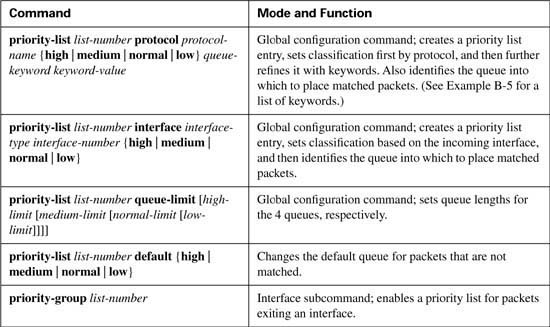
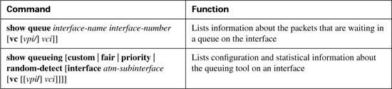
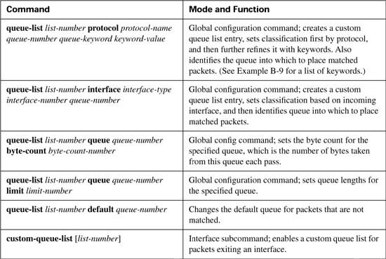
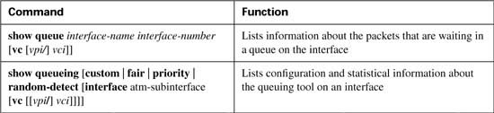
PQ configuration resembles access-control list (ACL) configuration, except the result is to queue a packet rather than discarding it. Global commands are used to define the logic for classifying packets by matching header fields, and an interface subcommand is used to enable PQ on an interface. Example configurations for PQ follow Tables B-10 and B-11, which list the configuration and exec commands related to PQ, respectively.
To understand the core PQ configuration commands, examine Example B-14. In this example, R3 uses PQ on its S0/0 interface. The engineer configuring R3 decided that voice traffic could benefit from being placed into the High queue, so a simple QoS policy has been devised:
![]() All VoIP payload traffic is placed in the High queue.
All VoIP payload traffic is placed in the High queue.
![]() All other traffic is placed in the Normal queue.
All other traffic is placed in the Normal queue.
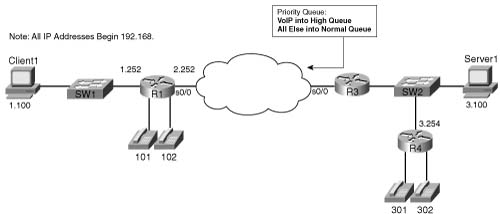
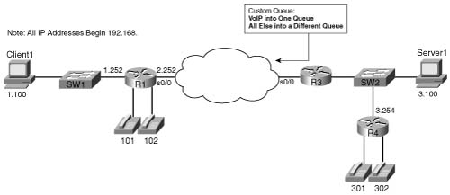
Figure B-14 shows the network in which the configuration is applied, and Example B-14 shows the configuration and the commands used. Note that all IP addresses in the example start with 192.168.
Example B-14 Priority Queuing, VoIP in High Queue, All Else in Normal Queue
Building configuration...
! Portions omitted for brevity
interface Ethernet0/0
description connected to SW2, where Server1 is connected
ip address 192.168.3.253 255.255.255.0
load-interval 30
!
interface Serial0/0
description connected to FRS port S0. Single PVC to R1.
no ip address
encapsulation frame-relay
load-interval 30
priority-group 5
clockrate 64000
!
interface Serial0/0.1 point-to-point
description point-point subint global DLCI 103, connected via PVC to DLCI 101 (R1)
ip address 192.168.2.253 255.255.255.0
frame-relay interface-dlci 101
!
access-list 120 permit udp any range 16384 32767 any range 16384 32767
!
priority-list 5 protocol ip high list 120
Output queue for Serial0/0 is 26/60
Packet 1, linktype: ip, length: 1404, flags: 0x88
source: 192.168.3.100, destination: 192.168.1.100, id: 0xF560, ttl: 127,
TOS: 0 prot: 6, source port 2831, destination port 1668
data: 0x0B0F 0x0684 0x79EB 0x0D2A 0x05B4 0x0FF5 0x5010
0x4510 0x5BF8 0x0000 0x6076 0xEEFD 0xFBB6 0xCC72
Packet 2, linktype: ip, length: 724, flags: 0x88
source: 192.168.3.100, destination: 192.168.1.100, id: 0xF561, ttl: 127,
TOS: 0 prot: 6, source port 80, destination port 1667
data: 0x0050 0x0683 0x79C1 0x0930 0x05B3 0xE88E 0x5010
0x41C5 0x276E 0x0000 0xDA9B 0x48F7 0x7F64 0x7313
Packet 3, linktype: ip, length: 724, flags: 0x88
source: 192.168.3.100, destination: 192.168.1.100, id: 0xF562, ttl: 127,
TOS: 0 prot: 6, source port 80, destination port 1666
data: 0x0050 0x0682 0x79BC 0xE875 0x05B3 0xE2C6 0x5010
0x441A 0xA5A2 0x0000 0x8071 0x4239 0x5906 0xD18C
! Several lines omitted for brevity
R3#show queueing interface serial 0/0
Interface Serial0/0 queueing strategy: priority
Output queue utilization (queue/count)
high/13593 medium/0 normal/206 low/0
R3#show queueing priority
Current DLCI priority queue configuration:
Current priority queue configuration:
List Queue Args
5 high protocol ip list 120
R3#show int s 0/0
Serial0/0 is up, line protocol is up
Hardware is PowerQUICC Serial
Description: connected to FRS port S0. Single PVC to R1.
MTU 1500 bytes, BW 1544 Kbit, DLY 20000 usec,
reliability 255/255, txload 9/255, rxload 8/255
Encapsulation FRAME-RELAY, loopback not set
Keepalive set (10 sec)
LMI enq sent 79, LMI stat recvd 70, LMI upd recvd 0, DTE LMI up
LMI enq recvd 0, LMI stat sent 0, LMI upd sent 0
Broadcast queue 0/64, broadcasts sent/dropped 165/2, interface broadcasts 149
Last input 00:00:02, output 00:00:00, output hang never
Last clearing of "show interface" counters 00:13:25
Input queue: 0/75/0/0 (size/max/drops/flushes); Total output drops: 2
Queueing strategy: priority-list 5
Output queue (queue priority: size/max/drops):
high: 4/20/2, medium: 0/40/0, normal: 20/60/0, low: 0/80/0
!
! Lines omitted for brevity.
Example B-14 uses only one priority-list command in this case, putting voice traffic into the High queue and letting the rest of the traffic be placed in the Normal queue by default. The priority-list 5 protocol ip high list 120 command matches all IP packets that are permitted by ACL 120, which matches all VoIP User Datagram Protocol (UDP) ports. The priority-group 5 interface subcommand enables PQ on S0/0, linking PQ list 5 with the interface.
Two similar commands display some limited information about PQ. First, the show queue command lists brief information about packets currently in the queue. Notice that some information is listed for each packet in the queue; in Example B-14, a packet that was sent by the web server (source port 80) is highlighted. Also note that none of the stanzas describing the packets in the queue shows a voice packet, with UDP ports between 16384 and 32767. Because PQ always serves the High queue first, you would need to have more voice traffic being sent into the network than the speed of the interface before packets would ever actually back up into the High queue. Therefore, it is rare to see queue entries for packets in the High queue.
The show queueing interface command lists configuration information about PQ and statistical information about how many packets have been placed into each queue. Note that no packets have been placed into the Medium or Low queues, because priority-list 5 matches VoIP packets, placing them in the High queue, with all other packets defaulting to the Normal queue. The show queueing priority command lists information about the configuration of PQ.
Finally, the output of the show interfaces command states that PQ is in use, along with statistics about each queue. The current number of packets in each queue, the maximum length of each queue, and the cumulative number of tail drops is listed for each of the four queues.
Good QoS design calls for the marking of packets close to the source of the packet. The next example (Example B-15) accomplishes the same queuing goals as the preceding example, but in this case, PQ relies on the fact that the packets have been marked before reaching R3’s S0/0 interface. In a real network, the packets could be marked on one of the LAN switches, or in an IP Phone, or by the computers in the network. This example shows the packets being marked upon entering R3’s E0/0 interface. Example B-15 shows the revised configuration based on the following criteria:
![]() All VoIP payload traffic has been marked with DSCP EF; place this traffic in the High queue.
All VoIP payload traffic has been marked with DSCP EF; place this traffic in the High queue.
![]() All other traffic has been marked with DSCP BE; place this traffic in the Normal queue.
All other traffic has been marked with DSCP BE; place this traffic in the Normal queue.
Example B-15 Priority Queuing, DSCP EF in High Queue, All Else in Normal Queue
! Portions omitted for brevity
! Next several lines are CB Marking configuration, not PQ configuration
class-map match-all all-else
match any
class-map match-all voip-rtp
match ip rtp 16384 16383
!
policy-map voip-and-be
class voip-rtp
set ip dscp 46
class class-default
set ip dscp 0
!
!
interface Ethernet0/0
description connected to SW2, where Server1 is connected
ip address 192.168.3.253 255.255.255.0
load-interval 30
service-policy input voip-and-be
!
interface Serial0/0
description connected to FRS port S0. Single PVC to R1.
no ip address
encapsulation frame-relay
load-interval 30
priority-group 6
clockrate 128000
!
interface Serial0/0.1 point-to-point
description point-point subint global DLCI 103, connected via PVC to DLCI 101 (R1)
ip address 192.168.2.253 255.255.255.0
frame-relay interface-dlci 101
!
! Portions omitted for brevity
!
access-list 121 permit ip any any dscp ef
!
priority-list 6 protocol ip high list 121
! Portions omitted for brevity
R3#show queueing priority
Current DLCI priority queue configuration:
Current priority queue configuration:
List Queue Args
6 high protocol ip list 121
R3#show interface s 0/0
Serial0/0 is up, line protocol is up
Hardware is PowerQUICC Serial
Description: connected to FRS port S0. Single PVC to R1.
MTU 1500 bytes, BW 1544 Kbit, DLY 20000 usec,
reliability 255/255, txload 20/255, rxload 6/255
Encapsulation FRAME-RELAY, loopback not set
Keepalive set (10 sec)
LMI enq sent 29, LMI stat recvd 29, LMI upd recvd 0, DTE LMI up
LMI enq recvd 0, LMI stat sent 0, LMI upd sent 0
LMI DLCI 1023 LMI type is CISCO frame relay DTE
Broadcast queue 0/64, broadcasts sent/dropped 68/0, interface broadcasts 63
Last input 00:00:01, output 00:00:00, output hang never
Last clearing of "show interface" counters 00:04:50
Input queue: 0/75/0/0 (size/max/drops/flushes); Total output drops: 751
Queueing strategy: priority-list 6
Output queue (queue priority: size/max/drops):
high: 0/20/0, medium: 0/40/0, normal: 4/60/751, low: 0/80/0
!
!Portions omitted for brevity.
In Example B-15, priority-list 6 contains a single entry, referring to ACL 121, which matches all IP packets with DSCP EF. The priority-group 6 command enables PQ on S0/0. Before the PQ configuration can actually do what the requirements suggest, the packets must be marked. The policy-map voip-and-be command matches VoIP packets based on their UDP port numbers, and marks them on ingress to interface e0/0. Note that unlike the preceding example, when an ACL matched all UDP ports between 16384 and 32767, this example matches only even- numbered ports, which are the ports actually used for VoIP payload. (The odd-numbered ports are used for voice signaling.) The match ip rtp 16384 16383 command matches the same range of port numbers as ACL 120, except it only matches the even (payload) ports.
PQ can only support four different classifications of packets, because it only has four queues. Example B-16 shows all four queues being used. The following criteria is used for queuing packets on R3’s S0/0 interface:
![]() VoIP payload is placed into the High queue.
VoIP payload is placed into the High queue.
![]() NetMeeting voice and video from Server1 to Client1 is placed in the Medium queue.
NetMeeting voice and video from Server1 to Client1 is placed in the Medium queue.
![]() Any HTTP traffic is placed into the Normal queue.
Any HTTP traffic is placed into the Normal queue.
![]() All other traffic is placed into the low queue.
All other traffic is placed into the low queue.
The same network used in the preceding example, as shown in Figure B-14, is used for this example, too.
Example B-16 PQ Example: VoIP in High, NetMeeting in Medium, HTTP in Normal, and All Else in Low Queue
range 16384 32767
!
access-list 151 permit udp any range 16384 32768 any range 16384 32768
!
access-list 152 permit tcp any eq www any
access-list 152 permit tcp any any eq www
!
priority-list 8 protocol ip medium list 150
priority-list 8 protocol ip high list 151
priority-list 8 protocol ip normal list 152
priority-list 8 default low
!
interface serial 0/0
priority-group 8
Note a couple of points from the example. First, there is no need to match the traffic that goes into the Low queue, because the priority-list 8 default low command makes the Low queue the default queue for unmatched packets. Second, note that ACL 152 matches web traffic from web servers, as well as to web servers. In this limited example, you only needed to check for packets from the web server when performing queuing on output of R3’s S0/0 interface. Because one day you might have traffic going to a web server exiting R3’s S0/0 interface, however, you might want to go ahead and match all web traffic as shown in the ACL.
Finally, one last example shows the equivalent configuration as shown in Example B-16, but with the assumption that the traffic had been marked before reaching R3’s S0/0 interface. Again, the packets are marked upon entering R3’s E0/0, using CB marking. The criteria used for the final example, whose configuration is shown in Example B-17, is as follows:
![]() VoIP payload is marked with DSCP EF (decimal 46); put this traffic in the High queue.
VoIP payload is marked with DSCP EF (decimal 46); put this traffic in the High queue.
![]() NetMeeting voice and video from Server1 to Client1 has been marked with DSCP AF41 (decimal 34); place this traffic in the Medium queue.
NetMeeting voice and video from Server1 to Client1 has been marked with DSCP AF41 (decimal 34); place this traffic in the Medium queue.
![]() Any HTTP traffic has been marked with DSCP AF22 (decimal 20); place this traffic in the Normal queue.
Any HTTP traffic has been marked with DSCP AF22 (decimal 20); place this traffic in the Normal queue.
![]() All other traffic has been marked with DSCP BE (decimal 0); place this traffic in the Low queue.
All other traffic has been marked with DSCP BE (decimal 0); place this traffic in the Low queue.
Example B-17 PQ Example: DSCP EF in High, DSCP AF41 in Medium, DSCP AF22 in Normal, and All Else in Low Queue
! Portions omitted for brevity
class-map match-all http-all
match protocol http
class-map match-all voip-rtp
match ip rtp 16384 16383
class-map match-all NetMeet
match access-group NetMeet-ACL
class-map match-all all-else
match any
!
policy-map laundry-list
class voip-rtp
set ip dscp 46
class NetMeet
set ip dscp 34
class http-all
set ip dscp 20
class class-default
set ip dscp 0
!
interface Ethernet0/0
description connected to SW2, where Server1 is connected
ip address 192.168.3.253 255.255.255.0
ip nbar protocol-discovery
load-interval 30
service-policy input laundry-list
!
interface Serial0/0
description connected to FRS port S0. Single PVC to R1.
no ip address
encapsulation frame-relay
priority-group 7
clockrate 128000
!
interface Serial0/0.1 point-to-point
description point-point subint global DLCI 103, connected via PVC to DLCI 101 (R1)
ip address 192.168.2.253 255.255.255.0
frame-relay interface-dlci 101
!
ip access-list extended NetMeet-ACL
permit udp host 192.168.3.100 range 16384 32768192.168.1.0 0.0.0.255 range 16384 32768
!
access-list 130 permit ip any any dscp ef
access-list 131 permit ip any any dscp af41
access-list 132 permit ip any any dscp af22
access-list 133 permit ip any any dscp default
!
priority-list 7 protocol ip high list 130
priority-list 7 protocol ip medium list 131
priority-list 7 protocol ip normal list 132
priority-list 7 protocol ip low list 133
priority-list 7 default low
R3#show queueing int s 0/0
Interface Serial0/0 queueing strategy: priority
Output queue utilization (queue/count)
high/42092 medium/1182 normal/52 low/3242
As seen in Example B-17, if the packets have already been marked, PQ can simply match the DSCP field. Routers that forward these packets later can also just configure PQ, and match the DSCP field. Note that PQ needs to refer to an ACL to match the DSCP field, whereas some other queuing tools can refer directly to the DSCP field without using an ACL. Another interesting point to note in this configuration is that the CB marking configuration used network-based application recognition (NBAR) with the match protocol http command to match all web traffic, and then set those packets with DSCP 20. Example B-16 showed why you might want to match all web traffic, but the configuration used two entries to match all web traffic (ACL 152). With NBAR, you can match all web traffic, regardless of whether it is coming from or going to a web server.
CQ configuration resembles PQ configuration. Global commands are used to define the logic for classifying packets by matching header fields, and an interface subcommand is used to enable CQ on an interface. Example configurations for CQ follow Tables B-12 and B-13, which list the configuration and exec commands related to CQ, respectively.
To understand the core CQ configuration commands, examine Example B-18. (This example is identical to Example B-14, shown in the “PQ Configuration” section earlier in this chapter, except that CQ is used rather than PQ.) In this example, R3 uses CQ on its S0/0 interface. The engineer configuring R3 decided that voice traffic could benefit from being given preferential queuing treatment, so a simple QoS policy has been devised, as noted in the following:
![]() All VoIP payload traffic is placed in Queue 2.
All VoIP payload traffic is placed in Queue 2.
![]() All other traffic is placed in Queue 1.
All other traffic is placed in Queue 1.
![]() Assign about 2/3 of the bandwidth to the VoIP traffic.
Assign about 2/3 of the bandwidth to the VoIP traffic.
Figure B-15 shows the network in which the configuration is applied, and Example B-18 shows the configuration and show commands:
Example B-18 Custom Queuing: VoIP in High Queue, All Else in Normal Queue
fragments Prioritize fragmented IP packets
gt Classify packets greater than a specified size
list To specify an access list
lt Classify packets less than a specified size
tcp Prioritize TCP packets 'to' or 'from' the specified port
udp Prioritize UDP packets 'to' or 'from' the specified port
<cr>
R3(config)#^Z
R3#show running-config
access-list 120 permit udp any range 16383 32767 any range 16383 32767
!
queue-list 5 protocol ip 2 list 120
queue-list 5 queue 1 byte-count 2500
queue-list 5 queue 2 limit 30
!
interface serial0/0
custom-queue-list 5
!
R3#show queueing custom
Current custom queue configuration:
List Queue Args
5 2 protocol ip list 120
5 1 byte-count 2500
5 2 byte-count 5000 limit 30
R3#show queueing int s 0/0
Interface Serial0/0 queueing strategy: custom
Output queue utilization (queue/count)
0/15 1/91 2/3549 3/0 4/0 5/0 6/0 7/0 8/0
9/0 10/0 11/0 12/0 13/0 14/0 15/0 16/0
R3#show int s 0/0
Serial0/0 is up, line protocol is up
Hardware is PowerQUICC Serial
Description: connected to FRS port S0. Single PVC to R1.
MTU 1500 bytes, BW 1544 Kbit, DLY 20000 usec,
reliability 255/255, txload 9/255, rxload 8/255
Encapsulation FRAME-RELAY, loopback not set
Keepalive set (10 sec)
LMI enq sent 1, LMI stat recvd 1, LMI upd recvd 0, DTE LMI up
LMI enq recvd 0, LMI stat sent 0, LMI upd sent 0
LMI DLCI 1023 LMI type is CISCO frame relay DTE
Broadcast queue 0/64, broadcasts sent/dropped 4/0, interface broadcasts 3
Last input 00:00:00, output 00:00:00, output hang never
Last clearing of "show interface" counters 00:00:12
Input queue: 0/75/0/0 (size/max/drops/flushes); Total output drops: 282
Queueing strategy: custom-list 5
Output queues: (queue #: size/max/drops)
0: 0/20/0 1: 6/20/0 2: 28/30/282 3: 0/20/0 4: 0/20/0
5: 0/20/0 6: 0/20/0 7: 0/20/0 8: 0/20/0 9: 0/20/0
10: 0/20/0 11: 0/20/0 12: 0/20/0 13: 0/20/0 14: 0/20/0
15: 0/20/0 16: 0/20/0
5 minute input rate 52000 bits/sec, 102 packets/sec
5 minute output rate 60000 bits/sec, 73 packets/sec
1394 packets input, 89409 bytes, 0 no buffer
Received 0 broadcasts, 0 runts, 0 giants, 0 throttles
0 input errors, 0 CRC, 0 frame, 0 overrun, 0 ignored, 0 abort
The configuration for this scenario only requires a few commands. The queue-list 5 protocol ip 2 list 120 command causes CQ to match all packets permitted by ACL 120 and to place these packets into Queue 2. CQ uses Queue 1 for unmatched packets, so no other classification commands are required. The byte count for each queue defaults to 1500 bytes; in this case, the criteria specified that CQ should give about 2/3 of the bandwidth to the VoIP traffic, so queue 2 was assigned a byte count of 5000, and Queue 1 a byte count of 2500. At a 64-kbps clock rate, each complete cycle takes a little less than a second. Finally, to enable CQ list 5, the custom- queue interface subcommand was used.
IOS uses the same show commands to display information about CQ as it does for PQ. The show queue command lists brief information about packets in the queue at the present time (not shown in the example). The show queueing interface command lists configuration information about CQ and statistical information about how many packets have been placed into each queue. In the example, Queue 2 has had a total of 3549 packets pass through it. Also note that no packets have been placed into Queues 3 through 16, because CQ list 5 does not classify packets into Queues 3 through 16. The show queueing custom command lists information about the configuration of CQ. The output of the show interfaces command states that CQ is in use, along with statistics about each queue. The current number of packets in each queue, the maximum length of each queue, and the cumulative number of tail drops are listed for each of the 16 queues.
You may have noticed that Queue 0 shows up in a couple of commands. CQ uses a special queue, Queue 0, which is used for important high-priority packets generated by the router. Routing protocol updates are considered high priority, for instance, so these packets are placed into Queue 0. CQ treats Queue 0 as a priority queue—that is, when packets are waiting in Queue 0, CQ interrupts its normal scheduling logic, takes the packet from Queue 0 next, and then resumes the scheduling process. CQ does not allow packets to be explicitly classified into Queue 0.
Stepping back from the configuration for a moment, consider the time required to service 2500 bytes from Queue 1, and then 5000 bytes from Queue 2, at 64 kbps. It requires roughly .875 seconds total, with roughly 310 ms to service Queue 1, and the rest to service Queue 2. So, if Queue 1 has many packets, the voice packet in Queue 2 that is the next packet to get serviced, after Queue 1 gets to send its 2500 bytes, has to wait an extra 310 ms! So, this example, although giving voice 2/3 of the bandwidth, does not actually give voice very good performance.
Good QoS design calls for the marking of packets close to the source of the packet. The next example accomplishes the same queuing goals as the preceding example, but CQ relies on the fact that the packets have been marked before reaching R3’s S0/0 interface. In a real network, the packets could be marked on one of the LAN switches; for review, however, this example shows the packets being marked upon entering R3’s E0/0 interface. Example B-19 shows the revised configuration based on the following criteria:
![]() All VoIP payload traffic has been marked with DSCP EF; place this traffic in Queue 1.
All VoIP payload traffic has been marked with DSCP EF; place this traffic in Queue 1.
![]() All other traffic has been marked with DSCP BE; place this traffic in Queue 2.
All other traffic has been marked with DSCP BE; place this traffic in Queue 2.
![]() VoIP traffic is given about 2/3 of the bandwidth.
VoIP traffic is given about 2/3 of the bandwidth.
Example B-19 Custom Queuing: DSCP EF in Queue 1, All Else in Queue 2
!
class-map match-all class-default
match any
class-map match-all voip-rtp
match ip rtp 16384 16383
!
!
policy-map voip-and-be
class voip-rtp
set ip dscp 46
class all-else
set ip dscp 0
!
interface Ethernet0/0
service-policy input voip-and-be
!
interface Serial0/0
custom-queue-list 6
clockrate 64000
!
interface Serial0/0.1 point-to-point
description point-point subint global DLCI 103, connected via PVC to DLCI 101 (R1)
ip address 192.168.2.253 255.255.255.0
frame-relay interface-dlci 101
!
! Portions omitted for brevity
!
access-list 121 permit ip any any dscp ef
!
queue-list 6 protocol ip 1 list 121
queue-list 6 queue 2 byte-count 2500
queue-list 6 default 2
R3#sh queueing int s 0/0
Interface Serial0/0 queueing strategy: custom
Output queue utilization (queue/count)
0/5 1/1012 2/30 3/0 4/0 5/0 6/0 7/0 8/0
9/0 10/0 11/0 12/0 13/0 14/0 15/0 16/0
R3#show queueing custom
Current custom queue configuration:
List Queue Args
6 2 default
6 1 protocol ip list 121
6 1 byte-count 5000
6 2 byte-count 2500
R3#show int s 0/0
Serial0/0 is up, line protocol is up
Hardware is PowerQUICC Serial
Description: connected to FRS port S0. Single PVC to R1.
MTU 1500 bytes, BW 1544 Kbit, DLY 20000 usec,
reliability 255/255, txload 10/255, rxload 8/255
Encapsulation FRAME-RELAY, loopback not set
Keepalive set (10 sec)
LMI enq sent 4, LMI stat recvd 4, LMI upd recvd 0, DTE LMI up
LMI enq recvd 0, LMI stat sent 0, LMI upd sent 0
LMI DLCI 1023 LMI type is CISCO frame relay DTE
Broadcast queue 0/64, broadcasts sent/dropped 7/0, interface broadcasts 7
Last input 00:00:02, output 00:00:00, output hang never
Last clearing of "show interface" counters 00:00:33
Input queue: 0/75/0/0 (size/max/drops/flushes); Total output drops: 718
Queueing strategy: custom-list 6
Output queues: (queue #: size/max/drops)
0: 0/20/0 1: 16/20/718 2: 19/20/0 3: 0/20/0 4: 0/20/0
5: 0/20/0 6: 0/20/0 7: 0/20/0 8: 0/20/0 9: 0/20/0
10: 0/20/0 11: 0/20/0 12: 0/20/0 13: 0/20/0 14: 0/20/0
15: 0/20/0 16: 0/20/0
5 minute input rate 52000 bits/sec, 102 packets/sec
5 minute output rate 61000 bits/sec, 81 packets/sec
3533 packets input, 226737 bytes, 0 no buffer
Received 0 broadcasts, 0 runts, 0 giants, 0 throttles
0 input errors, 0 CRC, 0 frame, 0 overrun, 0 ignored, 0 abort
2788 packets output, 260972 bytes, 0 underruns
0 output errors, 0 collisions, 0 interface resets
0 output buffer failures, 0 output buffers swapped out
0 carrier transitions
DCD=up DSR=up DTR=up RTS=up CTS=up
In Example B-19, queue-list 6 refers to ACL 121, which matches all IP packets with DSCP EF, and places these packets into Queue 1. The default queue is now Queue 2, based on the queue- list 6 default 2 command. The byte counts for the first two queues have been set to 5000 and 2500, respectively. The new CQ configuration is enabled on S0/0 with the custom-queue 6 command.
Example B-20 shows CQ with four queues, with classification as follows:
![]() VoIP payload is placed into Queue 1.
VoIP payload is placed into Queue 1.
![]() NetMeeting voice and video from Server1 to Client1 is placed into Queue 2.
NetMeeting voice and video from Server1 to Client1 is placed into Queue 2.
![]() Any HTTP traffic is placed into Queue 3.
Any HTTP traffic is placed into Queue 3.
![]() All other traffic is placed into Queue 4.
All other traffic is placed into Queue 4.
![]() Give each of the 4 queues an equal amount of link bandwidth.
Give each of the 4 queues an equal amount of link bandwidth.
The same network used in the preceding example, as shown in Figure B-15, is used for this example as well.
Example B-20 0CQ Example: VoIP in Queue 1, NetMeeting in Queue 2, HTTP in Queue 3, and All Else in Queue 4
range 16384 32767
!
access-list 151 permit udp any range 16384 32768 any range 16384 32768
!
access-list 152 permit tcp any eq www any
access-list 152 permit tcp any any eq www
!
queue-list 8 protocol ip 2 list 150
queue-list 8 protocol ip 1 list 151
queue-list 8 protocol ip 3 list 152
queue-list 8 queue 1 byte-count 2500
queue-list 8 queue 2 byte-count 2500
queue-list 8 queue 3 byte-count 2500
queue-list 8 queue 4 byte-count 2500
queue-list 8 default 4
!
interface serial 0/0
custom-queue 8
IOS provides three streamlined WFQ options specifically designed for the Cisco 7500 series hardware architecture: distributed WFQ (dWFQ), ToS-based WFQ, and QoS group–based WFQ. The 7500 architecture includes distributed processing on line cards called Versatile Interface Processors (VIPs). Many functions that the general-purpose processor on the Route Switch Processor (RSP) card would normally perform by can instead be distributed to the processor on the VIPs. Distributing the processing can prove very helpful in typical 7500 series configurations that use a large number of line cards and interfaces, relieving processing burden from the general-purpose RSP processor.
You can use WFQ on 7500s without distributing the processing to the VIPs. To do so, just configure WFQ as described in the preceding section. However, Cisco created these other three distributed WFQ options specifically for 7500s, to address some specific needs. In particular, because 7500s tend to have faster WAN interfaces, Cisco created WFQ tools that run more efficiently in a higher-speed environment. One of the key goals of queuing is to reduce delay for the appropriate traffic; these distributed queuing tools are streamlined so that, even on the higher-speed interfaces on the 7500, the queuing process does not artificially delay any packets.
The three distributed WFQ options are as follows:
![]() Distributed WFQ (dWFQ)
Distributed WFQ (dWFQ)
![]() ToS-based WFQ
ToS-based WFQ
![]() QoS group–based WFQ
QoS group–based WFQ
All three tools require distributed CEF (dCEF) processing to be enabled globally, and on the interface on which distributed WFQ is enabled. The following three sections outline the basic similarities and differences among the three distributed WFQ options, respectively.
WFQ terminology can be confusing at best. Table B-14 lists some of the fundamental terms and their respective definitions. Note that some terms can have more than one meaning.
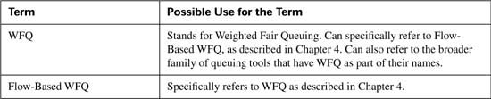
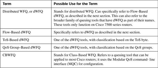
Flow-Based dWFQ classifies packets based on the flow, examining the source and destination IP address and port and the protocol type. All of the other main features of dWFQ differ slightly when compared to WFQ. Table B-15 lists several points for comparison.
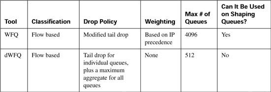
The first big difference between WFQ and dWFQ involves the tail-drop policy. dWFQ has to answer two simple questions when it determines whether to drop a packet:
![]() Has the aggregate packet limit been exceeded
Has the aggregate packet limit been exceeded
![]() Has the individual queue limit been exceeded?
Has the individual queue limit been exceeded?
If either of these questions is true (the aggregate packet limit or the individual queue limit has been exceeded), the new packet is discarded. Unlike WFQ, dWFQ cannot enqueue a packet, only to discard it later because its sequence number (SN) is larger than a new packet’s SN. dWFQ uses the terms “aggregate limit” and “individual limit” to describe the limit over all queues and the limit per queue, respectively.
Unlike WFQ, dWFQ ignores the IP precedence value when calculating the SN of a packet. In other words, dWFQ does not actually weight the packet, totally ignoring the contents of the ToS byte. In effect, all packets are weighted equally, so dWFQ always prefers lower-volume flows in comparison to higher-volume flows.
Another difference between the two is that dWFQ does allow for the maximum queue length to be changed, but the number of queues remains constant at 512.
Finally, one other difference between WFQ and dWFQ has to do with how dWFQ works internally. dWFQ uses a mechanism called a calendar queue to sort all the packets waiting in a dWFQ queue. WFQ uses a simple sorted linked list. The effect is the same—both schedulers select the packet with the lowest SN as the next packet to be forwarded to the TX Queue/TX Ring. By using a calendar queue, however, dWFQ actually performs the final scheduling function more efficiently, which is particularly useful on higher-speed interfaces. (Note that the internals of calendar queues is not important for the QoS exam; if you want to read more, however, refer to Inside Cisco IOS Software Architecture.)
dWFQ configuration, like WFQ, takes little effort. The fair-queue interface subcommand enables flow-based dWFQ on the interface. If you want to change the aggregate or individual queue limits, you use the fair-queue aggregate-limit and fair-queue individual-limit commands, respectively. You can use the same familiar show commands to examine the status of dWFQ. Tables B-16 and B-17 list the configuration commands and exec commands for Flow-Based dWFQ.
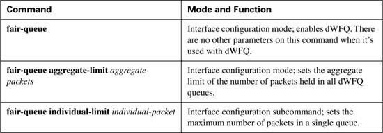

Coincidentally, in some cases, a valid configuration for WFQ can be identical to a valid configuration for dWFQ. For instance, the fair-queue subcommand is used to enable both WFQ and dWFQ on an interface. Example B-21 shows a configuration on the familiar R3, which has now been upgraded to a 7500 series router with VIP2-50 line cards:
Example B-21 dWFQ Configuration
!
interface serial 0/0/1
encapsulation ppp
description Serial interface on VIP2-50
fair-queue
In the example, CEF has been enabled globally, and the fair-queue command has been added to the serial interface. If the serial interface were not on a VIP at all, WFQ would be performed. With a VIP2-50 installed, dWFQ would be performed.
Figure B-16 summarizes the sequencing and main features of dWFQ.
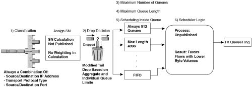
ToS-Based dWFQ uses a totally different classification method and a totally different scheduler as compared with WFQ. After reading this section, you may wonder why Cisco calls this tool WFQ at all, because it does not resemble WFQ in very many ways! ToS-Based WFQ classifies based on the 2 low-order bits in the IP Precedence field—in other words, the second and third bits of the Precedence field. It places packets into one of four queues based on these values. It does not consider the flow at all; it is a class-based tool, as opposed to a flow-based tool. Classification is based on the 2 low-order bits in the IP Precedence field, as opposed to WFQ’s flow-based classification.
Although the details are not published, ToS-Based dWFQ does use a fair-queuing scheduler, with the weighting based on the bandwidth percentages configured in each case. If only 2 queues were used, and one queue were given 75 percent of the bandwidth, and the other queue were given 25 percent, for example, internally, IOS calculates weights for the 2 queues with a ratio of 3:1. That’s why it’s called WFQ, although ToS-Based dWFQ differs significantly from WFQ. Table B-18 lists points for comparison, which are illustrated in Figure B-17.

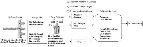
The classification function cannot be changed for ToS-Based WFQ. It always places packets into one of four queues, based on the 2 low-order bits in the IP Precedence field. In other words, precedence 0 and 4 go into Queue 0, because decimal 0 converts to 000, and decimal 4 converts to 100—so the 2 low-order bits are equal. Likewise, precedence 1 and 5 end up in Queue 1, precedence 2 and 6 in Queue 2, and precedence 3 and 7 in Queue 3.
The drop policy is just like dWFQ, using an aggregate limit and individual queue limit method to set the value.
The scheduler provides a percentage of bandwidth for each queue. Cisco does not publish the scheduler logic, but it works like WFQ, using SNs. IOS derives the weights for each queue based on the configured bandwidth percentages. Interestingly, the parameter is actually called weight, although it is interpreted as a percentage of bandwidth. The percentages default to 10 percent, 20 percent, 30 percent, and 40 percent, for Queues 0 through 3, respectively. You can configure the percentages for Queues 1 through 3, with the rest being assigned to Queue 0.
The configuration for ToS-Based dWFQ is simple. Tables B-19 and B-20 list the generic commands, and an example follows these tables.
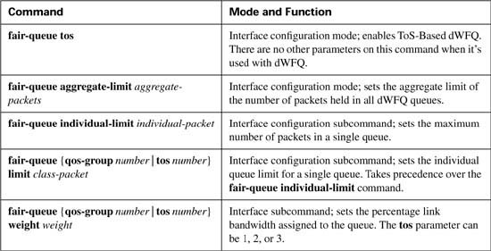
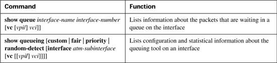
Configuring the fair-queue tos subcommand on an interface enables ToS-Based dWFQ. For this command to work, distributed CEF (dCEF) must be enabled, and the interface must really be on a VIP2-xx, where xx is 40 or higher. Example B-22 shows a sample configuration, along with changes to the bandwidth percentages given to Queues 1, 2, and 3. In this case, Queue 0 gets 39 percent of the link bandwidth, because 61 percent has been assigned using configuration commands.
QoS Group–Based dWFQ behaves almost identically to ToS-Based WFQ. The classification feature of each is similar, but with QoS Group–Based dWFQ, the classification is based on the QoS group value assigned to the packet. The QoS group is a value between 0 and 99, inclusive, which is assigned to the packet as it passes through a single router. QoS Group–Based dWFQ classifies a packet into 1 of 100 queues, numbered 0 through 99, matching the QOS group assigned to the packet. (Queue 0 is the default queue.)
The drop policy and scheduler work just like ToS-Based dWFQ as well. The bandwidth percentages can be spread among as many as 100 queues. Table B-21 lists the familiar points for comparison, this time highlighting QoS Group–Based dWFQ, and Figure B-18 depicts the general sequence of events when using QoS Group–Based dWFQ.
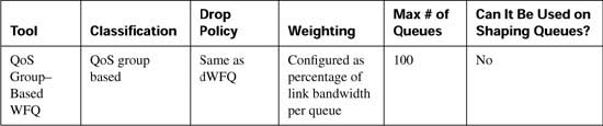
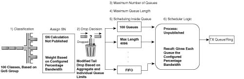
The configuration for QoS Group–Based dWFQ is simple. Tables B-22 and B-23 lists the generic commands.
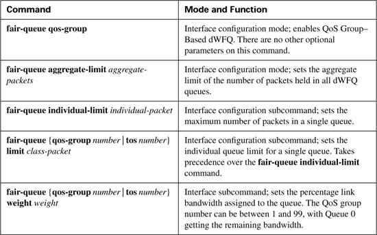
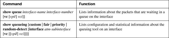
Configuring the fair-queue qos-group subcommand on an interface enables QoS Group–Based dWFQ. For this command to work, dCEF must be enabled, and the interface must really be on a VIP2-xx, where xx is 40 or higher. Example B-23 shows a sample configuration, along with changes to the bandwidth percentages given to Queues 1, 2, and 3. In this case, queue 0 gets 39 percent of the link bandwidth, because 61 percent has been assigned using configuration commands.
Example B-23 QoS Group–Based dWFQ Configuration
!
interface serial 0/0/1
encapsulation ppp
description Serial interface on VIP2-50
fair-queue qos-group
fair-queue qos-group 1 weight 30
fair-queue qos-group 2 weight 30
fair-queue qos-group 3 weight 1
Example B-23 lists the same basic parameters as Example B-13, but with QoS Group–Based dWFQ in this case. Of course, more queues could be used, with different weights (bandwidth percentages) for each queue.
Of the three dWFQ options, useful on the 7500 series routers only, dWFQ (also called Flow- Based dWFQ) is most similar to WFQ. It is flow based, uses a similar (although slightly different) drop policy, and uses the same scheduling logic. However, the other differences are significant: dWFQ does not consider the IP precedence when assigning SNs, and it only allows 512 queues.
The other two dWFQ options, ToS-Based dWFQ and QoS Group–Based dWFQ, stand out in their lack of similarity to WFQ. Neither are flow based, the number of queues is predetermined, and the scheduler assigns weights based on bandwidth percentages, which is more like CQ or CBWFQ. Like dWFQ, these two options are available only on 7500 series routers.
ToS-Based dWFQ classifies based on the 2 low-order bits in the IP Precedence field, which may require you to rethink your QoS classification and marking strategy. For instance, Cisco recommends that you mark video payload with AF41, and the least-important data with DSCP BE. The video needs high bandwidth, low delay, and low jitter. The unimportant data can get the leftover bandwidth, with no significant delay requirements. With DSCP AF41’s binary code being 100010, however, and DSCP BE being 000000, ToS-Based dWFQ would work poorly. (The low-order 2 bits of the IP Precedence field are in bold, and in both cases, the value is binary 00.) Similarly, DSCP EF traffic and DSCP AF11, AF12, and AF13 would all be placed in the same queue with ToS-Based dWFQ. Therefore, you would need to reconsider the QoS policy for marking before using this tool.
From an exam-preparation perspective, try to focus on the details of WFQ and the comparisons between the tools that Table B-24 outlines.
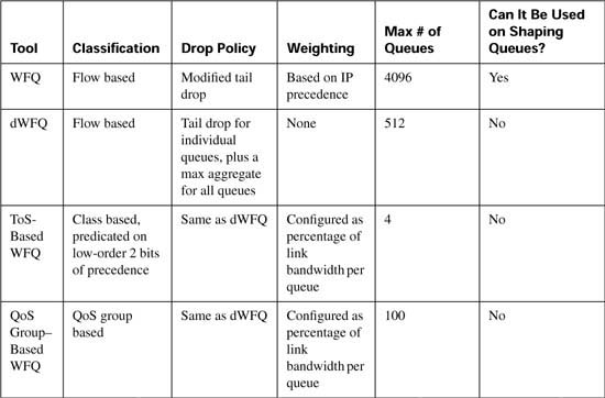
Cisco designed Modified Deficit Round-Robin (MDRR) specifically for the Gigabit Switch Router (GSR) models of Internet routers. In fact, MDRR is supported only on the GSR 12000 series routers, and the other queuing tools (WFQ, CBWFQ, PQ, CQ, and so on) are not supported on the GSRs.
Many of the features of MDRR will be familiar. Like all queuing tools, it needs to perform classification and make drop decisions, scheduling decisions, and so on. Figure B-19 depicts the major parts of the queuing puzzle of MDRR, followed by some comments about each step.
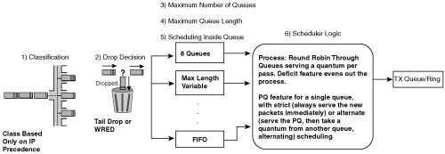
MDRR classifies packets only based on the IP Precedence field. Not surprisingly, MDRR supports eight classes, and therefore eight queues, because there are eight precedence values. The queues are numbered 0 through 7, and the precedence values (decimal) are also 0 through 7—but MDRR does map the values one to one. MDRR enables you to configure each precedence value to map to any of the queues, so more than one precedence value could map to the same queue.
Like CBWFQ, MDRR supports either tail drop or Weighted Random Early Detection (WRED) for the drop policy, per queue. Like most other tools, inside each queue, first-in, first-out (FIFO) logic is used. In addition, as expected, the most interesting part relates to the logic used by the scheduler, which is where MDRR gets its name.
MDRR schedules traffic by making a round-robin pass through the configured queues. (For the time being, assume that the optional PQ [LLQ] feature has not been configured.) MDRR removes packets from a queue, until the quantum value (QV) for that queue has been removed. The QV quantifies a number of bytes, and is used much like the byte count is used by the CQ scheduler. MDRR repeats the process for every queue, in order from 0 through 7, and then repeats this round-robin process. The end result is that each queue gets some percentage bandwidth of the link.
The CQ scheduler has a problem with trying closely to provide a particular percentage bandwidth. MDRR overcomes this same problem, but it is useful to recall an example of the problem first. Repeating an earlier example about CQ, suppose a router uses CQ on an interface, with 3 queues, with the byte counts configured to 1500, 1500, and 1500. Now suppose that all the packets in the queues are 1500 bytes. (This is not going to happen in real life, but it is useful for making the point.) CQ takes a 1500-byte packet, notices that it has met the byte count, and moves to the next queue. In effect, CQ takes one packet from each queue, and each queue gets 1/3 of the link bandwidth. Now suppose that Queue 3 has been configured to send 1501 bytes per queue service, and all the packets in all queues are still 1500 bytes long. CQ takes 1 packet from Queue 1, 1 from Queue 2, and then 2 packets from Queue 3! CQ does not fragment the packet. In effect, Queue 3 sends 2 packets for every 1 packet sent from Queues 1 and 2, effectively giving 25 percent of the bandwidth each to Queues 1 and 2, and 50 percent of the link bandwidth to Queue 3.
MDRR deals with this problem by treating any “extra” bytes sent during a cycle as a “deficit.” Next time around through the queues, the number of “extra” bytes sent by MDRR is subtracted from the QV. In Figure B-20, MDRR is using only two queues, with QVs of 1500 and 3000, respectively, and with all packets at 1000 bytes in length.
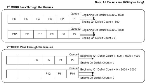
First, some extra information on how to interpret the figure may help. The figure shows the action during the first round-robin pass in the top half of the figure, and the action during the second pass in the lower half of the figure. The example begins with six packets (labeled P1 through P6) in Queue 1, and six packets (labeled P7 through P12) in Queue 2. Each arrowed line, attached to the right sides of the queues, and pointing to the right, represents the choice by MDRR to send a single packet.
When a queue first fills, the queue’s deficit counter is set to the QV for that queue, which is 1500 for Queue 1, and 3000 for Queue 2. In the figure, MDRR begins by taking 1 packet from Queue 1, decrementing the DC to 500, and deciding that the DC has not been decremented to 0 (or less).
MDRR takes a second packet from Queue 1, decrementing the DC to –500. MDRR then moves on to Queue 2, taking three packets, after which the DC for Queue 2 has decremented to 0.
That concludes the first pass through the queues. MDRR has taken 2000 bytes from Queue 1, and 3000 from Queue 2, giving the queues 40 percent and 60 percent of link bandwidth, respectively.
In the second round-robin pass, shown in the lower half of the figure, the process begins by MDRR adding the QV for each queue to the DC for each queue. Queue 1’s DC becomes 1500 + –500, or 1000, to begin the second pass. During this pass, MDRR takes P3 from Queue 1, decrements DC to 0, and then moves on to Queue 2. After taking three more packets from Queue 3, decrementing Queue 2’s DC to 0, MDRR completes the second pass. Over these two round-robin passes, MDRR has taken 3000 bytes from Queue 1, and 6000 from Queue 2—which is the same ratio as the ratio between the QVs.
With the deficit feature of MDRR, over time each queue receives a guaranteed bandwidth based on the following formula:
![]()
Note For additional examples of the operation of the MDRR deficit feature, refer to http://www.cisco.com/warp/public/63/toc_18841.html. Alternatively, you can go to www.cisco.com and search for “Understanding and Configuring MDRR and WRED on the Cisco 12000 Series Internet Router.”
MDRR also allows one queue to be used as a PQ, but with two variations on how the PQ is scheduled. One scheduling option, called strict scheduling, acts just like PQ’s treatment of the High queue, which is also how Low Latency Queuing (LLQ) and IP RTP Priority scheduling works. Whenever the scheduler decides to remove another packet from any queue, it first checks the strict PQ, and takes a packet if one is in the queue. With strict treatment, MDRR does not need to assign a QV to the low-latency queue, because there is no concept of taking a QV of bytes per pass through the queue—the low-latency queue gets strict service whenever it needs it.
MDRR offers a less strict algorithm for servicing the low-latency queue called alternate service. With alternate service, the low-latency queue is assigned a QV, just like the other queues. MDRR takes QV bytes from the low-latency queue, and then take bytes from a non-low-latency queue. MDRR then goes back to the low-latency queue, taking QV bytes, and then to another queue. If Queues 0 through 2 are Normal queues, and Queue 7 is the low-latency queue, for instance, MDRR serves the queues in this order: 7, 0, 7, 1, 7, 2, and repeats this sequence. Because the low-latency queue gets serviced on every alternate attempt, it can get a disproportionate amount of bandwidth. However, with alternate service, MDRR does prevent the low- latency queue from taking over the link.
Strict and alternate priority affect delay and jitter differently. With alternate priority, packets experience longer delay and more jitter, as compared with strict scheduling. Alternate priority gives the other queues a little more service, however, which improves their performance.
Table B-25 summarizes some of the key features of MDRR.
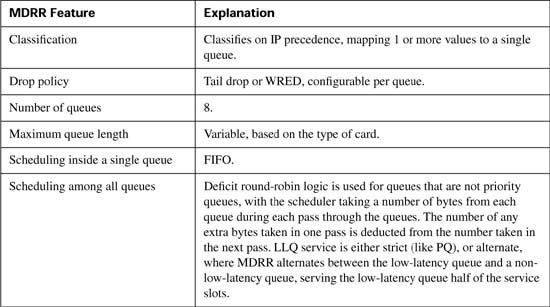
MDRR configuration requires you to understand GSR architecture to a small degree. MDRR configuration also introduces some new terminology. Table B-26 lists the configuration commands related to MDRR, and following the tables is an explanation of the new terminology, the formula used to calculate the QV per queue, and an explanation of the flow of the configuration commands.
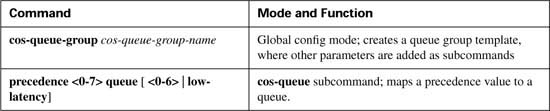
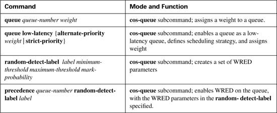
After you understand the basic concepts, you just need to understand a few facts about how the configuration commands work before being able to configure basic MDRR. First, the low- latency queue is always Queue 7, and instead of being referred to as Queue 7, the low-latency queue is referred to with the low-latency keyword. The next thing to note is that the QoS configuration details are configured as subcommands of the cos-queue-group command. In other words, the classification details, choosing QVs by using the weight keyword, and selecting strict or alternate LLQ scheduling, are configured as subcommands of the cos-queue- group command. MDRR configuration does not enable you to specify the QV for each queue, but rather you configure a value called weight. The QV is then calculated from the weight using the following formula:
Here, MTU is the maximum transmission unit configured for the interface. Weight values can be configured between 1 and 2048, but Cisco recommends using low values—in fact, for the lowest-weight queue, use a value of 1.
Finally, like LAN switches, GSR routers benefit from having both input and output queuing. MDRR can be applied to an interface for input packets using the rx-cos command, and for output packets using the tx-cos command.
The following criteria is used in the upcoming example configuration:
![]() Precedence 0 and 1 are placed in Queue 0, with a weight of 1.
Precedence 0 and 1 are placed in Queue 0, with a weight of 1.
![]() Precedence 5 is placed in the low-latency queue, with strict priority.
Precedence 5 is placed in the low-latency queue, with strict priority.
![]() All other precedence values are placed in Queue 1, with a weight of 3.
All other precedence values are placed in Queue 1, with a weight of 3.
![]() WRED is used on Queues 0 and 1, with default WRED parameters.
WRED is used on Queues 0 and 1, with default WRED parameters.
![]() The MDRR configuration is used for packets entering interface pos (Packet over SONET) 3/0, and for packets exiting pos 3/1.
The MDRR configuration is used for packets entering interface pos (Packet over SONET) 3/0, and for packets exiting pos 3/1.
Example B-24 shows the configuration and show commands.
Example B-24 MDRR: VoIP in High Queue, All Else in Normal Queue
Rx-cos my-sample
Interface pos 3/1
Tx-cos my-sample
!
cos-queue-group my-sample
precedence 0 queue 0
precedence 0 random-detect-label 0
precedence 1 queue 0
precedence 1 random-detect-label 0
precedence 2 queue 1
precedence 2 random-detect-label 0
precedence 3 queue 1
precedence 3 random-detect-label 0
precedence 4 queue 1
precedence 4 random-detect-label 0
precedence 5 queue low-latency
precedence 6 queue 1
precedence 6 random-detect-label 0
precedence 7 queue 1
precedence 7 random-detect-label 0
!
precedence 0 random-detect-label 0
!
queue 0 1
queue 1 3
queue low-latency strict
!
random-detect-label 0
Most of the commands in the sample are configuration subcommands under the cos-queue- group my-sample command. For instance, the precedence 0 queue 0 command maps precedence 0 packets to Queue 0; a similar command maps the appropriate precedence values to queues, as stated in the policy before the example. Similarly, WRED parameters apply per precedence, so the precedence 0 random-detect-label 0 command links precedence 0 packets to a set of WRED parameters with a WRED label of 0. At the end of the example, the random- detect-label 0 command creates a WRED label 0, with no specific parameters—even if you want to take default WRED parameters, you still need to create the label, and refer to it with a command such as precedence 0 random-detect-label 0 to enable WRED for those packets.
The weights are configured with the queue command seen toward the end of the configuration. The queue 0 1 command assigns a weight of 1 to Queue 0, and the queue 1 3 command assigns a weight of 3 to Queue 1. The queue low-latency strict command defines that Queue 7, the low-latency queue, should use strict scheduling.
Finally, at the top of the configuration, the rx-cos my-sample command enables cos-queue-list my-sample for packets entering interface pos 3/0. Similarly, the tx-cos my-sample interface subcommand enables MDRR for packets exiting pos 3/1.
MDRR provides queuing services on GSR 12000 series routers. It assigns a percentage bandwidth through the use of the weight keyword, with the percentages being much more exact than CQ through the deficit feature of the MDRR scheduler. MDRR allows two options for treatment of the low-latency queue, strict and alternate, which gives the engineer more flexibility in how to deal with delay- and jitter-sensitive traffic.
The classification feature of MDRR only supports IP precedence, which can be seen as a negative. Because most networks deploy GSRs in the core of the network, however, a good QoS design, with classification and marking at the edge of the network, can work very well with the precedence-based classification of MDRR.
This section covers GTS, DTS, FRTS, and CAR (as a policing tool).
GTS performs traffic shaping using the same logic and features discussed in the introductory section of this chapter. It can be enabled on a large variety of interfaces. It can also adapt the rate based on BECN signals, and reflect BECNs on a VC after receiving a FECN. It supports a single queuing tool for the shaping queues: Weighted Fair Queuing (WFQ). It can also classify traffic, performing shaping on a subset of the traffic on an interface by classifying packets based on access control lists (ACLs).
The only feature of GTS not already covered to some depth, other than configuration, is the concept of shaping a subset of the traffic on an interface or subinterface. GTS can classify traffic with an ACL; traffic permitted by the ACL is shaped based on the parameters specified on the same command. For instance, you could shape all FTP traffic to 32 kbps, and web traffic to 64 kbps.
Other than the material already covered, the only other thing really left to think about with GTS is how to configure it. Tables B-27 and B-28 list the configuration and show commands pertinent to GTS.
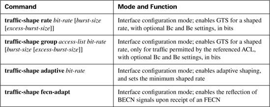
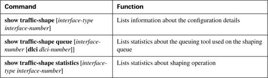
The examples in this section use a familiar network diagram, as shown in Figure B-21. The configuration shows R3, with a 128-kbps access rate, and a 64-kbps Frame Relay VC connecting to R1. Traffic from R3 to R1 is Shaped using the following criteria:
![]() Shape all traffic at a 64 kbps rate.
Shape all traffic at a 64 kbps rate.
![]() Use the default setting for Tc.
Use the default setting for Tc.
![]() Enable the configuration per VC.
Enable the configuration per VC.
![]() Use WFQ on the physical interface output queues.
Use WFQ on the physical interface output queues.
![]() Use WFQ on the shaping queues (only choice available).
Use WFQ on the shaping queues (only choice available).
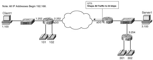
In each example, the client downloads one web page, which has two frames inside the page. The web page uses two separate TCP connections to download two separate large JPG files that are shown in each of the two frames inside the browser window. The client also downloads a file using FTP. Additionally, a VoIP call is placed between extension 302 and 102. Example B-25 shows the configuration and some sample show commands.
Example B-25 CB Shaping on R3, 64-kbps Shape Rate
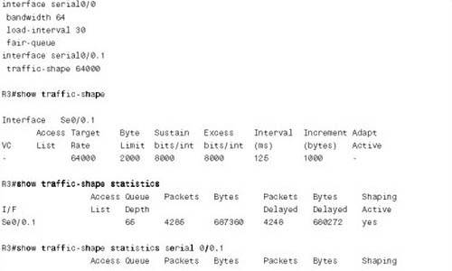
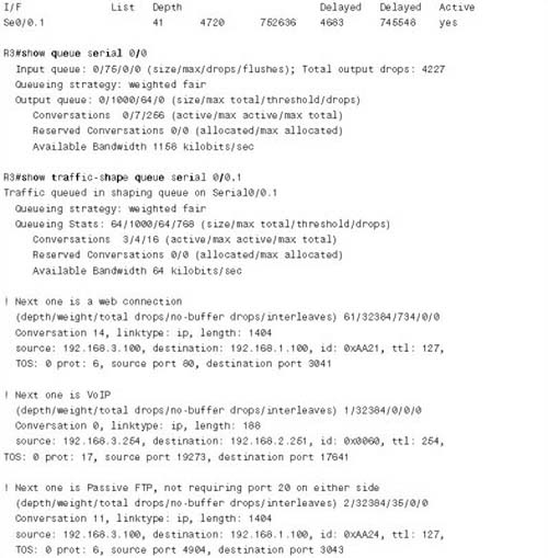
The configuration itself is rather simple. You can configure GTS on the subinterface, or on the main interface in this case, because only one VC runs out of the interface. Because most installations tend to enable GTS on subinterfaces, the traffic-shape rate 64000 command was added to interface s0/0.1 to enable GTS for a shaping rate of 64 kbps. GTS only allows WFQ on the shaping queues, so no other configuration command is needed to enable WFQ. The fair- queue command on the physical interface enables WFQ just for the interface output queues.
Three show commands list information about GTS. First, immediately after the configuration, the show traffic-shape command lists basic configuration information, and the derived values for Bc and Be of 8000 bits each. Bc was derived by IOS using the formula Bc = Tc * CIR, which is just a variation on the Tc = Bc/CIR formula. The Tc value defaults to 125 ms, but interestingly, GTS can use different default Tc values, based on the configuration settings you use.
GTS uses WFQ for the shaping queues; the next command in the example, show traffic-shape queue, supplies the same output that the show queue command does for WFQ on an interface.
Finally, the show traffic-shape statistics command lists basic statistics about GTS. The last column of output is particularly interesting, because it tells you whether shaping is currently active. IOS does not need to shape all the time, so this column just lists the current state when the command was issued. Shaping activates for three reasons:
![]() If adaptive shaping is currently reacting to BECNs by lowering the shaped rate
If adaptive shaping is currently reacting to BECNs by lowering the shaped rate
![]() If Bc and Be have been exceeded, causing packets to be delayed
If Bc and Be have been exceeded, causing packets to be delayed
![]() If Frame Relay fragmentation is enabled
If Frame Relay fragmentation is enabled
Queuing occurs on the physical interface when the traffic load exceeds the interface clock rate, and shaping queues form when the traffic load exceeds the shaping rate. In this case, with a single VC, shaped at 64 kbps, and a 128-kbps clock rate on the physical interface, no queues should form on the physical interface. The offered load on the physical link should not exceed 64 kbps, because that is how much traffic the GTS will allow to pass through the only subinterface in the example. The output of the show queue and show traffic-shape queue commands in the example support these facts. The show queue command lists information about WFQ on the physical interface; it does not list any flows, because no congestion is occurring there. However, the show traffic-shape queue command lists information about WFQ’s performance with the shaping queues. In this case, it lists information about a VoIP call, and one FTP download.
This particular example reminds us of the importance of the queuing methods supported by the shaping tool. Because GTS only supports WFQ in conjunction with shaping, there is no low- latency option, such as LLQ. The VoIP call in this particular example had a completely unusable quality level.
A second GTS configuration example is shown next. For the second configuration, imagine that the Frame Relay provider actually polices the VC from R3 to R1 at 96 kbps. You engineer the network to support a single G.729 VoIP call, which takes about 28 kbps. You decide that you want to be very careful about packet drops, latency, and jitter for this voice traffic, so you decide to shape all traffic except voice. To avoid drops inside the cloud, you shape the rest of the traffic to a rate of 64 kbps (so that the combined single VoIP call, and the shaped rate of 64 kbps, do not exceed the policing rate in the Frame Relay network). The next example shows the configuration, and the criteria for the configuration is as follows:
![]() Shape non-VoIP traffic at 64 kbps.
Shape non-VoIP traffic at 64 kbps.
![]() Choose values so Tc is 50 ms.
Choose values so Tc is 50 ms.
![]() Enable the configuration on the subinterface.
Enable the configuration on the subinterface.
![]() Use WFQ on the physical interface output queues.
Use WFQ on the physical interface output queues.
![]() Use WFQ on the shaping queues (the only choice available).
Use WFQ on the shaping queues (the only choice available).
The traffic generated for this second example is the same type of traffic generated for the first—a single VoIP call, one web page downloaded with two frames inside the page (causing two TCP connections), and an FTP get. Example B-26 shows the configuration and some sample show commands.
Example B-26 GTS on R3, 64 kbps for Non-Voice Traffic, Tc = 50 ms
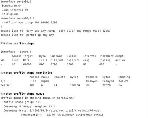
Available Bandwidth 64 kilobits/sec
(depth/weight/total drops/no-buffer drops/interleaves) 3/32384/0/0/0
Conversation 11, linktype: ip, length: 1404
source: 192.168.3.100, destination: 192.168.1.100, id: 0xB077, ttl: 127,
TOS: 0 prot: 6, source port 4904, destination port 3043
R3#show access-lists
Extended IP access list 101
deny udp any range 16384 32767 any range 16384 32767 (18638 matches)
permit ip any any (1257 matches)
The configuration enables GTS by using the traffic-shape group 101 64000 3200 command. This command refers to ACL 101, which permits all traffic except VoIP traffic, implying that shaping occurs for all traffic except VoIP. The shaped rate of 64 kbps implies that the traffic permitted by the ACL will be shaped to 64 kbps. Also note that, according to the traffic-shape command, the Bc value was set to 3200, which should give a Tc of 3200/64,000, or 50 ms. The show traffic-shape command confirms the calculated Tc value, listing it as 50 ms. Also note that the Be value was set to 3200, because GTS defaults Be to be equal to Bc.
Note All IOS shapers use bits as the unit when setting Bc and Be; both policers use bytes as the unit.
The show access-lists command lists the number of packets permitted and denied by ACL 101. Because ACL 101 is used for matching by GTS, this also tells us how many packets were shaped by GTS, and how many were not.
GTS supports several useful traffic-shaping features. It can be used on many types of interfaces, and it can shape a subset of the traffic by referencing ACLs. It can also adapt to BECNs, and reflect FECNs. However, GTS does have several drawbacks. It only supports WFQ in the shaping queues, and it cannot support FRF.12 fragmentation on Frame Relay subinterfaces. Table B-29 summaries the key points for comparison between the various traffic-shaping tools, and lists whether GTS supports each.
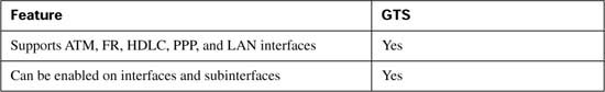
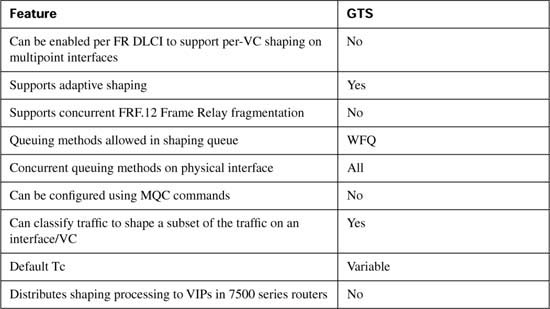
DTS shapes traffic identically to CB shaping, but with processing distributed to VIPs in a 7500 series router. In fact, DTS and CB shaping configurations are very similar, but with a few extra requirements. Distributed CEF must be configured for the interfaces on which DTS should operate. DTS also has a few idiosyncrasies that are not mentioned in either of the QoS courses, so they are unlikely to be on the exam.
Note If you want to read further about DTS, look for the “Cisco AVVID Enterprise Quality of Service Infrastructure Quality of Service Design” document at www.cisco.com/warp/customer/771/srnd/qos_srnd.pdf. On pages 4 through 18 of that document, the text outlines some of the unique requirements for DTS that are beyond the scope of the QoS exams, but important in real networks. This document is a very good reference for QoS design recommendations across all QoS functions and Cisco product lines.
To configure DTS, just complete these listed tasks: