Chapter 12

Multivariate Smoothing

12.1 Predictor–Response Data

Multivariate predictor–response smoothing methods fit smooth surfaces to observations (x_i, y_i), where x_i is a vector of p predictors and y_i is the corresponding response value. The y₁, . . ., y_n values are viewed as observations of the random variables Y₁, . . ., Y_n, where the distribution of Y_i depends on the ith vector of predictor variables.

Many of the bivariate smoothing methods discussed in Chapter 11 can be generalized to the case of several predictors. Running lines can be replaced by running planes. Univariate kernels can be replaced by multivariate kernels. One generalization of spline smoothing is thin plate splines [280, 451]. In addition to the significant complexities of actually implementing some of these approaches, there is a fundamental change in the nature of the smoothing problem when using more than one predictor.

The curse of dimensionality is that high-dimensional space is vast, and points have few near neighbors. This same problem was discussed in Section 10.4.1 as it applied to multivariate density estimation. Consider a unit sphere in p dimensions with volume π^p/2/Γ(p/2 + 1). Suppose that several p-dimensional predictor points are distributed uniformly within the ball of radius 4. In one dimension, 25% of predictors are expected within the unit ball; hence unit balls might be reasonable neighborhoods for smoothing. Table 12.1 shows that this proportion vanishes rapidly as p increases. In order to retain 25% of points in a neighborhood when the full set of points lies in a ball of radius 4, the neighborhood ball would need to have radius 3.73 if p = 20. Thus, the concept of local neighborhoods is effectively lost.

Table 12.1 Ratio of volume of unit sphere in p dimensions to volume of sphere with radius 4.

	Ratio
1	0.25
2	0.063
3	0.016
4	0.0039
5	0.00098
10	9.5 × 10−7
20	9.1 × 10−13
100	6.2 × 10−61

The curse of dimensionality raises concerns about the effectiveness of smoothers for multivariate data. Effective local averaging will require a large number of points in each neighborhood, but to find such points, the neighborhoods must stretch over most of predictor space. A variety of effective multivariate surface smoothing methods are described in [322, 323, 573].

There is a rich set of smoothing methods developed for geostatistics and spatial statistics that are suitable for two and three dimensions. In particular, kriging methods offer a more principled foundation for inference than many of the generic smoothers considered here. We do not consider such methods further, but refer readers to books on spatial statistics such as [128, 291].

12.1.1 Additive Models

Simple linear regression is based on the model E{Y|x} = β₀ + β₁x. Nonparametric smoothing of bivariate predictor–response data generalizes this to E{Y|x} = s(x) for a smooth function s. Now we seek to extend the analogy to the case with p predictors. Multiple regression uses the model where x = (x₁, . . ., x_p)^T. The generalization for smoothing is the additive model

(12.1)

where s_k is a smooth function of the kth predictor variable. Thus, the overall model is composed of univariate effects whose influence on the mean response is additive.

Fitting such a model relies on the relationship

(12.2)

where x_k is the kth component in x. Suppose that we wished to estimate s_k at , and that many replicate values of the kth predictor were observed at exactly this . Suppose further that all the s_j (j ≠ k) were known except s_k. Then the expected value on the right side of (12.2) could be estimated as the mean of the values of Y_i − α − ∑ _j≠ks_j(x_ij) corresponding to indices i for which the ith observation of the kth predictor satisfies . For actual data, however, there will likely be no such replicates. This problem can be overcome by smoothing: The average is taken over points whose kth coordinate is in a neighborhood of . A second problem—that none of the s_j are actually known—is overcome by iteratively cycling through smoothing steps based on isolations like (12.2) updating s_k using the best current guesses for all s_j for j ≠ k.

The iterative strategy is called the backfitting algorithm. Let Y = (Y₁, . . ., Y_n)^T, and for each k, let denote the vector of estimated values of s_k(x_ik) at iteration t for i = 1, . . ., n. These n-vectors of estimated smooths at each observation are updated as follows:

1. Let be the n-vector . Some other generalized average of the response values may replace the sample mean . Let t = 0, where t indexes the iteration number.

2. Let represent initial guesses for coordinatewise smooths evaluated at the observed data. A reasonable initial guess is to let for k = 1, . . ., p, where the are the linear regression coefficients found when Y is regressed on the predictors.

3. For k = 1, . . ., p in turn, let

(12.3)

where

(12.4)

and smooth_k(r_k) denotes the vector obtained by smoothing the elements of r_k against the kth coordinate values of predictors, namely x_1k, . . ., x_nk, and evaluating the smooth at each x_ik. The smoothing technique used for the kth smooth may vary with k.

4. Increment t and go to step 3.

The algorithm can be stopped when none of the change very much—perhaps when

is very small.

To understand why this algorithm works, recall the Gauss–Seidel algorithm for solving a linear system of the form Az = b for z given a matrix A and a vector b of known constants (see Section 2.2.5). The Gauss–Seidel procedure is initialized with starting value z₀. Then each component of z is solved for in turn, given the current values for the other components. This process is iterated until convergence.

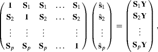
Suppose only linear smoothers are used to fit an additive model, and let S_k be the n × n smoothing matrix for the kth component smoother. Then the backfitting algorithm solves the set of equations given by . Writing this set of equations in matrix form yields

(12.5)

which is of the form Az = b where . Note that b = ΛY where Λ is a block-diagonal matrix with the individual S_k matrices along the diagonal. Since the backfitting algorithm sequentially updates each vector as a single block, it is more formally a block Gauss–Seidel algorithm. The iterative backfitting algorithm is preferred because it is faster than the direct approach of inverting A.

We now turn to the question of convergence of the backfitting algorithm and the uniqueness of the solution. Here, it helps to revisit the analogy to multiple regression. Let D denote the n × p design matrix whose ith row is so D = (x₁, . . ., x_n)^T. Consider solving the multiple regression normal equations D^TDβ = D^TY for β. The elements of β are not uniquely determined if any predictors are linearly dependent, or equivalently, if the columns of D^TD are linearly dependent. In that case, there would exist a vector γ such that D^TDγ = 0. Thus, if were a solution to the normal equations, would also be a solution for any c.

Analogously, the backfitting estimating equations will not have a unique solution if there exists any γ such that Aγ = 0. Let be the space spanned by vectors that pass through the kth smoother unchanged. If these spaces are linearly dependent, then there exist such that . In this case, Aγ = 0, where γ = (γ₁, γ₂, . . ., γ_p)^T, and therefore there is not a unique solution (see Problem 12.1).

A more complete discussion of these issues is provided by Hastie and Tibshirani [322], from which the following result is derived. Let the p smoothers be linear and each S_k be symmetric with eigenvalues in [0, 1]. Then Aγ = 0 if and only if there exist linearly dependent that pass through the kth smoother unchanged. In this case, there are many solutions to , and backfitting converges to one of them, depending on the starting values. Otherwise, backfitting converges to the unique solution.

The flexibility of the additive model is further enhanced by allowing the additive components of the model to be multivariate and by allowing different smoothing methods for different components. For example, suppose there are seven predictors, x₁, . . ., x₇, where x₁ is a discrete variable with levels 1, . . ., c. Then an additive model to estimate E{Y|x} might be fitted by backfitting:

(12.6)

where the permit a separate additive effect for each level of X₁, is a spline smooth over x₂, is a cubic polynomial regression on x₃, is a recursively partitioned regression tree from Section 12.1.4, and is a bivariate kernel smooth. Grouping several predictors in this way provides coarser blocks in the blockwise implementation of the Gauss–Seidel algorithm.

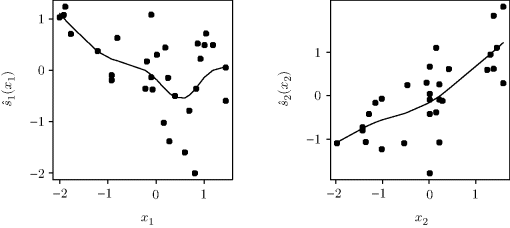
Example 12.1 (Norwegian Paper) We consider some data from a paper plant in Halden, Norway [9]. The response is a measure of imperfections in the paper, and there are two predictors. (Our Y, x₁, and x₂ correspond to 16 − Y₅, X₁, and X₃, respectively, in the author's original notation.) The left panel of Figure 12.1 shows the response surface fitted by an ordinary linear model with no interaction. The right panel shows an additive model fitted to the same data. The estimated are shown in Figure 12.2. Clearly x₁ has a nonlinear effect on the response; in this sense the additive model is an improvement over the linear regression fit.

Figure 12.1 Linear (left) and additive (right) models fitted to the Norwegian paper data in Example 12.1.

Figure 12.2 The smooths fitted with an additive model for the Norwegian paper data in Example 12.1. The points are partial residuals as given on the right-hand side of (12.3), namely, plus the overall residual from the final smooth.

12.1.2 Generalized Additive Models

Linear regression models can be generalized in several ways. Above, we have replaced linear predictors with smooth nonlinear functions. A different way to generalize linear regression is in the direction of generalized linear models [446].

Suppose that Y|x has a distribution in the exponential family. Let μ = E{Y|x}. A generalized linear model assumes that some function of μ is a linear function of the predictors. In other words, the model is , where g is the link function. For example, the identity link g(μ) = μ is used to model a Gaussian distributed response, g(μ) = log μ is used for log-linear models, and g(μ) = log {μ/(1 − μ)} is one link used to model Bernoulli data.

Generalized additive models (GAMs) extend the additive models of Section 12.1.1 in a manner analogous to how generalized linear models extend linear models. For response data in an exponential family, a link function g is chosen, and the model is

(12.7)

where s_k is a smooth function of the kth predictor. The right-hand side of (12.7) is denoted η and is called the additive predictor. GAMs provide the scope and diversity of generalized linear models, with the additional flexibility of nonlinear smooth effects in the additive predictor.

For generalized linear models, estimation of μ = E{Y|x} proceeds via iteratively reweighted least squares. Roughly, the algorithm proceeds by alternating between (i) constructing adjusted response values and corresponding weights, and (ii) fitting a weighted linear regression of the adjusted response on the predictors. These steps are repeated until the fit has converged.

Specifically, we described in Section 2.2.1.1 how the iteratively reweighted least squares approach for fitting generalized linear models in exponential families is in fact the Fisher scoring approach. The Fisher scoring method is ultimately motivated by a linearization of the score function that yields an updating equation for estimating the parameters. The update is achieved by weighted linear regression. Adjusted responses and weights are defined as in (2.41). The updated parameter vector consists of the coefficients resulting from a weighted linear least squares regression for the adjusted responses.

For fitting a GAM, weighted linear regression is replaced by weighted smoothing. The resulting procedure, called local scoring, is described below. First, let μ_i be the mean response for observation i, so μ_i = E{Y_i|x_i} = g⁻¹(η_i), where η_i is called the ith value of the additive predictor; and let V(μ_i) be the variance function, namely, var {Y_i|x_i} expressed as a function of μ_i. The algorithm proceeds as follows:

1. Initialize the algorithm at t = 0. Set and for k = 1, . . ., p. This also initializes the additive predictor values and the fitted values corresponding to each observation.

2. For i = 1, . . ., n, construct adjusted response values

(12.8)

3. For i = 1, . . ., n, construct the corresponding weights

(12.9)

4. Use a weighted version of the backfitting algorithm from Section 12.1.1 to estimate new additive predictors, . In this step, a weighted additive model of the form (12.7) is fitted to the adjusted response values with weights , yielding for i = 1, . . ., n and k = 1, . . ., p. This step, described further below, also allows calculation of new and .

5. Compute a convergence criterion such as

(12.10)

and stop when it is small. Otherwise, go to step 2.

To revert to a standard generalized linear model, the only necessary change would be to replace the smoothing in step 4 with weighted least squares.

The fitting of a weighted additive model in step 4 requires weighted smoothing methods. For linear smoothers, one way to introduce weights is to multiply the elements in the ith column of S by for each i, and then standardize each row so it sums to 1. There are other, more natural approaches to weighting some linear smoothers (e.g., splines) and nonlinear smoothers. Further details about weighted smooths and local scoring are provided in [322, 574].

As with additive models, the linear predictor in GAMs need not consist solely of univariate smooths of the same type. The ideas in Section 12.1.1 regarding more general and flexible model building apply here too.

Example 12.2 (Drug Abuse) The website for this book provides data on 575 patients receiving residential treatment for drug abuse [336]. The response variable is binary, with Y = 1 for a patient who remained drug-free for one year and Y = 0 otherwise. We will examine two predictors: number of prior drug treatments (x₁) and age of patient (x₂). A simple generalized additive model is given by Y_i|x_i ~ Bernoulli(π_i) with

(12.11)

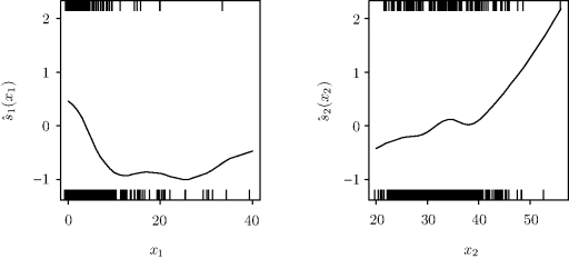
Spline smoothing was used in step 4 of the fitting algorithm. Figure 12.3 shows the fitted response surface graphed on the probability scale. Figure 12.4 shows the fitted smooths on the logit scale. The raw response data are shown by hash marks along the bottom (y_i = 0) and top (y_i = 1) of each panel.

Figure 12.3 The fit of a generalized additive model to the drug abuse data described in Example 12.2. The vertical axis corresponds to the predicted probability of remaining drug free for one year.

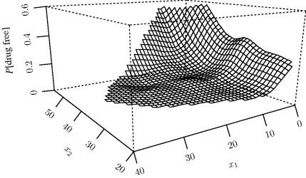
Figure 12.4 The smooth functions fitted with a generalized additive model for the drug-abuse data in Example 12.2. The raw response data are shown via the hash marks along the bottom (y_i = 0) and top (y_i = 1) of each panel at the locations observed for the corresponding predictor variable.

12.1.3 Other Methods Related to Additive Models

Generalized additive models are not the only way to extend the additive model. Several other methods transform the predictors or response in an effort to provide a more effective model for the data. We describe four such approaches below.

12.1.3.1 Projection Pursuit Regression

Additive models produce fits composed of p additive surfaces, each of which has a nonlinear profile along one coordinate axis while staying constant in orthogonal directions. This aids interpretation of the model because each nonlinear smooth reflects the additive effect of one predictor. However, it also limits the ability to fit more general surfaces and interaction effects that are not additively attributable to a single predictor. Projection pursuit regression eliminates this constraint by allowing effects to be smooth functions of univariate linear projections of the predictors [209, 380].

Specifically, these models take the form

(12.12)

where each term is a one-dimensional projection of the predictor vector x = (x₁, . . ., x_p)^T. Thus each s_k has a profile determined by s_k along a_k and is constant in all orthogonal directions. In the projection pursuit approach, the smooths s_k and the projection vectors a_k are estimated for k = 1, . . ., M to obtain the optimal fit. For sufficiently large M, the expression in (12.12) can approximate an arbitrary continuous function of the predictors [161, 380].

To fit such a model, the number of projections, M, must be chosen. When M > 1, the model contains several smooth functions of different linear combinations . The results may therefore be very difficult to interpret, notwithstanding the model's usefulness for prediction. Choosing M is a model selection problem akin to choosing the terms in a multiple regression model, and analogous reasoning should apply. One approach would be to fit a model with small M first, then repeatedly add the most effective next term and refit. A sequence of models is thus produced, until no further additional term substantially improves the fit.

For a given M, fitting (12.12) can be carried out using the following algorithm:

1. Begin with m = 0 by setting .

2. Increment m. Define the current working residual for observation i as

(12.13)

for i = 1, . . ., n, where the summation vanishes if m = 1. These current residuals will be used to fit the mth projection.

3. For any p-vector a and smoother s_m, define the goodness-of-fit measure

4. For a chosen type of smoother, maximize Q(a) with respect to a. This provides a_m and . If m = M, stop; otherwise go to step 2.

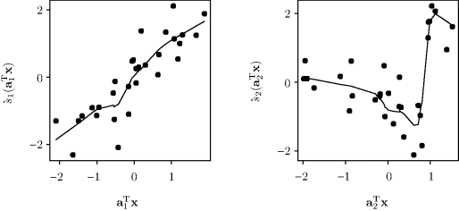
Example 12.3 (Norwegian Paper, Continued) We return to the Norwegian paper data of Example 12.1. Figure 12.5 shows the response surface fitted with projection pursuit regression for M = 2. A supersmoother (Section 11.4.2) was used for each projection. The fitted surface exhibits some interaction between the predictors that is not captured by either model shown in Figure 12.1. An additive model was not wholly appropriate for these predictors. The heavy lines in Figure 12.5 show the two linear directions onto which the bivariate predictor data were projected. The first projection direction, labeled , is far from being parallel to either coordinate axis. This allows a better fit of the interaction between the two predictors. The second projection very nearly contributes an additive effect of x₁. To further understand the fitted surface, we can examine the individual , which are shown in Figure 12.6. These effects along the selected directions provide a more general fit than either the regression or the additive model.

Figure 12.5 Projection pursuit regression surface fitted to the Norwegian paper data for M = 2, as described in Example 12.3.

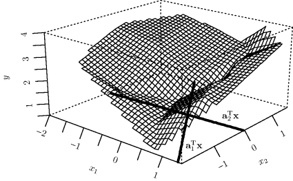
Figure 12.6 The smooth functions fitted with a projection pursuit regression model for the Norwegian paper data. The current residuals, namely the component-fitted smooth plus the overall residual, shown as dots, are plotted against each projection for k = 1, 2.

In addition to predictor–response smoothing, the ideas of projection pursuit have been applied in many other areas, including smoothing for multivariate response data [9] and density estimation [205]. Another approach, known as multivariate adaptive regression splines (MARS), has links to projection pursuit regression, spline smoothing (Section 11.2.5), and regression trees (Section 12.1.4.1) [207]. MARS may perform very well for some datasets, but recent simulations have shown less promising results for high-dimensional data [21].

12.1.3.2 Neural Networks

Neural networks are a nonlinear modeling method for either continuous or discrete responses, producing a regression or classification model [50, 51, 323, 540]. For a continuous response Y and predictors x, one type of neural network model, called the feed-forward network, can be written as

(12.15)

where β₀, β_m, α_m, and γ_m for m = 1, . . ., M are estimated from the data. We can think of the for m = 1, . . ., M as being analogous to a set of basis functions for the predictor space. These , whose values are not directly observed, constitute a hidden layer, in neural net terminology. Usually the analyst chooses M in advance, but data-driven selection is also possible. In (12.15), the form of the activation function, f, is usually chosen to be logistic, namely f(z) = 1/[1 + exp { − z}]. We use g as a link function. Parameters are estimated by minimizing the squared error, typically via gradient-based optimization.

Neural networks are related to projection pursuit regression where s_k in (12.12) is replaced by a parametric function f in (12.15), such as the logistic function. Many enhancements to the simple neural network model given above are possible, such as the inclusion of an additional hidden layer using a different activation function, say h. This layer is composed of evaluations of h at a number of linear combinations of the for m = 1, . . ., M, roughly serving as a basis for the first hidden layer. Neural networks are very popular in some fields, and a large number of software packages for fitting these models are available.

12.1.3.3 Alternating Conditional Expectations

The alternating conditional expectations (ACE) procedure fits models of the form

(12.16)

where g is a smooth function of the response [64]. Unlike most other methods in this chapter, ACE treats the predictors as observations of a random variable X, and model fitting is driven by consideration of the joint distribution of Y and X. Specifically, the idea of ACE is to estimate g and s_k for k = 1, . . ., p such that the magnitude of the correlation between g(Y) and is maximized subject to the constraint that var {g(Y)} = 1. The constant α does not affect this correlation, so it can be ignored.

To fit the ACE model, the following iterative algorithm can be used:

1. Initialize the algorithm by letting t = 0 and , where is the sample standard deviation of the Y_i values.

2. Generate updated estimates of the additive predictor functions for k = 1, . . ., p by fitting an additive model with the values as the response and the values as the predictors. The backfitting algorithm from Section 12.1.1 can be used to fit this model.

3. Estimate by smoothing the values of (treated as the response) over the Y_i (treated as the predictor).

4. Rescale by dividing by the sample standard deviation of the values. This step is necessary because otherwise setting both and to zero functions trivially provides zero residuals regardless of the data.

5. If has converged according to a relative convergence criterion, stop. Otherwise, increment t and go to step 2.

Maximizing the correlation between and g(Y) is equivalent to minimizing with respect to g and subject to the constraint that var{g(Y)} = 1. For p = 1, this objective is symmetric in X and Y: If the two variables are interchanged, the result remains the same, up to a constant.

ACE provides no fitted model component that directly links E{Y|X} to the predictors, which impedes prediction. ACE is therefore quite different than the other predictor–response smoothers we have discussed because it abandons the notion of estimating the regression function; instead it provides a correlational analysis. Consequently, ACE can produce surprising results, especially when there is low correlation between variables. Such problems, and the convergence properties of the fitting algorithm, are discussed in [64, 84, 322].

12.1.3.4 Additivity and Variance Stabilization

Another additive model variant relying on transformation of the response is additivity and variance stabilization (AVAS) [631]. The model is the same as (12.16) except that g is constrained to be strictly monotone with

(12.17)

for some constant C.

To fit the model, the following iterative algorithm can be used:

1. Initialize the algorithm by letting t = 0 and , where is the sample standard deviation of the Y_i values.

2. Initialize the predictor functions by fitting an additive model to the and predictor data, yielding for k = 1, . . ., p, as done for ACE.

3. Denote the current mean response function as . To estimate the variance-stabilizing transformation, we must first estimate the conditional variance function of given . This function, , is estimated by smoothing the current log squared residuals against u and exponentiating the result.

4. Given , compute the corresponding variance-stabilizing transformation . This integration can be carried out using a numerical technique from Chapter 5.

5. Update and standardize the response transformation by defining , where and denote the sample mean and standard deviation of the values.

6. Update the predictor functions by fitting an additive model to the and predictor data, yielding for k = 1, . . ., p, as done for ACE.

7. If has converged according to a relative convergence criterion, stop. Otherwise, increment t and go to step 3.

Unlike ACE, the AVAS procedure is well suited for predictor–response regression problems. Further details of this method are given by [322, 631].

Both ACE and AVAS can be used to suggest parametric transformations for standard multiple regression modeling. In particular, plotting the ACE or AVAS transformed predictor versus the untransformed predictor can sometimes suggest a simple piecewise linear or other transformation for standard regression modeling [157, 332].

12.1.4 Tree-Based Methods

Tree-based methods recursively partition the predictor space into subregions associated with increasingly homogeneous values of the response variable. An important appeal of such methods is that the fit is often very easy to describe and interpret. For reasons discussed shortly, the summary of the fit is called a tree.

The most familiar tree-based method for statisticians is the classification and regression tree (CART) method described by Breiman, Friedman, Olshen, and Stone [65]. Both proprietary and open-source code software to carry out tree-based modeling are widely available [115, 228, 612, 629, 643]. While implementation details vary, all of these methods are fundamentally based on the idea of recursive partitioning.

A tree can be summarized by two sets of information:

• The answers to a series of binary (yes–no) questions, each of which is based on the value of a single predictor
• A set of values used to predict the response variable on the basis of answers to these questions

An example will clarify the nature of a tree.

Example 12.4 (Stream Monitoring) Various organisms called macroinvertebrates live in the bed of a stream, called the substrate. To monitor stream health, ecologists use a measure called the index of biotic integrity (IBI), which quantifies the stream's ability to support and maintain a natural biological community. An IBI allows for meaningful measurement of the effect of anthropogenic and other potential stressors on streams [363]. In this example, we consider predicting a macroinvertebrate IBI from two predictors, human population density and rock size in the substrate. The first predictor is the human population density (persons per square kilometer) in the stream's watershed. To improve graphical presentation, the log of population density is used in the analysis below, but the same tree would be selected were the untransformed predictor to be used. The second predictor is the estimated geometric mean of the diameter of rocks collected at the sample location in the substrate, measured in millimeters and transformed logarithmically. These data, considered further in Problem 12.5, were collected by the Environmental Protection Agency as part of a study of 353 sites in the Mid-Atlantic Highlands region of the eastern United States from 1993 to 1998 [185].

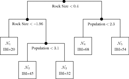
Figure 12.7 shows a typical tree. Four binary questions are represented by splits in the tree. Each split is based on the value of one of the predictors. The left branch of a split is taken when the answer is yes, so that the condition labeling that split is met. For example, the top split indicates that the left portion of the tree is for those observations with rock size values of 0.4 or less (sand and smaller). Each position in the tree where a split is made is a parent node. The topmost parent node is called the root node. All parent nodes except the root node are internal nodes. At the bottom of the tree the data have been classified into five terminal nodes based on the decisions made at the parent nodes. Associated with each terminal node is the mean value of the IBI for all observations in that node. We would use this value as the prediction for any observation whose predictors lead to this node. For example, we predict IBI = 20 for any observation that would be classified in .

Figure 12.7 Tree fit to predict IBI for Example 12.4. The root node is the top node of the tree, the parent nodes are the other nodes indicated by the • symbol, and the terminal nodes are . Follow the left branch from a parent node when the indicated criterion is true, and the right branch when it is false.

12.1.4.1 Recursive Partitioning Regression Trees

Suppose initially that the response variable is continuous. Then tree-based smoothing is often called recursive partitioning regression. Section 12.1.4.3 discusses prediction of categorical responses.

Consider predictor–response data where x_i is a vector of p predictors associated with a response Y_i, for i = 1, . . ., n. For simplicity, assume that all p predictors are continuous. Let q denote the number of terminal nodes in the tree to be fitted.

Tree-based predictions are piecewise constant. If the predictor values for the ith observation place it in the jth terminal node, then the ith predicted response equals a constant, . Thus, the tree-based smooth is

(12.18)

This model is fitted using a partitioning process that adaptively partitions predictor space into hyperrectangles, each corresponding to one terminal node. Once the partitioning is complete, is set equal to, say, the mean response value of cases falling in the jth terminal node.

Notice that this framework implies that there are a large number of possible trees whenever n and/or p are not trivially small. Any terminal node might be split to create a larger tree. The two branches from any parent node might be collapsed to convert the parent node to a terminal node, forming a subtree of the original tree. Any branch itself might be replaced by one based on a different predictor variable and/or criterion. The partitioning process used to fit a tree is described next.

In the simplest case, suppose q = 2. Then we seek to split into two hyperrectangles using one axis-parallel boundary. The choice can be characterized by a split coordinate, c {1, . . ., p}, and a split point or threshold, . The two terminal nodes are then and . Denote the sets of indices of the observations falling in the two nodes as and , respectively. Using node-specific sample averages yields the fit

(12.19)

where n_j is the number of observations falling in the jth terminal node.

For continuous predictors and ordered discrete predictors, defining a split in this manner is straightforward. Treatment of an unordered categorical variable is different. Suppose each observation of this variable may take on one of several categories. The set of all such categories must be partitioned into two subsets. Fortunately, we may avoid considering all possible partitions. First, order the categories in order of the average response within each category. Then, treat these ordered categories as if they were observations of an ordered discrete predictor. This strategy permits optimal splits [65]. There are also natural ways to deal with observations having some missing predictor values. Finally, selecting transformations of the predictors is usually not a problem: Tree-based models are invariant to monotone transformations of the predictors because the split point is determined in terms of the rank of predictor, in most software packages.

To find the best tree with q = 2 terminal nodes, we seek to minimize the residual squared error,

(12.20)

with respect to c and t, where . Note that the are defined using the values of c and t, and that RSS(c, t) changes only when memberships change in the sets . Minimizing (12.20) is therefore a combinatorial optimization problem. For each coordinate, we need to try at most n − 1 splits, and fewer if there are tied predictor values in the coordinate. Therefore, the minimal RSS(c, t) can be found by searching at most p(n − 1) trees. Exhaustive search to find the best tree is feasible when q = 2.

Now suppose q = 3. A first split coordinate and split point partition into two hyperrectangles. One of these hyperrectangles is then partitioned into two portions using a second split coordinate and split point, applied only within this hyperrectangle. The result is three terminal nodes. There are at most p(n − 1) choices for the first split. For making the second split on any coordinate different from the one used for the first split, there are at most p(n − 1) choices for each possible first split chosen. For a second split on the same coordinate as the first split, there are at most p(n − 2) choices. Carrying this logic on for larger q, we see that there are about (n − 1)(n − 2) . . . (n − q + 1)p^q−1 trees to be searched. This enormous number defies exhaustive search.

Instead, a greedy search algorithm is applied (see Section 3.2). Each split is treated sequentially. The best single split is chosen to split the root node. For each child node, a separate split is chosen to split it optimally. Note that the q terminal nodes obtained in this way will usually not minimize the residual squared error over the set of all possible trees having q terminal nodes.

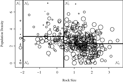
Example 12.5 (Stream Monitoring, Continued) To understand how terminal nodes in a tree correspond to hyperrectangles in predictor space, recall the stream monitoring data introduced in Example 12.4. Another representation of the tree in Figure 12.7 is given in Figure 12.8. This plot shows the partitioning of the predictor space determined by values of the rock size and population density variables. Each circle is centered at an x_i observation (i = 1, . . ., n). The area of each circle reflects the magnitude of the IBI value for that observation, with larger circles corresponding to larger IBI values. The rectangular regions labeled in this graph correspond to the terminal nodes shown in Figure 12.7. The first split (on the rock size coordinate at the threshold t = 0.4) is shown by the vertical line in the middle of the plot. Subsequent splits partition only portions of the predictor space. For example, the region corresponding to rock size exceeding 0.4 is next split into two nodes, and , based on the value of the population density variable. Note that sequential splitting has drawbacks: An apparently natural division of the data based on whether the population density exceeds about 2.5 is represented by two slightly mismatched splits because a previous split occurred at 0.4 on the rock size variable. The uncertainty of the tree structure is discussed further in Section 12.1.4.4.

Figure 12.8 Partitioning of predictor space (rock size and population density variables) for predicting IBI as discussed in Examples 12.4 and 12.5.

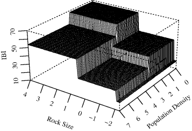
The piecewise constant model for this fitted tree is shown in Figure 12.9, with the IBI on the vertical axis. To best display the surface, the axes have been reversed compared to Figure 12.8.

Figure 12.9 Piecewise constant tree model predictions for IBI as discussed in Example 12.5.

12.1.4.2 Tree Pruning

For a given q, greedy search can be used to fit a tree model. Note that q is, in essence, a smoothing parameter. Large values of q retain high fidelity to the observed data but provide trees with high potential variation in predictions. Such an elaborate model may also sacrifice interpretability. Low values of q provide less predictive variability because there are only a few terminal nodes, but predictive bias may be introduced if responses are not homogeneous within each terminal node. We now discuss how to choose q.

A naive approach for choosing q is to continue splitting terminal nodes until no additional split gives a sufficient reduction in the overall residual sum of squares. This approach may miss important structure in the data because subsequent splits may be quite valuable even if the current split offers little or no improvement. For example, consider the saddle-shaped response surface obtained when X₁ and X₂ are independent predictors distributed uniformly over [− 1, 1] and Y = X₁X₂. Then no single split on either predictor variable will be of much benefit, but any first split enables two subsequent splits that will greatly reduce the residual sum of squares.

A more effective strategy for choosing q begins by growing the tree, splitting each terminal node until it has no more than some prespecified minimal number of observations in it or its residual squared error does not exceed some prespecified percentage of the squared error for the root node. The number of terminal nodes in this full tree may greatly exceed q. Then, terminal nodes are sequentially recombined from the bottom up a way that doesn't greatly inflate the residual sum of squares. One implementation of this strategy is called cost–complexity pruning [65, 540]. The final tree is a subtree of the full tree, selected according to a criterion that balances a penalty for prediction error and a penalty for tree complexity.

Let the full tree be denoted by T₀, and let T denote some subtree of T₀ that can be obtained by pruning everything below some parent nodes in T₀. Let q(T) denote the number of terminal nodes in the tree T. The cost–complexity criterion is given by

(12.21)

where r(T) is the residual sum of squares or some other measure of prediction error for tree T, and α is a user-supplied parameter that penalizes tree complexity. For a given α, the optimal tree is the subtree of T₀ that minimizes R_α(T). When α = 0, the full tree, T₀, will be selected as optimal. When α =∞, the tree with only the root node will be selected. If T₀ has q(T₀) terminal nodes, then there are at most q(T₀) subtrees that can be obtained by choosing different values of α.

The best approach for selecting the value for the parameter α in (12.21) relies on cross-validation. The dataset is partitioned into V separate portions of equal size, where V is typically between 3 and 10. For a finite sequence of α values, the algorithm proceeds as follows:

Repeat this process for all V parts of the data. For each α, compute the total cross-validated sum of squares over all V data partitions. The value of α that minimizes the cross-validated sum of squares is selected; call it . Having estimated the best value for the complexity parameter, we may now prune the full tree for all the data back to the subtree determined by .

Efficient algorithms for finding the optimal tree for a sequence of α values (see step 2 above) are available [65, 540]. Indeed, the set of optimal trees for a sequence of α values is nested, with smaller trees corresponding to larger values of α, and all members in the sequence can be visited by sequential recombination of terminal nodes from the bottom up. Various enhancements of this cross-validation strategy have been proposed, including a variant of the above approach that chooses the simplest tree among those trees that nearly achieve the minimum cross-validated sum of squares [629].

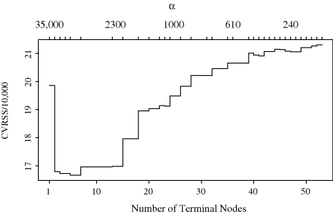
Example 12.6 (Stream Monitoring, Continued) Let us return to the stream ecology example introduced in Example 12.4. A full tree for these data was obtained by splitting until every terminal node has fewer than 10 observations in it or has residual squared error less 1% of the residual squared error for the root node. This process produced a full tree with 53 terminal nodes. Figure 12.10 shows the total cross-validated residual squared error as a function of the number of terminal nodes. This plot was produced using 10-fold cross-validation (V = 10). The full tree can be pruned from the bottom up, recombining the least beneficial terminal nodes, until the minimal value of R_α(T) is reached. Note that the correspondence between values of α and tree sizes means that we need only consider a limited collection of α values, and it is therefore more straightforward to plot R_α(T) against q(T) instead of plotting against α. The minimal cross-validated sum of squares is achieved for a tree with five terminal nodes; indeed, this is the tree shown in Figure 12.7.

Figure 12.10 Cross-validation residual sum of squares versus node size for Example 12.6. The top horizonal axis shows the cost–complexity parameter α.

For this example, the selection of the optimal α, and thus the final tree, varies with different random partitions of the data. The optimal tree typically has between 3 and 13 terminal nodes. This uncertainty emphasizes the potential structural instability of tree-based models, particularly for datasets where the signal is not strong.

12.1.4.3 Classification Trees

Digressing briefly from this chapter's focus on smoothing, it is worthwhile here to quickly summarize tree-based methods for categorical response variables.

Recursive partitioning models for predicting a categorical response variable are typically called classification trees [65, 540]. Let each response observation Y_i take on one of M categories. Let denote the proportion of observations in the terminal node that are of class m (for m = 1, . . ., M). Loosely speaking, all the observations in are predicted to equal the class that makes up the majority in that node. Such prediction by majority vote within terminal nodes can be modified in two ways. First, votes can be weighted to reflect prior information about the overall prevalence of each class. This permits predictions to be biased toward predominant classes. Second, votes can be weighted to reflect different losses for different types of misclassification [629]. For example, if classes correspond to medical diagnoses, some false positive or false negative diagnoses may be grave errors, while other mistakes may have only minor consequences.

Construction of a classification tree relies on partitioning the predictor space using a greedy strategy similar to the one used for recursive partitioning regression. For a regression tree split, the split coordinate c and split point t are selected by minimizing the total residual sum of squares within the left and right children nodes. For classification trees, a different measure of error is required. The residual squared error is replaced by a measure of node impurity.

There are various approaches to measuring node impurity, but most are based on the following principle. The impurity of node j should be small when observations in that node are concentrated within one class, and the impurity should be large when they are distributed uniformly over all M classes. Two popular measures of impurity are the entropy, given for node j by , and the Gini index, given by . These approaches are more effective than simply counting misclassifications because a split may drastically improve the purity in a node without changing any classifications. This occurs, for example, when majority votes on both sides of a split have the same outcome as the unsplit vote, but the margin of victory in one of the subregions is much narrower than in the other.

Cost–complexity tree pruning can proceed using the same strategies described in Section 12.1.4.2. The entropy or the Gini index can be used for the cost measure r(T) in (12.21). Alternatively, one may let r(T) equal a (possibly weighted) misclassification rate to guide pruning.

12.1.4.4 Other Issues for Tree-Based Methods

Tree-based methods offer several advantages over other, more traditional modeling approaches. First, tree models fit interactions between predictors and other nonadditive behavior without requiring formal specification of the form of the interaction by the user. Second, there are natural ways to use data with some missing predictor values, both when fitting the model and when using it to make predictions. Some strategies are surveyed in [64, 540].

One disadvantage is that trees can be unstable. Therefore, care must be taken not to overinterpret particular splits. For example, if the two smallest IBI values in in Figure 12.8 are increased somewhat, then this node is omitted when a new tree is constructed on the revised data. New data can often cause quite different splits to be chosen even if predictions remain relatively unchanged. For example, from Figure 12.8 it is easy to imagine that slightly different data could have led to the root node splitting on population density at the split point 2.5, rather than on rock size at the point 0.4. Trees can also be unstable in that building the full tree to a different size before pruning can cause a different optimal tree to be chosen after pruning.

Another concern is that assessment of uncertainty can be somewhat challenging. There is no simple way to summarize a confidence region for the tree structure itself. Confidence intervals for tree predictions can be obtained using the bootstrap (Chapter 9).

Tree-based methods are popular in computer science, particular for classification [522, 540]. Bayesian alternatives to tree methods have also been proposed [112, 151]. Medical applications of tree-based methods are particularly popular, perhaps because the binary decision tree is simple to explain and to apply as a tool in disease diagnosis [65, 114].

12.2 General Multivariate Data

Finally, we consider high-dimensional data that lie near a low-dimensional manifold such as a curve or surface. For such data, there may be no clear conceptual separation of the variables into predictors and responses. Nevertheless, we may be interested in estimating smooth relationships among variables. In this section we describe one approach, called principal curves, for smoothing multivariate data. Alternative methods for discovering relationships among variables, such as association rules and cluster analysis, are discussed in [323].

12.2.1 Principal Curves

A principal curve is a special type of one-dimensional nonparametric summary of a p-dimensional general multivariate dataset. Loosely speaking, each point on a principal curve is the average of all data that project onto that point on the curve. We began motivating principal curves in Section 11.6. The data in Figure 11.18 were not suitable for predictor–response smoothing, yet adapting the concept of smoothing to general multivariate data allowed the very good fit shown in the right panel of Figure 11.18. We now describe more precisely the notion of a principal curve and its estimation [321]. Related software includes [319, 367, 644].

12.2.1.1 Definition and Motivation

General multivariate data may lie near a connected, one-dimensional curve snaking through . It is this curve we want to estimate. We adopt a time–speed parameterization of curves below to accommodate the most general case.

We can write a one-dimensional curve in as f(τ) = (f₁(τ), . . ., f_p(τ)) for τ between τ₀ and τ₁. Here, τ can be used to indicate distance along the one-dimensional curve in p-dimensional space. The arc length of a curve f is , where

If ||f′(τ)|| = 1 for all τ [τ₀, τ₁], then the arc length between any two points τ_a and τ_b along the curve is |τ_a − τ_b|. In this case, f is said to have the unit-speed parameterization. It is often helpful to imagine a bug walking forward along the curve at a speed of 1 or backward with at a speed of −1 (the designation of forward and backward is arbitrary). Then the amount of time it takes the bug to walk between two points corresponds to the arc length, and the positive or negative sign corresponds to the direction taken. Any smooth curve with ||f′(τ)|| > 0 for all τ [τ₀, τ₁] can be reparameterized to unit speed. If the coordinate functions of a unit-speed curve are smooth, then f itself is smooth.

The types of curves we are interested in estimating are smooth, nonintersecting, curves that aren't too wiggly. Specifically, let us assume that f is a smooth unit-speed curve in parameterized over the closed interval [τ₀, τ₁] such that f(t) ≠ f(r) when r ≠ t for all r, t [τ₀, τ₁], and f has finite length inside any closed ball in .

For any point , define the projection index function as according to

(12.22)

Thus τ_f(x) is the largest value of τ for which f(τ) is closest to x. Points with similar projection indices project orthogonally onto a small portion of the curve f. The projection index will later be used to define neighborhoods.

Suppose that X is a random vector in , having a probability density with finite second moment. Unlike in previous sections, we cannot distinguish variables as predictors and response.

We define f to be a principal curve if for all τ^∗ [τ₀, τ₁]. This requirement is sometimes termed self-consistency. Figure 12.11 illustrates this notion that the distribution of points orthogonal to the curve at some τ must have mean equal to the curve itself at that point. In the left panel, a distribution is sketched along an axis that is orthogonal to f at one τ^∗. The mean of this density is f(τ^∗). Note that for ellipsoid distributions, the principal component lines are principal curves. Principal components are reviewed in [471].

Figure 12.11 Two panels illustrating the definition of a principal curve and its estimation. In the left panel, the curve f is intersected by an axis that is orthogonal to f at a particular τ^∗. A conditional density curve is sketched over this axis; if f is a principal curve, then the mean of this conditional density must equal f(τ^∗). In the right panel, a neighborhood around τ^∗ is sketched. Within these boundaries, all points project onto f near τ^∗. The sample mean of these points should be a good approximation to the true mean of the conditional density in the left panel.

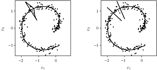
Principal curves are motivated by the concept of local averaging: The principal curve connects the means of points in local neighborhoods. For predictor–response smooths, neighborhoods are defined along the predictor coordinate axes. For principal curves, neighborhoods are defined along the curve itself. Points that project nearby on the curve are in the same neighborhood. The right panel of Figure 12.11 illustrates the notion of a local neighborhood along the curve.

12.2.1.2 Estimation

An iterative algorithm can be used to estimate a principal curve from a sample of p-dimensional data, X₁, . . ., X_n. The algorithm is initialized at iteration t = 0 by choosing a simple starting curve and setting from (12.22). One reasonable choice would be to set , where a is the first linear principal component estimated from the data. The algorithm proceeds as follows:

1. Smooth the kth coordinate of the data. Specifically, for k = 1, . . ., p, smooth X_ik against τ^(t)(X_i) using a standard bivariate predictor–response smoother with span h^(t). The projection of the points X_i onto for i = 1, . . ., n provides the predictors τ^(t)(X_i). The responses are the X_ik. The result is , which serves as an estimate of E{X|τ^(t)(x)}. This implements the scatterplot smoothing strategy of locally averaging the collection of points that nearly project onto the same point on the principal curve.

2. Interpolate between the for i = 1, . . ., n, and compute as the distances along . Note that some X_i may project onto a quite different segment than they did at the previous iteration.

3. Let τ^(t+1)(X) equal transformed to unit speed. This amounts to rescaling the so that each equals the total distance traveled along the polygonal curve to reach it.

4. Evaluate the convergence of , and stop if possible; otherwise, increment t and return to step 1. A relative convergence criterion could be constructed based on the total error, .

The result of this algorithm is a piecewise linear polygonal curve that serves as the estimate of the principal curve.

The concept of principal curves can be generalized for multivariate responses. For this purpose, principal surfaces are defined analogously to the above. The surface is parameterized by a vector τ, and data points are projected onto the surface. Points that project anywhere on the surface near τ^∗ dominate in the local smooth at τ^∗.

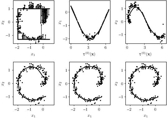
Example 12.7 (Principal Curve for Bivariate Data) Figure 12.12 illustrates several steps during the iterative process of fitting a principal curve. The sequence of panels should be read across the page from top left to bottom right. In the first panel, the data are plotted. The solid line shaped like a square letter C is . Each data point is connected to by a line showing its orthogonal projection. As a bug walks along from the top right to the bottom right, τ⁽⁰⁾(x) increases from 0 to about 7. The second and third panels show each coordinate of the data plotted against the projection index, τ⁽⁰⁾(x). These coordinatewise smooths correspond to step 1 of the estimation algorithm. A smoothing spline was used in each panel, and the resulting overall estimate, , is shown in the fourth panel. The fifth panel shows . The sixth panel gives the final result when convergence was achieved.

Figure 12.12 These panels illustrate the progression of the iterative fit of a principal curve. See Example 12.7 for details.

12.2.1.3 Span Selection

The principal curve algorithm depends on the selection of a span h^(t) at each iteration. Since the smoothing is done coordinatewise, different spans could be used for each coordinate at each iteration, but in practice it is more sensible to standardize the data before analysis and then use a common h^(t).

Nevertheless, the selection of h^(t) from one iteration to the next remains an issue. The obvious solution is to select h^(t) via cross-validation at each iteration. Surprisingly, this doesn't work well. Pervasive undersmoothing arises because the errors in the coordinate functions are autocorrelated. Instead, h^(t) = h can be chosen sensibly and remain unchanged until convergence is achieved. Then, one additional iteration of step 1 can be done with a span chosen by cross-validation.

This span selection approach is troubling because the initial span choice clearly can affect the shape of the curve to which the algorithm converges. When the span is then cross-validated after convergence, it is too late to correct for such an error. Nevertheless, the algorithm seems to work well on a variety of examples where ordinary smoothing techniques would fail catastrophically.

problems

12.1. For A defined as in (12.5), smoothing matrices S_k, and n-vectors γ_k for k = 1, . . ., p, let be the space spanned by vectors that pass through S_k unchanged (i.e., vectors v satisfying S_kv = v). Prove that Aγ = 0 (where γ = (γ₁ γ₂ . . . γ_p)^T) if and only if for all k and .

12.2. Accurate measurement of body fat can be expensive and time consuming. Good models to predict body fat accurately using standard measurements are still useful in many contexts. A study was conducted to predict body fat using 13 simple body measurements on 251 men. For each subject, the percentage of body fat as measured using an underwater weighing technique, age, weight, height, and 10 body circumference measurements were recorded (Table 12.2). Further details on this study are available in [331, 354]. These data are available from the website for this book. The goal of this problem is to compare and contrast several multivariate smoothing methods applied to these data.

Table 12.2 Potential predictors of body fat. Predictors 4–13 are circumference measurements given in centimeters.

a. Using a smoother of your own choosing, develop a backfitting algorithm to fit an additive model to these data as described in Section 12.1.1. Compare the results of the additive model with those from a multiple regression model.

b. Use any available software to estimate models for these data, using five methods: (1) the standard multiple linear regression (MLR) model, (2) an additive model (AM), (3) projection pursuit regression (PPR), (4) the alternating conditional expectations (ACE) procedure, and (5) the additivity and variance stabilization (AVAS) approach.

i. For MLR, AM, ACE, and AVAS, plot the kth estimated coordinate smooth against the observed values of the kth predictor for k = 1, . . ., 13. In other words, graph the values of versus x_ik for i = 1, . . ., 251 as in Figure 12.2. For PPR, imitate Figure 12.6 by plotting each component smooth against the projection coordinate. For all methods, include the observed data points in an appropriate way in each graph. Comment on any differences between the methods.

ii. Carry out leave-one-out cross-validation analyses where the ith cross-validated residual is computed as the difference between the ith observed response and the ith predicted response obtained when the model is fitted omitting the ith data point from the dataset. Use these results to compare the predictive performance of MLR, AM, and PPR using a cross-validated residual sum of squares similar to (11.16).

12.3. For the body fat data of Problem 12.2, compare the performance of at least three different smoothers used within an additive model of the form given in (12.3). Compare the leave-one-out cross-validation mean squared prediction error for the different smoothers. Is one smoother superior to another in the additive model?

12.4. Example 2.5 describes a generalized linear model for data derived from testing an algorithm for human face recognition. The data are available from the book website. The response variable is binary, with Y_i = 1 if two images of the same person were correctly matched and Y_i = 0 otherwise. There are three predictor variables. The first is the absolute difference in eye region mean pixel intensity between the two images of the ith person. The second is the absolute difference in nose–cheek region mean pixel intensity between the two images. The third predictor compares pixel intensity variability between the two images. For each image of the ith person, the median absolute deviation (a robust spread measure) of pixel intensity is computed in two image areas: the forehead and nose–cheek regions. The third predictor is the between-image ratio of these within-image ratios. Fit a generalized additive model to these data. Plot your results and interpret. Compare your results with the fit of an ordinary logistic regression model.

12.5. Consider a larger set of stream monitoring predictors of the index of biotic integrity for macroinvertebrates considered in Example 12.4. The 21 predictors, described in more detail in the website for this book, can be grouped into four categories:

12.6. Discuss how the combinatorial optimization methods from Chapter 3 might be used to improve tree-based methods.

12.7. Find an example for which X = f(τ) + , where is a random vector with mean zero, but f is not a principal curve for X.

12.8. The website for this book provides some artificial data suitable for fitting a principal curve. There are 50 observations of a bivariate variable, and each coordinate has been standardized. Denote these data as x₁, . . ., x₅₀.

a. Plot the data. Let correspond to the segment of the line through the origin with slope 1 onto which the data project. Superimpose this line on the graph. Imitating the top left panel of Figure 12.12, show how the data project onto .

b. Compute τ⁽⁰⁾(x_i) for each data point x_i. Transform to unit speed. Hint: Show why the transformation a^Tx_i works, where .

c. For each coordinate of the data in turn, plot the data values for that coordinate (i.e., the x_ik values for i = 1, . . ., 50 and k = 1 or k = 2) against the projection index values, τ⁽⁰⁾(x_i). Smooth the points in each plot, and superimpose the smooth on each graph. This mimics the center and right top panels of Figure 12.12.

d. Superimpose over a scatterplot of the data, as in the bottom left panel of Figure 12.12.

e. Advanced readers may consider automating and extending these steps to produce an iterative algorithm whose iterates converges to the estimated principal curve. Some related software for fitting principal curves is available as packages for R (www.r-project.org).