
Chapter 5
Numerical Integration
Consider a one-dimensional integral of the form ![]() . The value of the integral can be derived analytically for only a few functions f. For the rest, numerical approximations of the integral are often useful. Approximation methods are well known by both numerical analysts [139, 353, 376, 516] and statisticians [409, 630].
. The value of the integral can be derived analytically for only a few functions f. For the rest, numerical approximations of the integral are often useful. Approximation methods are well known by both numerical analysts [139, 353, 376, 516] and statisticians [409, 630].
Approximation of integrals is frequently required for Bayesian inference since a posterior distribution may not belong to a familiar distributional family. Integral approximation is also useful in some maximum likelihood inference problems when the likelihood itself is a function of one or more integrals. An example of this occurs when fitting generalized linear mixed models, as discussed in Example 5.1.
To initiate an approximation of ![]() , partition the interval [a, b] into n subintervals, [xi, xi+1] for i = 0, . . ., n − 1, with x0 = a and xn = b. Then
, partition the interval [a, b] into n subintervals, [xi, xi+1] for i = 0, . . ., n − 1, with x0 = a and xn = b. Then ![]() . This composite rule breaks the whole integral into many smaller parts, but postpones the question of how to approximate any single part.
. This composite rule breaks the whole integral into many smaller parts, but postpones the question of how to approximate any single part.
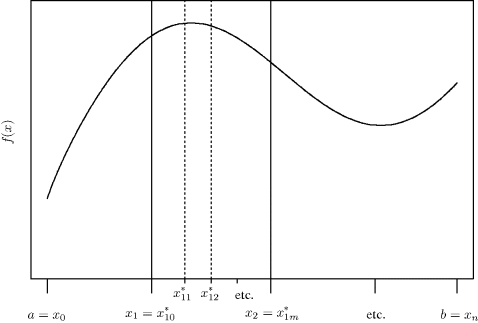
The approximation of a single part will be made using a simple rule. Within the interval [xi, xi+1], insert m + 1 nodes, ![]() for j = 0, . . ., m. Figure 5.1 illustrates the relationships among the interval [a, b], the subintervals, and the nodes. In general, numerical integration methods require neither equal spacing of subintervals or nodes nor equal numbers of nodes within each subinterval.
for j = 0, . . ., m. Figure 5.1 illustrates the relationships among the interval [a, b], the subintervals, and the nodes. In general, numerical integration methods require neither equal spacing of subintervals or nodes nor equal numbers of nodes within each subinterval.
Figure 5.1 To integrate f between a and b, the interval is partitioned into n subintervals, [xi, xi+1], each of which is further partitioned using m + 1 nodes, ![]() . Note that when m = 0, the subinterval [xi, xi+1] contains only one interior node,
. Note that when m = 0, the subinterval [xi, xi+1] contains only one interior node, ![]() .
.
A simple rule will rely upon the approximation
for some set of constants Aij. The overall integral is then approximated by the composite rule that sums (5.1) over all subintervals.
5.1 Newton–Côtes Quadrature
A simple and flexible class of integration methods consists of the Newton–Côtes rules. In this case, the nodes are equally spaced in [xi, xi+1], and the same number of nodes is used in each subinterval. The Newton–Côtes approach replaces the true integrand with a polynomial approximation on each subinterval. The constants Aij are selected so that ![]() equals the integral of an interpolating polynomial on [xi, xi+1] that matches the value of f at the nodes within this subinterval. The remainder of this section reviews common Newton–Côtes rules.
equals the integral of an interpolating polynomial on [xi, xi+1] that matches the value of f at the nodes within this subinterval. The remainder of this section reviews common Newton–Côtes rules.
5.1.1 Riemann Rule
Consider the case when m = 0. Suppose we define ![]() , and
, and ![]() . The simple Riemann rule amounts to approximating f on each subinterval by a constant function,
. The simple Riemann rule amounts to approximating f on each subinterval by a constant function, ![]() , whose value matches that of f at one point on the interval. In other words,
, whose value matches that of f at one point on the interval. In other words,
The composite rule sums n such terms to provide an approximation to the integral over [a, b].
Suppose the xi are equally spaced so that each subinterval has the same length h = (b − a)/n. Then we may write xi = a + ih, and the composite rule is
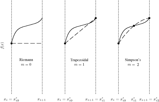
As Figure 5.2 shows, this corresponds to the Riemann integral studied in elementary calculus. Furthermore, there is nothing special about the left endpoints of the subintervals: We easily could have replaced ![]() with
with ![]() in (5.2) .
in (5.2) .
Figure 5.2 Approximation (dashed) to f (solid) provided on the subinterval [xi, xi+1], for the Riemann, trapezoidal, and Simpson's rules.
The approximation given by (5.3) converges to the true value of the integral as n→ ∞, by definition of the Riemann integral of an integrable function. If f is a polynomial of zero degree (i.e., a constant function), then f is constant on each subinterval, so the Riemann rule is exact.
When applying the composite Riemann rule, it makes sense to calculate a sequence of approximations, say ![]() , for an increasing sequence of numbers of subintervals, nk, as k = 1, 2, . . . . Then, convergence of
, for an increasing sequence of numbers of subintervals, nk, as k = 1, 2, . . . . Then, convergence of ![]() can be monitored using an absolute or relative convergence criterion as discussed in Chapter 2. It is particularly efficient to use nk+1 = 2nk so that half the subinterval endpoints at the next step correspond to the old endpoints from the previous step. This avoids calculations of f that are effectively redundant.
can be monitored using an absolute or relative convergence criterion as discussed in Chapter 2. It is particularly efficient to use nk+1 = 2nk so that half the subinterval endpoints at the next step correspond to the old endpoints from the previous step. This avoids calculations of f that are effectively redundant.
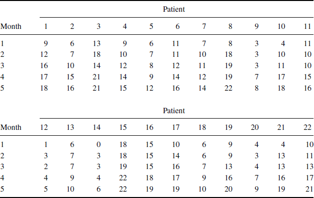
Example 5.1 (Alzheimer's Disease) Data from 22 patients with Alzheimer's disease, an ailment characterized by progressive mental deterioration, are shown in Table 5.1. In each of five consecutive months, patients were asked to recall words from a standard list given previously. The number of words recalled by each patient was recorded. The patients in Table 5.1 were receiving an experimental treatment with lecithin, a dietary supplement. It is of interest to investigate whether memory improved over time. The data for these patients (and 25 control cases) are available from the website for this book and are discussed further in [155].
Table 5.1 Words recalled on five consecutive monthly tests for 22 Alzheimer's patients receiving lecithin.
Consider fitting these data with a very simple generalized linear mixed model [69, 670]. Let Yij denote the number of words recalled by the ith individual in the jth month, for i = 1, . . ., 22 and j = 1, . . ., 5. Suppose Yij|λij have independent Poisson(λij) distributions, where the mean and variance of Yij is λij. Let xij = (1 j)T be a covariate vector: Aside from an intercept term, only the month is used as a predictor. Let β = (β0 β1)T be a parameter vector corresponding to x. Then we model the mean of Yij as
(5.4) ![]()
where the γi are independent ![]() random effects. This model allows separate shifts in λij on the log scale for each patient, reflecting the assumption that there may be substantial between-patient variation in counts. This is reasonable, for example, if the baseline conditions of patients prior to the start of treatment varied.
random effects. This model allows separate shifts in λij on the log scale for each patient, reflecting the assumption that there may be substantial between-patient variation in counts. This is reasonable, for example, if the baseline conditions of patients prior to the start of treatment varied.
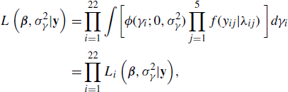
With this model, the likelihood is
where f(yij|λij) is the Poisson density, ![]() is the normal density function with mean zero and variance
is the normal density function with mean zero and variance ![]() , and Y is a vector of all the observed response values. The log likelihood is therefore
, and Y is a vector of all the observed response values. The log likelihood is therefore
where li denotes the contribution to the log likelihood made by data from the ith patient.
To maximize the log likelihood, we must differentiate l with respect to each parameter and solve the corresponding score equations. This will require a numerical root-finding procedure, since the solution cannot be determined analytically. In this example, we look only at one small portion of this overall process: the evaluation of dli/dβk for particular given values of the parameters and for a single i and k. This evaluation would be repeated for the parameter values tried at each iteration of a root-finding procedure.
Let i = 1 and k = 1. The partial derivative with respect to the parameter for monthly rate of change is dl1/dβ1 = (dL1/dβ1);/L1, where L1 is implicitly defined in (5.5). Further,
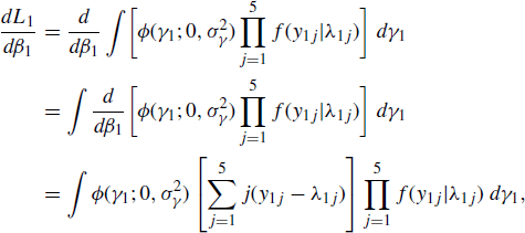
where λ1j = exp {β0 + jβ1 + γ1}. The last equality in (5.7) follows from standard analysis of generalized linear models [446].
Suppose, at the very first step of optimization, we start with initial values β = (1.804, 0.165) and ![]() . These starting values were chosen using simple exploratory analyses. Using these values for β and
. These starting values were chosen using simple exploratory analyses. Using these values for β and ![]() , the integral we seek in (5.7) has the integrand shown in Figure 5.3. The desired range of integration is the entire real line, whereas we have thus far only discussed integration over a closed interval. Transformations can be used to obtain an equivalent interval over a finite range (see Section 5.4.1), but to keep things simple here we will integrate over the range [− 0.07, 0.085], within which nearly all of the nonnegligible values of the integrand lie.
, the integral we seek in (5.7) has the integrand shown in Figure 5.3. The desired range of integration is the entire real line, whereas we have thus far only discussed integration over a closed interval. Transformations can be used to obtain an equivalent interval over a finite range (see Section 5.4.1), but to keep things simple here we will integrate over the range [− 0.07, 0.085], within which nearly all of the nonnegligible values of the integrand lie.
Figure 5.3 Example 5.1 seeks to integrate this function, which arises from a generalized linear mixed model for data on patients treated for Alzheimer's disease.
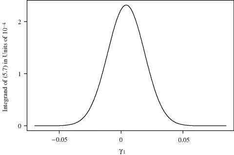
Table 5.2 shows the results of a series of Riemann approximations, along with running relative errors. The relative errors measure the change in the new estimated value of the integral as a proportion of the previous estimate. An iterative approximation strategy could be stopped when the magnitude of these errors falls below some predetermined tolerance threshold. Since the integral is quite small, a relative convergence criterion is more intuitive than an absolute criterion.
Table 5.2 Estimates of the integral in (5.7) using the Riemann rule with various numbers of subintervals. All estimates are multiplied by a factor of 105. Errors for use in a relative convergence criterion are given in the final column.
| Subintervals | Estimate | Relative Error |
| 2 | 3.49388458186769 | |
| 4 | 1.88761005959780 | −0.46 |
| 8 | 1.72890354401971 | −0.084 |
| 16 | 1.72889046749119 | −0.0000076 |
| 32 | 1.72889038608621 | −0.000000047 |
| 64 | 1.72889026784032 | −0.000000068 |
| 128 | 1.72889018400995 | −0.000000048 |
| 256 | 1.72889013551548 | −0.000000028 |
| 512 | 1.72889010959701 | −0.000000015 |
| 1024 | 1.72889009621830 | −0.0000000077 |
5.1.2 Trapezoidal Rule
Although the simple Riemann rule is exact if f is constant on [a, b], it can be quite slow to converge to adequate precision in general. An obvious improvement would be to replace the piecewise constant approximation by a piecewise mth-degree polynomial approximation. We begin by introducing a class of polynomials that can be used for such approximations. This permits the Riemann rule to be cast as the simplest member of a family of integration rules having increased precision as m increases. This family also includes the trapezoidal rule and Simpson's rule (Section 5.1.3).
Let the fundamental polynomials be
for j = 0, . . ., m. Then the function ![]() is an mth-degree polynomial that interpolates f at all the nodes
is an mth-degree polynomial that interpolates f at all the nodes ![]() in [xi, xi+1]. Figure 5.2 shows such interpolating polynomials for m = 0, 1, and 2.
in [xi, xi+1]. Figure 5.2 shows such interpolating polynomials for m = 0, 1, and 2.
These polynomials are the basis for the simple approximation
(5.9) ![]()
(5.10) ![]()
for ![]() . This approximation replaces integration of an arbitrary function f with polynomial integration. The resulting composite rule is
. This approximation replaces integration of an arbitrary function f with polynomial integration. The resulting composite rule is ![]() when there are m nodes on each subinterval.
when there are m nodes on each subinterval.
Letting m = 1 with ![]() and
and ![]() yields the trapezoidal rule. In this case,
yields the trapezoidal rule. In this case,
![]()
Integrating these polynomials yields ![]() . Therefore, the trapezoidal rule amounts to
. Therefore, the trapezoidal rule amounts to
(5.12) ![]()
When [a, b] is partitioned into n subintervals of equal length h = (b − a)/n, then the trapezoidal rule estimate is
The name of this approximation arises because the area under f in each subinterval is approximated by the area of a trapezoid, as shown in Figure 5.2. Note that f is approximated in any subinterval by a first-degree polynomial (i.e., a line) whose value equals that of f at two points. Therefore, when f itself is a line on [a, b], ![]() is exact.
is exact.
Example 5.2 (Alzheimer's Disease, Continued) For small numbers of subintervals, applying the trapezoidal rule to the integral from Example 5.1 yields similar results to those from the Riemann rule because the integrand is nearly zero at the endpoints of the integration range. For large numbers of subintervals, the approximation is somewhat better. The results are shown in Table 5.3.
Table 5.3 Estimates of the integral in (5.7) using the Trapezoidal rule with various numbers of subintervals. All estimates are multiplied by a factor of 105. Errors for use in a relative convergence criterion are given in the final column.
| Subintervals | Estimate | Relative Error |
| 2 | 3.49387751694744 | |
| 4 | 1.88760652713768 | −0.46 |
| 8 | 1.72890177778965 | −0.084 |
| 16 | 1.72888958437616 | −0.0000071 |
| 32 | 1.72888994452869 | 0.00000021 |
| 64 | 1.72889004706156 | 0.000000059 |
| 128 | 1.72889007362057 | 0.000000015 |
| 256 | 1.72889008032079 | 0.0000000039 |
| 512 | 1.72889008199967 | 0.00000000097 |
| 1024 | 1.72889008241962 | 0.00000000024 |
Suppose f has two continuous derivatives. Problem 5.1 asks you to show that
Subtracting the Taylor expansion of f about xi from (5.14) yields
and integrating (5.15) over [xi, xi+1] shows the approximation error of the trapezoidal rule on the ith subinterval to be ![]() . Thus
. Thus
(5.16) ![]()
(5.17) ![]()
(5.18) ![]()
for some ξ ![]() [a, b] by the mean value theorem for integrals. Hence the leading term of the overall error is
[a, b] by the mean value theorem for integrals. Hence the leading term of the overall error is ![]() .
.
5.1.3 Simpson's Rule
Letting m = 2, ![]() ,
, ![]() , and
, and ![]() in (5.8), we obtain Simpson's rule. Problem 5.2 asks you to show that
in (5.8), we obtain Simpson's rule. Problem 5.2 asks you to show that ![]() and
and ![]() . This yields the approximation
. This yields the approximation
(5.19) ![]()
for the (i + 1)th subinterval. Figure 5.2 shows how Simpson's rule provides a quadratic approximation to f on each subinterval.
Suppose the interval [a, b] has been partitioned into n subintervals of equal length h = (b − a)/n, where n is even. To apply Simpson's rule, we need an interior node in each [xi, xi+1]. Since n is even, we may adjoin pairs of adjacent subintervals, with the shared endpoint serving as the interior node of the larger interval. This provides n/2 subintervals of length 2h, for which
Example 5.3 (Alzheimer's Disease, Continued) Table 5.4 shows the results of applying Simpson's rule to the integral from Example 5.1. One endpoint and an interior node were evaluated on each subinterval. Thus, for a fixed number of subintervals, Simpson's rule requires twice as many evaluations of f as the Riemann or the trapezoidal rule. Following this example, we show that the precision of Simpson's rule more than compensates for the increased evaluations. From another perspective, if the number of evaluations of f is fixed at n for each method, we would expect Simpson's rule to outperform the previous approaches, if n is large enough.
Table 5.4 Estimates of the integral in (5.7) using Simpson's rule with various numbers of subintervals (and two nodes per subinterval). All estimates are multiplied by a factor of 105. Errors for use in a relative convergence criterion are given in the final column.
| Subintervals | Estimate | Relative Error |
| 2 | 1.35218286386776 | |
| 4 | 1.67600019467364 | 0.24 |
| 8 | 1.72888551990500 | 0.032 |
| 16 | 1.72889006457954 | 0.0000026 |
| 32 | 1.72889008123918 | 0.0000000096 |
| 64 | 1.72889008247358 | 0.00000000071 |
| 128 | 1.72889008255419 | 0.000000000047 |
| 256 | 1.72889008255929 | 0.0000000000029 |
| 512 | 1.72889008255961 | 0.00000000000018 |
| 1024 | 1.72889008255963 | 0.000000000000014 |
If f is quadratic on [a, b], then it is quadratic on each subinterval. Simpson's rule approximates f on each subinterval by a second-degree polynomial that matches f at three points; therefore the polynomial is exactly f. Thus, Simpson's rule exactly integrates quadratic f.
Suppose f is smooth—but not polynomial—and we have n subintervals [xi, xi+1] of equal length 2h. To assess the degree of approximation in Simpson's rule, we begin with consideration on a single subinterval, and denote the simple Simpson's rule on that subinterval as ![]() . Denote the true value of the integral on that subinterval as Ii.
. Denote the true value of the integral on that subinterval as Ii.
We use the Taylor series expansion of f about xi, evaluated at x = xi + h and x = xi + 2h, to replace terms in ![]() . Combining terms, this yields
. Combining terms, this yields
Now let ![]() . This function has the useful properties that
. This function has the useful properties that ![]() ,
, ![]() , and F′(x) = f(x). Taylor series expansion of F about xi, evaluated at x = xi + 2h, yields
, and F′(x) = f(x). Taylor series expansion of F about xi, evaluated at x = xi + 2h, yields
Subtracting (5.22) from (5.21) yields ![]() . This is the error for Simpson's rule on a single subinterval. Over the n subintervals that partition [a, b], the error is therefore the sum of such errors, namely
. This is the error for Simpson's rule on a single subinterval. Over the n subintervals that partition [a, b], the error is therefore the sum of such errors, namely ![]() . Note that Simpson's rule therefore exactly integrates cubic functions, too.
. Note that Simpson's rule therefore exactly integrates cubic functions, too.
5.1.4 General Kth-Degree Rule
The preceding discussion raises the general question about how to determine a Newton–Côtes rule that is exact for polynomials of degree k. This would require constants c0, . . ., ck that satisfy
(5.23) 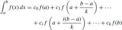
for any polynomial f. Of course, one could follow the derivations shown above for m = k, but there is another simple approach. If a method is to be exact for all polynomials of degree k, then it must be exact for particular—and easily integrated—choices like 1, x, x2, . . ., xk. Thus, we may set up a system of k equations in k unknowns as follows:
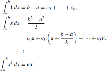
All that remains is to solve for the ci to derive the algorithm. This approach is sometimes called the method of undetermined coefficients.
5.2 Romberg Integration
In general, low-degree Newton–Côtes methods are slow to converge. However, there is a very efficient mechanism to improve upon a sequence of trapezoidal rule estimates. Let ![]() denote the trapezoidal rule estimate of
denote the trapezoidal rule estimate of ![]() using n subintervals of equal length h = (b − a)/n, as given in (5.13). Without loss of generality, suppose a = 0 and b = 1. Then
using n subintervals of equal length h = (b − a)/n, as given in (5.13). Without loss of generality, suppose a = 0 and b = 1. Then
(5.24) 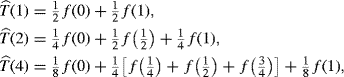
and so forth. Noting that
(5.25) ![]()
and so forth suggests the general recursion relationship
(5.27) ![]()
The Euler–Maclaurin formula (1.8) can be used to show that
for some constant c1, and hence
Therefore,
so the h2 error terms in (5.27) and (5.28) cancel. With this simple adjustment we have made a striking improvement in the estimate. In fact, the estimate given in (5.29) turns out to be Simpson's rule with subintervals of width h/2. Moreover, this strategy can be iterated for even greater gains.
Begin by defining ![]() for i = 0, . . ., m. Then define a triangular array of estimates like
for i = 0, . . ., m. Then define a triangular array of estimates like
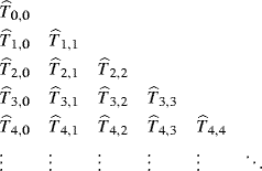
using the relationship
for j = 1, . . ., i and i = 1, . . ., m. Note that (5.30) can be reexpressed to calculate ![]() by adding an increment equal to 1/(4j − 1) times the difference
by adding an increment equal to 1/(4j − 1) times the difference ![]() to the estimate given by
to the estimate given by ![]() .
.
If f has 2m continuous derivatives on [a, b], then the entries in the mth row of the array have error ![]() for j ≤ m [121, 376]. This is such fast convergence that very small m will often suffice.
for j ≤ m [121, 376]. This is such fast convergence that very small m will often suffice.
It is important to check that the Romberg calculations do not deteriorate as m is increased. To do this, consider the quotient
(5.31) ![]()
The error in ![]() is attributable partially to the approximation strategy itself and partially to numerical imprecision introduced by computer roundoff. As long as the former source dominates, the Qij values should approach 4j+1 as i increases. However, when computer roundoff error is substantial relative to approximation error, the Qij values will become erratic. The columns of the triangular array of
is attributable partially to the approximation strategy itself and partially to numerical imprecision introduced by computer roundoff. As long as the former source dominates, the Qij values should approach 4j+1 as i increases. However, when computer roundoff error is substantial relative to approximation error, the Qij values will become erratic. The columns of the triangular array of ![]() can be examined to determine the largest j for which the quotients appear to approach 4j+1 before deteriorating. No further column should be used to calculate an update via (5.30). The following example illustrates the approach.
can be examined to determine the largest j for which the quotients appear to approach 4j+1 before deteriorating. No further column should be used to calculate an update via (5.30). The following example illustrates the approach.
Example 5.4 (Alzheimer's Disease, Continued) Table 5.5 shows the results of applying Romberg integration to the integral from Example 5.1. The right columns of this table are used to diagnose the stability of the Romberg calculations. The top portion of the table corresponds to j = 0, and the ![]() are the trapezoidal rule estimates given in Table 5.3. After some initial steps, the quotients in the top portion of the table converge nicely to 4. Therefore, it is safe and advisable to apply (5.30) to generate a second column of the triangular array. It is safe because the convergence of the quotients to 4 implies that computer roundoff error has not yet become a dominant source of error. It is advisable because incrementing one of the current integral estimates by one-third of the corresponding difference would yield a noticeably different updated estimate.
are the trapezoidal rule estimates given in Table 5.3. After some initial steps, the quotients in the top portion of the table converge nicely to 4. Therefore, it is safe and advisable to apply (5.30) to generate a second column of the triangular array. It is safe because the convergence of the quotients to 4 implies that computer roundoff error has not yet become a dominant source of error. It is advisable because incrementing one of the current integral estimates by one-third of the corresponding difference would yield a noticeably different updated estimate.
Table 5.5 Estimates of the integral in (5.7) using Romberg integration. All estimates and differences are multiplied by a factor of 105. The final two columns provide performance evaluation measures discussed in the text.
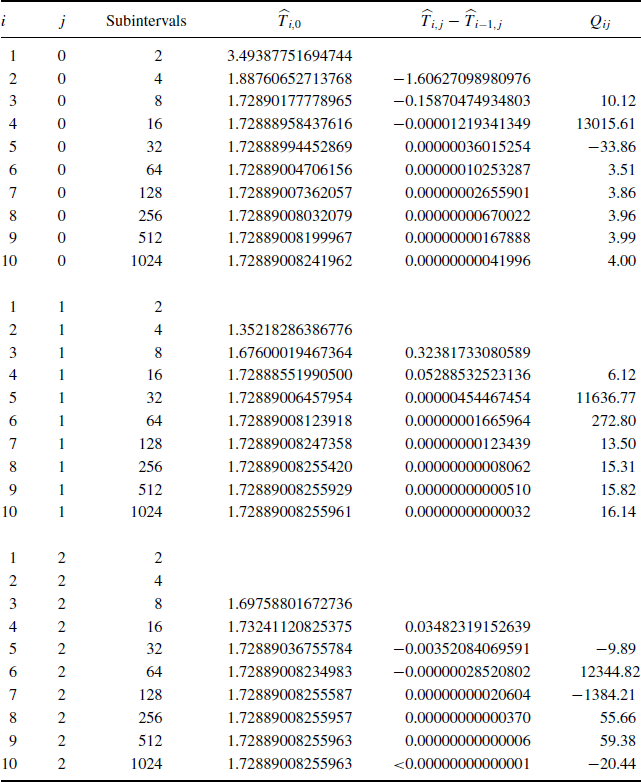
The second column of the triangular array is shown in the middle portion of Table 5.5. The quotients in this portion also appear reasonable, so the third column is calculated and shown in the bottom portion of the table. The values of Qi2 approach 64, allowing more tolerance for larger j. At i = 10, computer roundoff error appears to dominate approximation error because the quotient departs from near 64. However, note that incrementing the integral estimate by ![]() of the difference at this point would have a negligible impact on the updated estimate itself. Had we proceeded one more step with the reasoning that the growing amount of roundoff error will cause little harm at this point, we would have found that the estimate was not improved and the resulting quotients clearly indicated that no further extrapolations should be considered.
of the difference at this point would have a negligible impact on the updated estimate itself. Had we proceeded one more step with the reasoning that the growing amount of roundoff error will cause little harm at this point, we would have found that the estimate was not improved and the resulting quotients clearly indicated that no further extrapolations should be considered.
Thus, we may take ![]() to be the estimated value of the integral. In this example, we calculated the triangular array one column at a time, for m = 10. However, in implementation it makes more sense to generate the array one row at a time. In this case, we would have stopped after i = 9, obtaining a precise estimate with fewer subintervals—and fewer evaluations of f—than in any of the previous examples.
to be the estimated value of the integral. In this example, we calculated the triangular array one column at a time, for m = 10. However, in implementation it makes more sense to generate the array one row at a time. In this case, we would have stopped after i = 9, obtaining a precise estimate with fewer subintervals—and fewer evaluations of f—than in any of the previous examples.
The Romberg strategy can be applied to other Newton–Côtes integration rules. For example, if ![]() is the Simpson's rule estimate of
is the Simpson's rule estimate of ![]() using n subintervals of equal length, then the analogous result to (5.29) is
using n subintervals of equal length, then the analogous result to (5.29) is
(5.32) ![]()
Romberg integration is a form of a more general strategy called Richardson extrapolation [325, 516].
5.3 Gaussian Quadrature
All the Newton–Côtes rules discussed above are based on subintervals of equal length. The estimated integral is a sum of weighted evaluations of the integrand on a regular grid of points. For a fixed number of subintervals and nodes, only the weights may be flexibly chosen; we have limited attention to choices of weights that yield exact integration of polynomials. Using m + 1 nodes per subinterval allowed mth-degree polynomials to be integrated exactly.
An important question is the amount of improvement that can be achieved if the constraint of evenly spaced nodes and subintervals is removed. By allowing both the weights and the nodes to be freely chosen, we have twice as many parameters to use in the approximation of f. If we consider that the value of an integral is predominantly determined by regions where the magnitude of the integrand is large, then it makes sense to put more nodes in such regions. With a suitably flexible choice of m + 1 nodes, x0, . . ., xm, and corresponding weights, A0, . . ., Am, exact integration of 2(m + 1)th-degree polynomials can be obtained using ![]() .
.
This approach, called Gaussian quadrature, can be extremely effective for integrals like ![]() where
where ![]() is a nonnegative function and
is a nonnegative function and ![]() for all k ≥ 0. These requirements are reminiscent of density function with finite moments. Indeed, it is often useful to think of
for all k ≥ 0. These requirements are reminiscent of density function with finite moments. Indeed, it is often useful to think of ![]() as a density, in which case integrals like expected values and Bayesian posterior normalizing constants are natural candidates for Gaussian quadrature. The method is more generally applicable, however, by defining
as a density, in which case integrals like expected values and Bayesian posterior normalizing constants are natural candidates for Gaussian quadrature. The method is more generally applicable, however, by defining ![]() and applying the method to
and applying the method to ![]() .
.
The best node locations turn out to be the roots of a set of orthogonal polynomials that is determined by ![]() .
.
5.3.1 Orthogonal Polynomials
Some background on orthogonal polynomials is needed to develop Gaussian quadrature methods [2, 139, 395, 620]. Let pk(x) denote a generic polynomial of degree k. For convenience in what follows, assume that the leading coefficient of pk(x) is positive.
If ![]() , then the function f is said to be square-integrable with respect to
, then the function f is said to be square-integrable with respect to ![]() on [a, b]. In this case we will write
on [a, b]. In this case we will write ![]() . For any f and g in
. For any f and g in ![]() , their inner product with respect to
, their inner product with respect to ![]() on [a, b] is defined to be
on [a, b] is defined to be
(5.33) ![]()
If ![]() , then f and g are said to be orthogonal with respect to
, then f and g are said to be orthogonal with respect to ![]() on [a, b]. If also f and g are scaled so that
on [a, b]. If also f and g are scaled so that ![]() , then f and g are orthonormal with respect to
, then f and g are orthonormal with respect to ![]() on [a, b].
on [a, b].
Given any ![]() that is nonnegative on [a, b], there exists a sequence of polynomials
that is nonnegative on [a, b], there exists a sequence of polynomials ![]() that are orthogonal with respect to
that are orthogonal with respect to ![]() on [a, b]. This sequence is not unique without some form of standardization because
on [a, b]. This sequence is not unique without some form of standardization because ![]() implies
implies ![]() for any constant c. The canonical standardization for a set of orthogonal polynomials depends on
for any constant c. The canonical standardization for a set of orthogonal polynomials depends on ![]() and will be discussed later; a common choice is to set the leading coefficient of pk(x) equal to 1. For use in Gaussian quadrature, the range of integration is also customarily transformed from [a, b] to a range [a*, b*] whose choice depends on
and will be discussed later; a common choice is to set the leading coefficient of pk(x) equal to 1. For use in Gaussian quadrature, the range of integration is also customarily transformed from [a, b] to a range [a*, b*] whose choice depends on ![]() .
.
A set of standardized, orthogonal polynomials can be summarized by a recurrence relation
for appropriate choices of αk, βk, and γk that vary with k and ![]() .
.
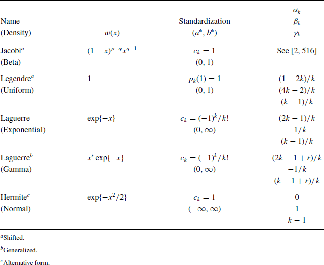
The roots of any polynomial in such a standardized set are all in (a*, b*). These roots will serve as nodes for Gaussian quadrature. Table 5.6 lists several sets of orthogonal polynomials, their standardizations, and their correspondences to common density functions.
Table 5.6 Orthogonal polynomials, their standardizations, their correspondence to common density functions, and the terms used for their recursive generation. The leading coefficient of a polynomial is denoted ck. In some cases, variants of standard definitions are chosen for best correspondence with familiar densities.
5.3.2 The Gaussian Quadrature Rule
Standardized orthogonal polynomials like (5.34) are important because they determine both the weights and the nodes for a Gaussian quadrature rule based on a chosen ![]() . Let
. Let ![]() be a sequence of orthonormal polynomials with respect to
be a sequence of orthonormal polynomials with respect to ![]() on [a, b] for a function
on [a, b] for a function ![]() that meets the conditions previously discussed. Denote the roots of pm+1(x) by a < x0 . . . xm < b. Then there exist weights A0, . . ., Am such that:
that meets the conditions previously discussed. Denote the roots of pm+1(x) by a < x0 . . . xm < b. Then there exist weights A0, . . ., Am such that:
(5.35) ![]()
The proof of this result may be found in [139].
Although this result and Table 5.6 provide the means by which the nodes and weights for an (m + 1)-point Gaussian quadrature rule can be calculated, one should be hesitant to derive these directly, due to potential numerical imprecision. Numerically stable calculations of these quantities can be obtained from publicly available software [228, 489]. Alternatively, one can draw the nodes and weights from published tables like those in [2, 387]. Lists of other published tables are given in [139, 630].
Of the choices in Table 5.6, Gauss–Hermite quadrature is particularly useful because it enables integration over the entire real line. The prominence of normal distributions in statistical practice and limiting theory means that many integrals resemble the product of a smooth function and a normal density; the usefulness of Gauss–Hermite quadrature in Bayesian applications is demonstrated in [478].
Example 5.5 (Alzheimer's Disease, Continued) Table 5.7 shows the results of applying Gauss–Hermite quadrature to estimate the integral from Example 5.1. Using the Hermite polynomials in this case is particularly appealing because the integrand from Example 5.1 really should be integrated over the entire real line, rather than the interval (− 0.07, 0.085). Convergence was extremely fast: With 8 nodes we obtained a relative error half the magnitude of that achieved by Simpson's rule with 1024 nodes. The estimate in Table 5.7 differs from previous examples because the range of integration differs. Applying Gauss–Legendre quadrature to estimate the integral over the interval (− 0.07, 0.085) yields an estimate of 1.72889008255962×10⁻⁵ using 26 nodes.
Table 5.7 Estimates of the integral in (5.7) using Gauss–Hermite quadrature with various numbers of nodes. All estimates are multiplied by a factor of 105. Errors for use in a relative convergence criterion are given in the final column.
| Nodes | Estimate | Relative Error |
| 2 | 1.72893306163335 | |
| 3 | 1.72889399083898 | −0.000023 |
| 4 | 1.72889068827101 | −0.0000019 |
| 5 | 1.72889070910131 | 0.000000012 |
| 6 | 1.72889070914313 | 0.000000000024 |
| 7 | 1.72889070914166 | −0.00000000000085 |
| 8 | 1.72889070914167 | −0.0000000000000071 |
Gaussian quadrature is quite different from the Newton–Côtes rules discussed previously. Whereas the latter rely on potentially enormous numbers of nodes to achieve sufficient precision, Gaussian quadrature is often very precise with a remarkably small number of nodes. However, for Gaussian quadrature the nodes for an m-point rule are not usually shared by an (m + k)-point rule for k ≥ 1. Recall the strategy discussed for Newton–Côtes rules where the number of subintervals is sequentially doubled so that half the new nodes correspond to old nodes. This is not effective for Gaussian quadrature because each increase in the number of nodes will require a separate effort to generate the nodes and the weights.
5.4 Frequently Encountered Problems
This section briefly addresses strategies to try when you are faced with a problem more complex than a one-dimensional integral of a smooth function with no singularities on a finite range.
5.4.1 Range of Integration
Integrals over infinite ranges can be transformed to a finite range. Some useful transformations include 1/x, exp{x}/(1 + exp{x}), exp{− x}, and x/(1 + x). Any cumulative distribution function is a potential basis for transformation, too. For example, the exponential cumulative distribution function transforms the positive half line to the unit interval. Cumulative distribution functions for real-valued random variables transform doubly infinite ranges to the unit interval. Of course, transformations to remove an infinite range may introduce other types of problems such as singularities. Thus, among the options available, it is important to choose a good transformation. Roughly speaking, a good choice is one that produces an integrand that is as nearly constant as can be managed.
Infinite ranges can be dealt with in other ways, too. Example 5.5 illustrates the use of Gauss–Hermite quadrature to integrate over the real line. Alternatively, when the integrand vanishes near the extremes of the integration range, integration can be truncated with a controllable amount of error. Truncation was used in Example 5.1.
Further discussion of transformations and strategies for selecting a suitable one are given in [139, 630]
5.4.2 Integrands with Singularities or Other Extreme Behavior
Several strategies can be employed to eliminate or control the effect of singularities that would otherwise impair the performance of an integration rule.
Transformation is one approach. For example, consider ![]() , which has a singularity at 0. The integral is easily fixed using the transformation
, which has a singularity at 0. The integral is easily fixed using the transformation ![]() , yielding
, yielding ![]() .
.
The integral ![]() has no singularity on [0, 1] but is very difficult to estimate directly with a Newton–Côtes approach. Transformation is helpful in such cases, too. Letting u = x1000 yields
has no singularity on [0, 1] but is very difficult to estimate directly with a Newton–Côtes approach. Transformation is helpful in such cases, too. Letting u = x1000 yields ![]() , whose integrand is nearly constant on [0, e]. The transformed integral is much easier to estimate reliably.
, whose integrand is nearly constant on [0, e]. The transformed integral is much easier to estimate reliably.
Another approach is to subtract out the singularity. For example, consider integrating ![]() , which has a singularity at 0. By adding and subtracting away the square of the log singularity at zero, we obtain
, which has a singularity at 0. By adding and subtracting away the square of the log singularity at zero, we obtain ![]() . The first term is then suitable for quadrature, and elementary methods can be used to derive that the second term equals 2π[log (π/2) − 1].
. The first term is then suitable for quadrature, and elementary methods can be used to derive that the second term equals 2π[log (π/2) − 1].
Refer to [139, 516, 630] for more detailed discussions of how to formulate an appropriate strategy to address singularities.
5.4.3 Multiple Integrals
The most obvious extensions of univariate quadrature techniques to multiple integrals are product formulas. This entails, for example, writing ![]() as
as ![]() where
where ![]() . Values of g(x) could be obtained via univariate quadrature approximations to
. Values of g(x) could be obtained via univariate quadrature approximations to ![]() for a grid of x values. Univariate quadrature could then be completed for g. Using n subintervals in each univariate quadrature would require np evaluations of f, where p is the dimension of the integral. Thus, this approach is not feasible for large p. Even for small p, care must be taken to avoid the accumulation of a large number of small errors, since each exterior integral depends on the values obtained for each interior integral at a set of points. Also, product formulas can only be implemented directly for regions of integration that have simple geometry, such as hyperrectangles.
for a grid of x values. Univariate quadrature could then be completed for g. Using n subintervals in each univariate quadrature would require np evaluations of f, where p is the dimension of the integral. Thus, this approach is not feasible for large p. Even for small p, care must be taken to avoid the accumulation of a large number of small errors, since each exterior integral depends on the values obtained for each interior integral at a set of points. Also, product formulas can only be implemented directly for regions of integration that have simple geometry, such as hyperrectangles.
To cope with higher dimensions and general multivariate regions, one may develop specialized grids over the region of integration, search for one or more dimensions that can be integrated analytically to reduce the complexity of the problem, or turn to multivariate adaptive quadrature techniques. Multivariate methods are discussed in more detail in [139, 290, 516, 619].
Monte Carlo methods discussed in Chapters 6 and 7 can be employed to estimate integrals over high-dimensional regions efficiently. For estimating a one-dimensional integral based on n points, a Monte Carlo estimate will typically have a convergence rate of ![]() , whereas the quadrature methods discussed in this chapter converge at
, whereas the quadrature methods discussed in this chapter converge at ![]() or faster. In higher dimensions, however, the story changes. Quadrature approaches are then much more difficult to implement and slower to converge, whereas Monte Carlo approaches generally retain their implementation ease and their convergence performance. Accordingly, Monte Carlo approaches are generally preferred for high-dimensional integration.
or faster. In higher dimensions, however, the story changes. Quadrature approaches are then much more difficult to implement and slower to converge, whereas Monte Carlo approaches generally retain their implementation ease and their convergence performance. Accordingly, Monte Carlo approaches are generally preferred for high-dimensional integration.
5.4.4 Adaptive Quadrature
The principle of adaptive quadrature is to choose subinterval lengths based on the local behavior of the integrand. For example, one may recursively subdivide those existing subintervals where the integral estimate has not yet stabilized. This can be a very effective approach if the bad behavior of the integrand is confined to a small portion of the region of integration. It also suggests a way to reduce the effort expended for multiple integrals because much of the integration region may be adequately covered by a very coarse grid of subintervals. A variety of ideas is covered in [121, 376, 630].
5.4.5 Software for Exact Integration
This chapter has focused on integrals that do not have analytic solutions. For most of us, there is a class of integrals that have analytic solutions that are so complex as to be beyond our skills, patience, or cleverness to derive. Numerical approximation will work for such integrals, but so will symbolic integration tools. Software packages such as Mathematica [671] and Maple [384] allow the user to type integrands in a syntax resembling many computer languages. The software interprets these algebraic expressions. With deft use of commands for integrating and manipulating terms, the user can derive exact expressions for analytic integrals. The software does the algebra. Such software is particularly helpful for difficult indefinite integrals.
problems
5.1. For the trapezoidal rule, express pi(x) as
![]()
Expand f in Taylor series about xi and evaluate this at x = xi+1. Use the resulting expression in order to prove (5.14).
5.2. Following the approach in (5.8)–(5.11), derive Aij for j = 0, 1, 2 for Simpson's rule.
5.3. Suppose the data (x1, . . ., x7) = (6.52, 8.32, 0.31, 2.82, 9.96, 0.14, 9.64) are observed. Consider Bayesian estimation of μ based on a N(μ, 32/7) likelihood for the minimally sufficient ![]() , and a Cauchy(5,2) prior.
, and a Cauchy(5,2) prior.
5.4. Let X ~ Unif[1, a] and Y = (a − 1)/X, for a > 1. Compute E{Y} = log a using Romberg's algorithm for m = 6. Table the resulting triangular array. Comment on your results.
5.5. The Gaussian quadrature rule having ![]() for integrals on [− 1, 1] (cf. Table 5.6) is called Gauss–Legendre quadrature because it relies on the Legendre polynomials. The nodes and weights for the 10-point Gauss–Legendre rule are given in Table 5.8.
for integrals on [− 1, 1] (cf. Table 5.6) is called Gauss–Legendre quadrature because it relies on the Legendre polynomials. The nodes and weights for the 10-point Gauss–Legendre rule are given in Table 5.8.
Table 5.8 Nodes and weights for 10-point Gauss–Legendre quadrature on the range [− 1, 1].
| ±xi | Ai |
| 0.148874338981631 | 0.295524224714753 |
| 0.433395394129247 | 0.269266719309996 |
| 0.679409568299024 | 0.219086362515982 |
| 0.865063366688985 | 0.149451394150581 |
| 0.973906528517172 | 0.066671344308688 |
5.6. Suppose 10 i.i.d. observations result in ![]() . Let the likelihood for μ correspond to the model
. Let the likelihood for μ correspond to the model ![]() , and the prior for (μ − 50)/8 be Student's t with 1 degree of freedom.
, and the prior for (μ − 50)/8 be Student's t with 1 degree of freedom.